Coseismic Deformation Field Extraction and Fault Slip Inversion of the 2021 Yangbi M_W 6.1 Earthquake, Yunnan Province, Based on Time-Series InSAR

Abstract

An earthquake of moderate magnitude (M_W 6.1) occurred in Yangbi County, Dali, Yunnan Province, China, on 21 May 2021. Compared to strong earthquakes, the measurement of the deformation fields of moderate earthquakes is more susceptible to errors associated with atmospheric, orbital, and topographic features. We adopted a new time-series InSAR method to process preseismic and postseismic Sentinel-1A SAR time-series images and separated the coseismic deformation signals from various error signals. This method uses preseismic time-series interferograms to estimate the spatially correlated look angle error induced by the digital elevation model and the atmospheric and orbital errors in the master image. The preseismic and postseismic time-series interferograms were then segmented for spatio-temporal filtering to provide a precise estimate of the atmospheric and orbital errors in slave images. Such time-series processing accurately separates various errors from the coseismic deformation signal and prevents the coseismic deformation signal from being included as noise in the error estimation during filtering. Based on this approach, we effectively eliminated the masking of the deformation signal by the errors and extracted coseismic deformation field of the Yangbi M_W 6.1 earthquake with high precision. The maximum LOS displacement in the ascending and descending tracks were determined to be −74 and −62 mm, respectively. Subsequently, we used the Geodetic Bayesian Inversion Software to invert the fault geometric parameters of this earthquake, and based on this inverted the rupture slip distribution using the least-squares method. The results showed that the fault orientation is 133.43°, dip angle is 76.98°, source depth is 5.5 km, fault sliding mode is right-lateral strike-slip. The moment magnitude (M_W) was calculated to be 6.07.

1. Introduction

According to the China Earthquake Networks Center (CENC; https://news.ceic.ac.cn/, accessed on 1 July 2021), an earthquake of a magnitude of M_S 6.4 occurred in Yangbi County, Dali Prefecture, Yunnan Province, China, at 21:48:34 Beijing time on 21 May 2021. The epicenter of this earthquake was located at 25.67° N and 99.87° E with a focal depth of 8 km. The location of the epicenter is shown in Figure 1. The United States Geological Survey (USGS) and Global Centroid Moment Tensor (GCMT) determined the moment magnitude of this earthquake as M_W 6.1. Multiple aftershocks followed the mainshock. The earthquake most seriously impacted Yangbi County; however, Kunming, Baoshan, and Lijiang were also significantly affected. The earthquake caused 3 deaths, 32 injuries, and 192 collapsed houses. Earthquakes of moderate magnitude not only pose a threat to human life but can also initiate a series of disasters such as tsunamis, landslides, and collapses. The acquisition of accurate and reliable coseismic deformation fields can allow the construction of accurate earthquake inversion models and the study of seismogenic mechanisms. Moreover, it can provide more objective and high-resolution earthquake characteristics, supporting scientific study and facilitating disaster assessment and emergency rescue planning.

Coseismic deformation is routinely measured using differential radar interferometry (D-InSAR). In 1993, Massonnet successfully extracted the coseismic deformation of the 1992 Landers earthquake using differential interferometry with ESR1/2 data [1]. The use of D-InSAR has gradually increased and can facilitate large-scale and dense measurement of crustal deformation [2,3]. When extracting the coseismic deformation field of strong earthquakes that have large magnitudes and a wide range of deformation, the D-InSAR technique can obtain satisfactory results, allowing the analysis of the seismogenic mechanism [4]. However, the conventional InSAR technique has inherent error sources, including orbital error, topographic error, and atmospheric delay, which have a significant impact on the extraction accuracy of coseismic deformation signals [5]. Although the D-InSAR technique has been improved over time, it still cannot accurately eliminate certain residual errors which affect the accuracy of the deformation signals, fault slip models, and subsequent analyses.

The time-series InSAR was introduced in the late 20th century [6]. By analyzing the time and space variations of different phase components using time-series SAR data, several main phase components, such as the terrain residual phase, atmospheric effect phase, and deformation phase, can be identified. Although these phases cannot be distinguished on a single interferogram, the use of time-series InSAR can enable this and improve the accuracy of the deformation signals [7,8]. Ferretti proposed permanent scatterer interferometry (PS-InSAR) in 1999. PS-InSAR interpolates a feature target (PS candidate) that can maintain a high-level coherence over a long period of time, thereby obtaining phase information for the entire interferogram and precisely separating the atmospheric phase delays from other components to obtain fine deformation information [9,10]. The Stanford Method for Persistent Scatter (StaMPS), developed at Stanford University, is a mature algorithm for the PS-InSAR technique that directly uses a three-dimensional (3D) spatio-temporal algorithm for phase unwrapping and separates deformation signals and other noise signals by spatio-temporal filtering [11,12].

However, it is not common to apply time-series InSAR methods for the extraction of sudden deformation fields. Using time-series SAR images for coseismic deformation extraction has yielded better results than conventional D-InSAR. In 2020, Lei et al. proposed an MT-InSAR method to distinguish coseismic deformation from satellite orbit error using a set of pre-seismic SAR images and a post-seismic image; they also verified the effectiveness of the method using the Dangxiong M_W 6.3 earthquake on 6 October 2008 as a case study [13]. They concluded that the inaccurate elimination of topographic and orbital errors reduced the accuracy of coseismic deformation measurements and affected subsequent fault-slip inversions. In 2021, Luo Heng et al. proposed a stacking method using time-series SAR images to extract the coseismic deformations of three small-to-medium earthquakes on the Qinghai–Tibet Plateau and in the Tienshan region; the method effectively suppressed atmospheric phase screens and extracted weak coseismic deformation data at the sub-centimeter level [14]. To accurately extract coseismic deformation fields, long time-series interferograms are used to eliminate some disturbance terms that cannot be removed using single interferograms. Therefore, time-series InSAR methods can enable high-precision coseismic deformation field extraction.

Some studies have already studied the coseismic deformation field of the Yangbi M_W 6.1 earthquake [15,16] with conventional D-InSAR or GNSS. The main distinguishing feature of our study is that we used a time-series InSAR processing method to extract more accurate deformation data for this event. A traditional time-series InSAR procedure cannot effectively extract the coseismic deformation field because of the existence of a sudden deformation signal. Here, we improved it by processing the pre-seismic and post-seismic time series interferograms separately. Such processing improved the accuracy of error estimation and prevented the coseismic deformation signal being filtered out and excluded as an error. We successfully extracted the coseismic deformation signal of the Yangbi M_W 6.1 earthquake from long time-series Sentinel-1A SAR images. With the line-of-sight (LOS) coseismic deformation displacement of the ascending and descending tracks as the constraint, we inverted the fault geometry parameters and slip distribution of the 2021 Yangbi M_W 6.1 earthquake to analyze the underlying seismogenic mechanism of this earthquake.

2. Tectonic Background

The Yangbi M_W 6.1 earthquake occurred in Yangbi County, Dali, Yunnan Province, China. This area is located on the western edge of the Sichuan–Yunnan rhombic block. which in turn is situated near the southeast of the Tibetan Plateau. The strong crustal movement of the Tibetan Plateau has a considerable influence on the region’s geological and tectonic activities, with intricate fault systems and occasional earthquakes [17]. Owing to the long-term collision and compression of the Eurasian and Indian plates, destructive geological disasters often occur in Yunnan Province [18]. Multiple active faults are present within the Sichuan–Yunnan block and most are strike-slip fault [19]. The Yangbi M_W 6.1 earthquake and its seismic sequence occurred along a secondary fault in the western part of the Weixi–Qiaohou–Weishan fault zone located at the western edge of the Sichuan–Yunnan rhombic block. The slip modes of the northern and middle sections of this fault were mainly right-lateral strike-slip. As shown in Figure 1, various fault zones are staggered near the epicenter of the earthquake, including the highly active Jinsha River Fault and Lancang River Fault. The Jinsha River Fault Zone is complex and consists of three major faults: the Jinsha River Main Fault, Jinsha River West Boundary Fault, and Jinsha River West Branch Fault, which are surrounded by several secondary faults [20]. The overall trend of the fault zone is in the north–south direction, and the main sliding mode was a right-sliding type with a high sliding rate. The Red River Fault Zone has undergone long-term tectonic deformation and evolution, and its movement is currently mainly right-lateral strike-slip [21]. The Weixi–Qiaohou–Weishan Fault is a pivotal part of the Jinsha River Fault and the Red River Fault, and no significant earthquakes have been recorded in its history. However, in recent years, small- and medium-sized earthquakes have occurred frequently near this fault zone, and the Yangbi M_W 6.1 earthquake was the strongest earthquake in this fault zone in recent decades.

According to historical earthquake information from the CENC, eight earthquakes with magnitudes greater than M_S 5.0 occurred in the area shown in Figure 1, five of which occurred within Yangbi County, and the remaining three were included an M_S 5.0 earthquake which occurred at the junction of Yangbi County and Eryun County in 2013, an M_S 5.0 earthquake in Yunlong County in 2016, and an M_S 5.1 earthquake in Changning County in 2015. The Yangbi M_W 6.1 earthquake presented a typical foreshock–primary–aftershock sequence. According to the CENC records, as of 1 July 2021, there were 54 earthquakes with magnitudes larger than Ms 2.0 during the 2021 Yangbi earthquake sequence. Before the mainshock, five tremors had magnitudes greater than M_S 4.0, the strongest of which was M_S 5.6. The mainshock was followed by multiple aftershocks, two of which were greater than M_S 5.0, and nine of these were between M_S 4.0 and 4.9.

Table 1. Focal mechanism solutions of the Yangbi M_W 6.1 earthquake provided by different agencies.

Source	Epicenter		MW	Depth	Nodal Plane I			Nodal Plane II
	Lon	Lat			Strike	Dip	Rake	Strike	Dip	Rake
USGS	100.008° E	25.727° N	6.1	17.5	45°	89°	−5°	135°	85°	−179°
GCMT	100.02° E	25.61° N	6.1	15	46°	78°	4°	315°	86°	168°

provides a list of the focal mechanism parameters of the Yangbi earthquake provided by the USGS and GCMT to aid further investigation into the Yangbi earthquake.

3. Materials and Methods

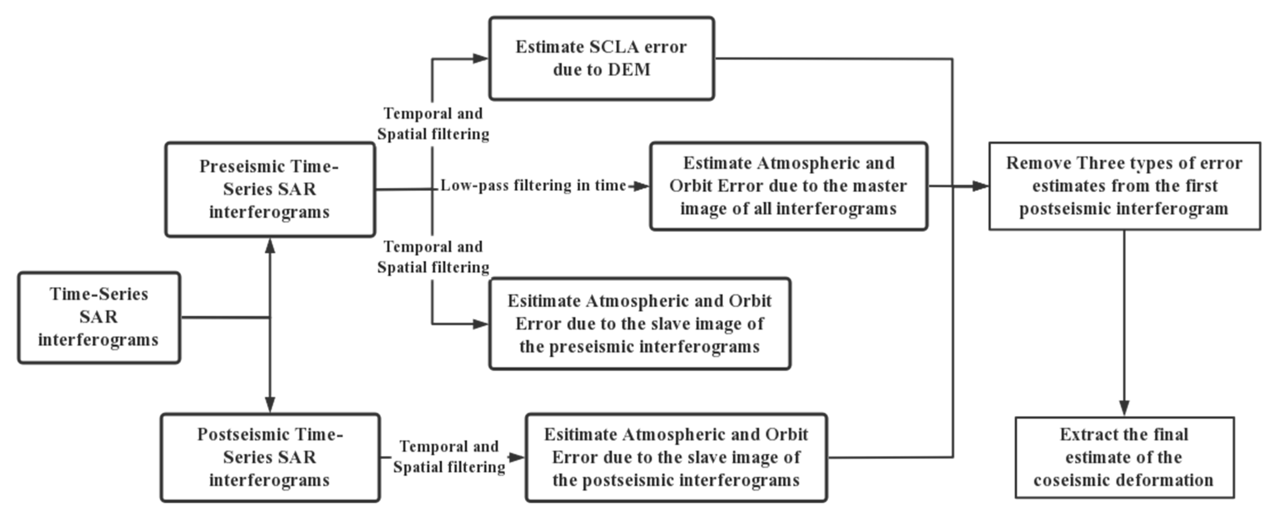
3.1. Time-Series InSAR Processing Method for Coseismic Deformation Field Extraction

In this study, we used a single master image interferometric configuration, specifically conventional PS-InSAR, and applied a spatio-temporal algorithm for phase unwrapping. Because the extracted deformation signals were abrupt, the main improvement of the method suggested in this study was the segmented time-series process for estimating various errors. The phase of the coseismic deformation contained in the post-seismic time-series interferogram can affect error estimates, resulting in incorrect estimates that affect the extraction of the final coseismic deformation signal. Therefore, this method devides unwrapped interferograms into pre-seismic and post-seismic sequences. To estimate the spatially correlated look angle (SCLA) error and the atmospheric and orbit error (AOE) due to the master image, we only used the pre-seismic time-series interferogram for spatio-temporal filtering. This prevented the phase of the coseismic deformation in the post-seismic interferograms from affecting the error estimation. Finally, AOE due to the slave images were separated from the interferogram by performing temporal filtering on the pre-seismic and post-seismic interferograms, respectively. In a general analysis, filtering was performed uniformly for all time-series interferograms and weak coseismic deformation signals may be erroneously filtered out as noise, which must be accounted for in any processing flow. The complete process flow is illustrated in Figure 2.

An SAR image acquired just before the earthquake was used as the master image, and co-registered with other pre-seismic and post-seismic images that were used as the slave images. The master and slave images were co-registered individually to perform differential interferometry. In this case, the coseismic deformation signal is not present in the pre-seismic interferogram but rather in the post-seismic interferogram. In StaMPS, the threshold is first set using the amplitude deviation method combined with phase stability estimates to select PS candidates, and then the wrapped phase is corrected to filter out spatially uncorrelated look angle errors. Finally, the phase of the PS candidates were unwrapped to recover the absolute deformation phase using the 3D spatio-temporal method. The phases in the unwrapped interferograms were divided into five terms:

$${\phi }_{\text{int}}={\phi }_D+{\phi }_A+{\phi }_O+{\phi }_{\theta }^c+{\phi }_n$$

(1)

where ${\phi }_{\mathrm{int}}$ indicates the unwrapped phase, ${\phi }_D$ indicates the surface deformation phase, ${\phi }_A$ indicates the error due to atmospheric effect, ${\phi }_O$ is the residual orbital error, ${\phi }_{\theta }^c$ is the residual phase due to the SCLA error, and ${\phi }_n$ is the term for noise due to other factors, for example, co-registration and phase unwrapping.

Because the pre-seismic and post-seismic time-series interferograms needed to be processed separately, two different expressions were used for the unwrapped phases before and after the earthquake. The spatially uncorrelated look angle errors were screened out before the interferogram was unwrapped, so that the remaining residual errors in the unwrapped interferometric phase of the digital elevation model (DEM) only included the SCLA errors. The other spatially correlated errors were divided into AOEs due to the master and slave images, where the AOEs due to the master image are present in each interferogram. The deformation phase and other error terms in the pre-seismic and post-seismic interferograms can be expressed by the following equations:

$${\phi }_{x,i}={\phi }_{D,x,i}^{non}+{\phi }_{\theta ,x,i}^c+{\phi }_{A,x,i}^s+{\phi }_{A,x,i}^m+{\phi }_{O,x,i}^s+{\phi }_{O,x,i}^m+{\phi }_{n,x,i}$$

(2)

$${\phi }_{x,j}={\phi }_{D,x,j}^{non}+{\phi }_{\cos \mathit{eismic},x,j}+{\phi }_{\theta ,x,j}^c+{\phi }_{A,x,j}^s+{\phi }_{A,x,j}^m+{\phi }_{O,x,j}^s+{\phi }_{O,x,j}^m+{\phi }_{n,x,j}$$

(3)

where $x$ denotes the master image, ${\phi }_{x,i}$ represents the unwrapped phase of the pre-seismic interferogram, ${\phi }_{x,j}$ represents the unwrapped phase of the post-seismic interferogram, and the superscripts m and s denote the contributions of the master and slave images to each spatially correlated error, respectively. ${\phi }_D^{non}$ denotes the surface deformation phase that does not include coseismic deformation signals and is present in all interferograms, and ${\phi }_{\cos eismic,x,j}$ represents the coseismic deformation phases included in the post-seismic interferogram.

When using a DEM for terrain phase estimation, DEM errors can lead to other terrain-related residual phases in the interferometric phase. DEM errors tend to be partially spatially correlated and mapped to look angle errors; therefore, the SCLA error accounts for most DEM errors [22]. An SCLA error is present in each pair of interferograms. Because the terrain undergoes substantial deformation after an earthquake, the post-seismic time-series interferograms containing the coseismic deformation signals were not involved in the estimation of the SCLA error in this study. The following equation represents the SCLA error due to the DEM:

$$\Delta {\phi }_{\theta }\approx \frac{4\pi }{\lambda }B\cos (\theta -\omega )\Delta \theta =\frac{4\pi }{\lambda }{B}_{\perp }\left(\theta \right)\Delta \theta$$

(4)

where $\lambda$ denotes the radar wavelength; $B$ denotes the baseline distance between the slave image and master image sensor position; $\theta$ denotes the look angle in the master image geometry; $\omega$ denotes the angle between the baseline and horizontal vectors; and $B_{\perp }\left(\theta \right)$ denotes the vertical component of the baseline.

Atmospheric conditions are unlikely to be identical when satellites make repeated observations of the ground; therefore, the path of the electromagnetic waves changes during propagation and produces phase delays during radar imaging, resulting in substantial errors in the measurement of surface deformation [23,24]. Both the positioning accuracy of the satellite orbit and atmospheric effects during operation can lead to biases when a satellite revisits the same position. Even with orbital parameters, it is not possible to completely remove orbital error streaks, and residual errors propagate with subsequent processing [25]. Especially in coseismic deformation measurements, orbital errors propagate into the interferometric phase and affect the final estimation of the deformation. The orbital and atmospheric errors are similar in their spatial and temporal properties; therefore, we adopted spatiotemporal filtering to separate the coseismic deformation signal from the AOEs. The AOE due to the master image in the interferometric phase was estimated first. Considering the effect of post-earthquake coseismic deformation on the estimation, only pre-seismic interferograms were selected to estimate this error. Low frequencies characterize the nonlinear deformation signal in both the time and space domains, whereas high frequencies characterize the AOE in the time domain [12]. Therefore, we performed low-pass filtering in the time dimension of the unwrapped phase for the pre-seismic interferogram to separate the surface deformation signal from the AOE due to the master image. The AOE due to the master image was removed from the interferogram, and an estimate of the master image AOE was obtained:

$${\Phi }^L\left\{{\phi }_{x,i}\right\}\approx {\phi }_{D,x,i}-\left({\phi }_{A,x,i}^m+{\phi }_{O,x,i}^m\right)$$

(5)

where ${\Phi }^L$ is the temporal low-pass filter operator.

To estimate the AOE due to slave images, separate spatio-temporal filtering was applyied to pre-seismic and post-seismic time-series interferograms. Given the high-frequency characteristics of the AOE in the time dimension, high-pass filtering was performed for the remaining phases in the pre-seismic and post-seismic time-series interferograms. While the AOE has low-frequency characteristics in the spatial dimension, the high-pass filter allows spatial low-pass filtering for the signal output, and the spatial filter outputs the final estimate of the AOE due to the slave image:

$${\Psi }^L\left\{{\Phi }^H\left\{{\phi }_{x,i}\right\}\right\}\approx {\phi }_{A,x,i}^s+{\phi }_{O,x,i}^s+{\phi }_{n,x,i}$$

(6)

$${\Psi }^L\left\{{\Phi }^H\left\{{\phi }_{x,j}\right\}\right\}\approx {\phi }_{A,x,j}^s+{\phi }_{O,x,j}^s+{\phi }_{n,x,j}$$

(7)

where ${\Phi }^H$ is the temporal high-pass filtering operator and ${\Psi }^L$ is the spatial low-pass filtering operator.

The phase of the interferogram formed by the SAR images on the nearest date before and after the earthquake date contains the most accurate coseismic deformation signal; therefore, the final coseismic deformation estimate is only based on the interferometric phase in this interferogram. The DEM-induced SCLA error, AOE due to the master image, and estimated AOE due to the slave image were first removed from the interferometric phase, and other elevation-related errors were then removed from the remaining phases. Finally, the extracted coseismic deformation phases were spatially filtered to remove other spatial noises and obtain a final coseismic deformation phase estimate with high precision. The coseismic deformation estimate was given by the following equation:

$$\begin{array}{ll}{\phi }_{\text{cos} \mathit{\text{eismic}}}& \approx {\phi }_{x,x+1}-{\phi }_{\theta ,x,x+1}^c-({\phi }_{A,x,x+1}^S+{\phi }_{O,x,x+1}^S)-({\phi }_{A,x,x+1}^m+{\phi }_{O,x,x+1}^m)\\ & \approx {\phi }_{\text{cos} \mathit{\text{eismic}},x,x+1}\end{array}$$

(8)

where $x+1$ indicates the first post-seismic image to the date of the earthquake. As other surface deformation ${\phi }_{D,x,x+1}^{non}$ is negligible, ${\phi }_{\cos eismic}$ represents the final estimate of coseismic deformation.

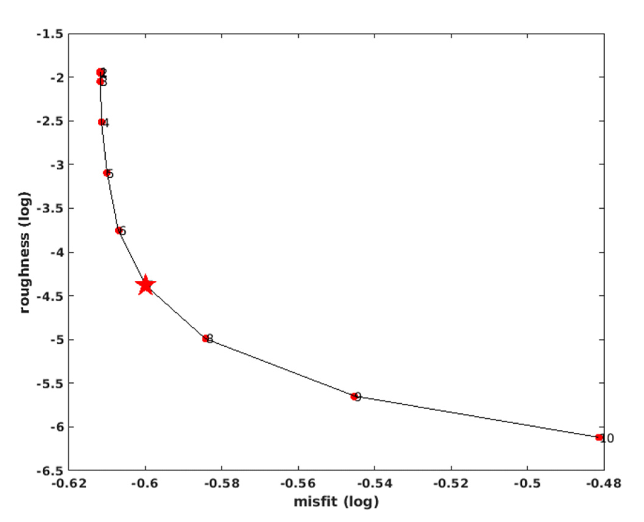
3.2. Inversion of Fault Geometry Parameters and Slip Distribution

Taking the coseismic deformation fields extracted by the above time-series InSAR processing method as constraints, we performed an inversion of the 2021 Yangbi M_W 6.1 earthquake to obtain the fault geometry parameters and fault slip distribution. Based on this, we studied the fault activity and rupture characteristics of this earthquake in detail. In this study, we used the Geodetic Bayesian Inversion Software (GBIS) developed by Bagnardi and Hooper in 2018 to perform nonlinear homogeneous and slip inversion of the best fault geometry parameters for this earthquake [26]. GBIS uses a Bayesian probabilistic inversion algorithm for InSAR observations derived from the original datasets. In the Bayesian framework, an optimal set of source model parameters is extracted from the posterior probability density function (PDF) by quickly estimating the best model parameters and associated uncertainties through efficient sampling the posterior PDF. In the process of seismic inversion using this method, the Markov chain Monte Carlo (MCMC) method was used to perform sampling [27], which was controlled in combination with the Metropolis Hastings algorithm [28,29]. Automatic step-size selection can control the random walk step of each model parameter to ensure sampling efficiency. After multiple iterations, the set of model parameters with the maximum a posterior probability after pre-assigned iterations was selected.

We inverted the fault based on the elastic half-space dislocation model proposed by Okada in 1985, which provides the relationship between the surface deformation and fault slip at depth [30]. This elastic dislocation model provides nine source model parameters, including the length, width, depth, X and Y coordinates of the lower edge midpoint, dip and strike of the fault, and dip slip and strike slip. First, the seismic region was modeled as a uniform rectangular fault plane and the geometric parameters of the fault were accurately estimated using the GBIS algorithm. To obtain the dislocation distribution across a fault, it is necessary to invert the slip distribution across the fault plane. Because the slip distribution is nonuniform, the inversion of the fault slip distribution is equivalent to solving the optimal value of a linear problem. Based on the parameters of the fault geometric model, the fault plane was discretized into several uniform sub-fault planes, and the slip distribution of each sub-fault plane was then inverted to further obtain the fine slip distribution of the entire fault. The slip parameter model coefficient matrix is called Green’s function matrix, and we chose the constrained least-squares algorithm to estimate slip distribution [31]. As Green’s function matrix is severely rank deficient, the Laplace smoothing matrix was added to the inversion for regularization, and the L-curve method was used to select the best regularization parameters [32].

4. Results

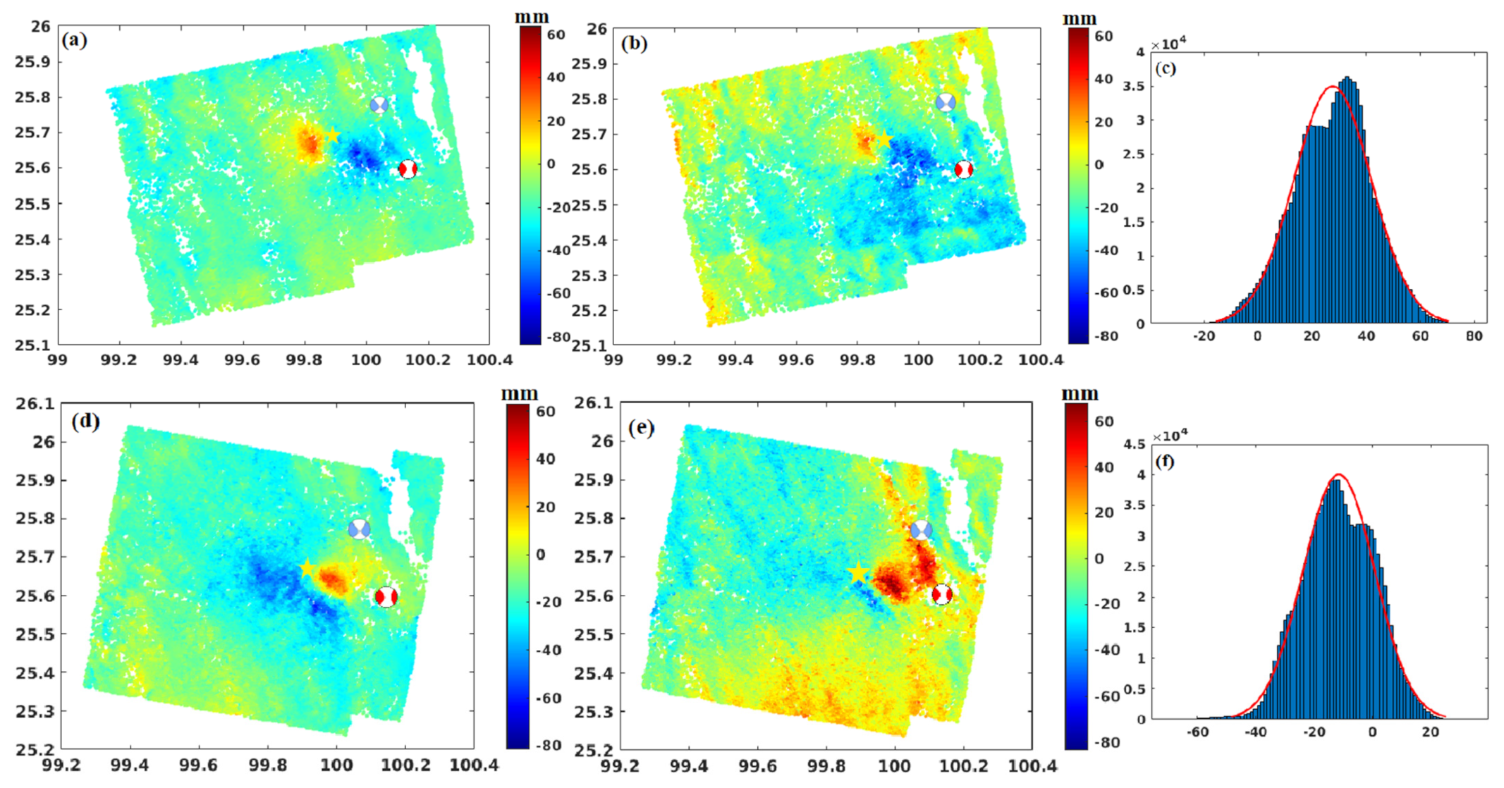
4.1. InSAR Coseismic Deformation Field

In this study, the time-series InSAR processing method was applied to the Yangbi M_W 6.1 earthquake using ESA Sentinel-1 A satellite Single Look Complex (SLC) images as the data source. We acquired 36 SLC images from ascending track AT99 and 34 SLC images from descending track DT135, with an image date interval of 12 days, consistent with the satellite revisit cycle. For the Yangbi M_W 6.1 earthquake occurred on 21 May 2021, the date for the selected master image in the ascending track data is 20 May 2021 and the date of the selected master image in the descending track data is 10 May 2021. Co-registration and differential interferometry were performed using the Swiss interferometry software GAMMA [33], and the corresponding precise orbit ephemerides were used to provide orbit information. ALOS World 3D-30 m DEM data was selected as an external reference DEM to assist SAR image co-registration and topographic phase removal in differential interferometry. We chose the built-in algorithm of StaMPS to perform PS point selection and phase decoupling for all interferograms and then used the time-series processing method adopted in this study to accurately estimate each error. Finally, we extracted the coseismic deformation phases of the Yangbi M_W 6.1 earthquake in the ascending and descending tracks, and obtained the coseismic deformation displacement in the LOS direction after conversion.

It can be seen from the interferograms in Figure 3 that the long axis of the main deformation field of the Yangbi earthquake is roughly in the NW direction, and it can be assumed that the seismic traces divide the deformation area into eastern and western plates, showing an asymmetric distribution. The range of the coseismic deformation field in the ascending track was approximately 22 km in the north–south direction and approximately 24 km in the east–west direction. The maximum LOS displacement was approximately −74 mm in the east plate and 44 mm in the west plate. The range of the descending coseismic deformation field was approximately 22 km in the north–south direction and approximately 20 km in the east–west direction, and the maximum LOS displacement was approximately 43 mm in the east plate and −62 mm in the west plate. A positive value of LOS displacement indicates that the surface deformation is moving towards the satellite, whereas a negative value indicates that the deformation is moving away from the satellite. Differences in the satellite side view and flight attitude in the ascending and descending tracks results in different imaging patterns. Consequently, the coseismic deformations obtained from the ascending and descending tracks differ in their spatial distribution and magnitude. Based on the above results, the observed values of deformation in the east and west plates extracted from the ascending and descending tracks showed exactly opposite trends. Therefore, this earthquake had characteristics consistent with strike-slip type fault deformation. Because the coseismic deformation area extends along the NW–SE direction, it can be tentatively concluded that the Yangbi earthquake caused a rupture along the NW–SE direction. Moreover, there was no obvious decoherence area caused by surface rupture in the deformation area of either track, so the earthquake rupture did not reach the surface.

In this study, we compared the coseismic deformation extracted by time-series InSAR method with that extracted by D-InSAR. The two different coseismic deformations are shown in Figure 4. Figure 4a,d show the LOS coseismic deformation in the ascending and descending tracks after the elimination of each error using time-series InSAR processing, respectively. Figure 4b,e show the LOS coseismic deformations in the ascending and descending tracks extracted from the single differential interferogram without error removal, respectively. Figure 5a,d show the SCLA error values estimated by the time-series analysis, Figure 5b,e show the estimated AOE due to the master image, and Figure 5c,f show the estimated AOE due to the slave images. For the ascending track, the eastern plate of the deformation field without error removal is mainly masked by the master AOE, and the western plate is mainly affected by the SCLA error and the slave AOE. For the descending track, the eastern plate of deformation field without error removal is mainly affected by the master AOE and the SCLA error, and the western plate is affected by the slave AOE. To demonstrate the effectiveness of the above time-series InSAR processing methods in removing errors, we also performed a quantitative analysis of the coseismic deformations extracted by the two different methods. We calculated the differences between the coseismic deformation displacements extracted by the time-series InSAR and the coseismic deformations extracted from the single interferogram without removing the errors. Figure 4c,f show histograms of the frequency distribution of the difference between the two deformations in the ascending and descending tracks, respectively. The difference between the two different coseismic deformations in the ascending track ranges from −20 mm to 70 mm, and the RMS of the difference is 31.05 mm. The difference between the two different coseismic deformations in the descending track ranges from −60 mm to 20 mm, and the RMS of the difference is 16.87 mm. After analysis, we concluded that the time-series InSAR processing method used in this study has a significant effect in estimating errors, which makes the extracted coseismic deformation field more accurate and clarifies the deformation field.

4.2. Fault Geometry Parameters

Before fault inversion, it is necessary to down-sample the coseismic deformation data to reduce the redundancy caused by the large number of data points and reduce the computational cost of inversion. In this study, we chose an adaptive quadtree algorithm to down-sample the ascending and descending LOS deformation data of the Yangbi M_W 6.1 earthquake, and maintained the dense deformation points in the near deformation field [34,35,36]. The down-sampled data points retained better deformation field characteristics and improved the subsequent calculation efficiency. With the ascending and descending down-sampled deformation points as common constraints, we used the GBIS to invert the fault geometry parameters of the Yangbi Mw 6.1 earthquake. In the framework of the GBIS algorithm, the MCMC method was used to sample the deformation data, and after 10⁶ iterations, the burn-in period of the first 2 × 10⁴ iterations was removed to determine the optimal set of model parameters.

Based on the Okada elastic half-space dislocation model, we used the GBIS algorithm to obtain the nine source parameters of the Yangbi earthquake, which are listed in

Table 2. Seismic fault geometric parameters of the 2021 Yangbi M_W 6.1 earthquake.

Parameter	Optimal	Mean	Median	2.50%	97.50%
Length (m)	17,233.9	17,295.8	17,275.5	15,465.8	19,263.9
Width (m)	1032.87	1332.03	1023.97	606.288	4089.61
Depth (m)	5498.51	5362.01	5411.48	4384.8	5931.69
Dip (°)	76.9801	78.2016	77.7524	83.8792	75.131
Strike (°)	133.428	133.559	133.544	130.624	136.601
X center (m)	9031.41	8813.28	8828.41	9525.23	8018.04
Y center (m)	10,176.4	10,319.8	10,264.8	10,928.8	10,011.5
Strike slip (m)	2.56309	2.48903	2.55033	0.685637	3.91905
Dip slip (m)	0.133527	0.123478	0.112916	0.0114473	0.287731

, including the final maximum a posteriori probability solution and a 95% confidence interval. Here, 2.50% and 97.50% represent the upper and lower limits of the confidence intervals, respectively. There was little difference between the different parameters obtained from the inversion, proving the reliability of the inversion results. According to the optimal solution, the fault length of the Yangbi M_W 6.1 earthquake was approximately 17 km and the fault width was approximately 1033 m. The dip and strike of the fault were 76.98° and 313.43°, respectively, which are close to the values provided by the GCMT. The optimal solution of the X and Y coordinates at the midpoint of the lower edge is converted to a geographic coordinate system of 25.6441° N and 99.9261° E, corresponding to a depth of approximately 5.8 km. After inversion, we also obtained the slip components in the dip and strike directions, where the strike-slip component was 2.56 m and the dip-slip component was 0.13 m. Therefore, we can conclude that the slip direction of the fault mechanism is consistent with a large right-lateral strike-slip component and a small thrust component. In conclusion, the optimal fault geometric parameters obtained by GBIS inversion are in agreement with the focal mechanism solutions provided by the USGS and GCMT.

4.3. Fault Slip Distribution

In this study, a constrained least-squares algorithm was used to invert the fault slip distribution. First, the fault geometry parameters calculated by GBIS were introduced into the linear inversion model, Green’s function coefficient matrix was solved, and a Laplace smoothing matrix was used to constrain the slip roughness. According to the GBIS fault geometry parameters, the strike of the fault model was fixed at 133.43°, and the dip angle was fixed at 76.98°. The fault activity mode was right-lateral strike-slip; therefore, the range of the rake was set to 90°–180°. The fault plane extended to 30 km along the strike, and to 15 km along the dip. This fault plane was divided into 20 × 15 sub-fault planes to analyze the fine slip distribution. The optimal slip factor was determined by plotting the L-curve between the roughness and misfit of the slip distribution, which assessed the reasonableness of the inversion results and obtained the optimal fault slip distribution. Figure 6 shows the roughness and relative misfit corresponding to the optimal smoothing factor determined from the L curve.

Figure 7 shows the fault-slip distribution determined by inversion. The direction of the arrow indicates the movement direction of each sub-fault plane, indicating that the slip direction of the entire fault plane is correct. Figure 7 illustrates that there is a main fracture area in the Yangbi earthquake, concentrated at 6–24 km along the strike direction and 3–12 km down the dip direction. It was also determined that the rupture caused by the earthquake did not reach the surface. The 3D slip distribution indicated that the slip-concentrated area is located at a depth of 5–10 km, and the maximum slip was approximately 0.6738 m, occurring at a depth of 5.5 km. Combined with the geometric parameters of the fault and the results of slip distribution, it can be determined that the fault mechanism of Yangbi earthquake is dominated by a right-lateral component. Assuming that the shear modulus is 30 GPa, the inversion results show that the seismic moment energy released by this earthquake is approximately 1.58 × 10¹⁸ N∙ m, and the corresponding moment magnitude is approximately M_W 6.07, which is slightly lower than the moment magnitude of M_W 6.1 provided by the USGS and GCMT. Finally, it was determined that the epicenter of the Yangbi earthquake is located at 25.6388° N and 99.9175° E, which is close to the focal center provided by the USGS.

To evaluate the reliability of the inversion results, we simulated the LOS coseismic deformation fields in the ascending and descending tracks according to the inversion results of the fault slip distribution. After obtaining models of the coseismic deformation fields for the ascending and descending tracks, we calculated the residuals by subtracting them from the deformation observations obtained using the time-series InSAR method and then judged the reliability of the fault inversion based on the magnitude of the residuals. We also performed an inversion of the fault geometry and slip distribution on the coseismic deformation data extracted by a single interferogram to demonstrate that the coseismic deformation extracted by the time-series InSAR method is more accurate than that extracted by D-InSAR. The fault models were then fitted based on the results of the slip distribution inversion, and the fitting residuals between the InSAR observations and the models were calculated.

As shown in Figure 7c, many errors remained in the deformation results extracted using only a single interferogram, and the slip distribution inversion based on this dataset was largely disturbed, and as a result the slip distribution model to explain the data well. Figure 8 shows the observation values of the ascending and descending down-sampled LOS coseismic deformation fields extracted by the two different methods, the model values fitted according to slip distribution inversion, and the residuals between them. Comparing the inversion results of the two different datasets, it can be seen from Figure 8c,f that the LOS deformation field model simulated by the deformation dataset extracted by time-series InSAR is highly consistent with the observation values, and the fitting residual values for ascending and descending tracks are both less than 0.02 m, indicating the high fitting degree between the model and observation values and proving the reliability of the inversion results. As shown in Figure 9a,b, the residuals between the observed LOS deformation in the ascending track extracted by the time-series InSAR method and the model values fitted by the inversion range of −0.03~0.03 m with a residual RMS of 0.79 cm, while the residuals between the observed LOS deformation in the descending track and the model values fitted by inversion range from −0.05~0.03 m with a residual RMS of 0.91 cm. Figure 8i,l show that the fitting residuals between the LOS coseismic deformation fitted model value according to the deformation dataset extracted by D-InSAR and the observation value are large, and the fitting degree is relatively low because the error in the observation data affected the simulation of the model for real data. As shown in Figure 9c,d the residuals between the observed ascending LOS deformation extracted by D-InSAR and the model values fitted by inversion range from −0.04 m to 0.04 m with a residual RMS of 1.34 cm, while the residuals between the observed ascending LOS deformation and the model values fitted by inversion range from −0.05 m to 0.05 m with a residual RMS of 1.32 cm. Therefore, the errors in the deformation data observed by InSAR have a negative impact on seismic inversion, and the comparison proves the effectiveness of the time-series InSAR method used in this study to extract the coseismic deformation.

5. Discussion

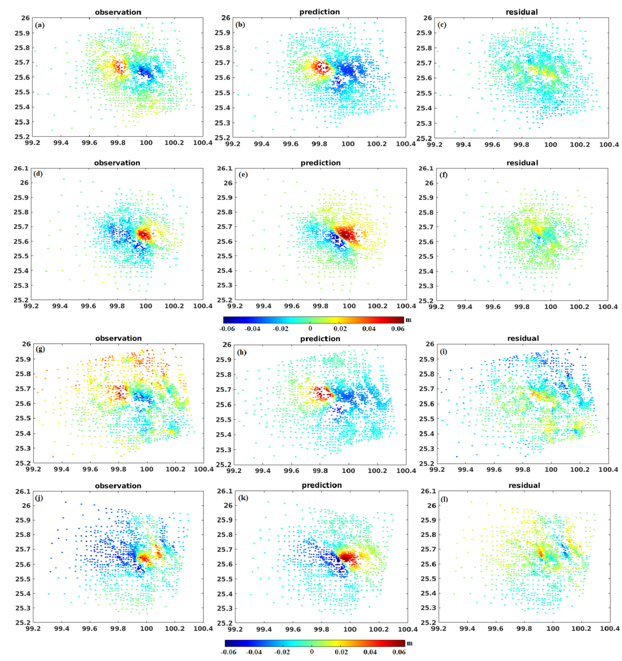
5.1. Validation of Methods Using Synthetic Data

To verify the effectiveness of the time-series InSAR processing method used in this paper to eliminate errors and extract coseismic deformations, synthetic time-series interferograms based on the inversion-fitted LOS coseismic deformations in the descending track. The inverse model of the downsampled LOS coseismic deformation was used as the true coseismic deformation of the synthetic data. Because the model values are the down-sampled data, we used an interpolation algorithm to obtain interferograms corresponding to the original data size. First, all deformation phases of the pre-seismic interferograms were set to 0, and all deformation phases of post-seismic interferograms were set to the true deformation phases. Then, we added errors estimated using the time-series analysis as noise to the corresponding interferogram, such that the interferometric phase of the synthesized time-series interferograms were closer to the actual characteristics of the unwrapped interferogram. Finally, we used the time-series InSAR processing method to perform a time-series analysis of the synthesized time-series unwrapped interferograms to estimate errors, and obtained estimates of the LOS coseismic deformation after removing the errors.

Figure 10a shows the interpolated downgraded LOS coseismic deformation model values as the true coseismic deformation, Figure 10b shows the coseismic deformation extracted from the first synthesized post-seismic interferogram, and Figure 10c shows the coseismic deformation extracted from the synthesized time-series interferogram with time-series InSAR processing. It is evident from Figure 10 that the difference between the deformation field including noise and the real deformation simulation is large, and the RMS of the difference between the two is 16.68 mm. However, the deformation extracted by the time-series analysis was similar to the real deformation field pattern. Figure 10e shows the frequency distribution of the difference between the deformation extracted by the time-series processing and the real deformation, and here the difference is no greater than 1 cm and the RMS of the difference is reduced to 8.77 mm, with a very small difference of no more than 1 cm. After validation using the synthetic dataset, it was demonstrated that it is feasible and effective to use the time-series InSAR processing method for error estimation using time-series interferograms and to extract the coseismic deformation. We concluded that the use of time-series analysis can improve estimate the errors in the unwrapped interferograms and as well as the extraction accuracy of the coseismic deformation.

5.2. Advantages of Time-Series InSAR Processing Method for Coseismic Deformation Extraction

A major contribution of this study is the use of a specifically designed time-series InSAR technique to extract the coseismic deformation information. A time-series analysis can eliminate disturbance that cannot be resolved using conventional D-InSAR techniques. The errors due to atmospheric delay and the deformation phase both have low-frequency spatial characteristics. It is difficult to distinguish these to eliminate atmospheric effects by using a single interferogram. The D-InSAR technique uses orbital parameters to eliminate orbital errors in the interferogram. However, the residual phase ramp has a significant impact on the final measurement results. The time-series approach used in this study can estimate three disturbance terms: terrain-related residual errors, errors owing to atmospheric delays, and orbital errors. The application of this approach to the Yangbi M_W 6.1 earthquake proves that the time-series InSAR processing technique can accurately resolve certain unavoidable problems associated with the D-InSAR technique. The coseismic deformation phases contained in the post-seismic time-series interferograms have a significant impact on the error estimates, resulting in incorrect results. Only pre-seismic time-series interferograms are used to estimate the SCLA error and the master AOE, which prevents the coseismic deformation of the post-seismic interferograms from influencing the estimation errors. By performing temporal filtering on the pre-seismic and post-seismic interferograms separately, the slave AOE can be accurately separated from the interferograms. Moreover, the coseismic deformations of moderate earthquakes are not as obvious as those of large magnitude earthquakes, and often the various errors in the differential interferograms can often mask the true deformations, resulting in the poor accuracy of the extracted deformations. The time-series InSAR processing method can retrieve weak coseismic signals by eliminating various errors and avoids the leakage of coseismic deformation signals into error components. Compared to the deformation field extracted by D-InSAR, the coseismic deformation extracted by the processing method in this study shows better agreement with the actual pattern of earthquake deformation. By investigating the inversion results, we found that the errors remaining in the D-InSAR results had a significantly negative impact on the inversion. The time-series InSAR proessing method used in this study is based on PS-InSAR technology; therefore, the time-series information of all persistent scatterers can be retained to observe the pre-seismic and post-seismic deformation trends.

6. Conclusions

With the sentinel-1 SAR images, we used a time-series InSAR method to extract the coseismic deformation field. The geometric parameters and slip distribution of the fault were then inverted with the down-sampled deformation datasets as a constraint. The following conclusions were drawn.

(1) The time-series InSAR method can estimate the erroneous terms accurately, including the DEM error and the AOE due to master image and slave images. Analysis of both synthetic and real-world datasets validated the effectiveness of this processing method.

(2) The deformation fields extracted by the time-series InSAR method displayed opposite trends in ascending and descending tracks. In the ascending LOS direction, the maximum displacement of the eastern disk was approximately -74 mm and that of the western disk is approximately 44 mm. In the descending LOS direction, the maximum displacement of the eastern disk was approximately 43 mm, and that of the western disk is approximately −62 mm.

(3) The fault inversion results showed that the strike of the seismic fault was 133.43°, the dip was 76.98°, and the maximum slip was 0.6738 m, located at a depth of 5.5 km. The earthquake was a right-lateral strike-slip event with a moment magnitude (M_W) of 6.07; this finding is close to the source mechanisms proposed by the USGS and GCMT.

References

1. Massonnet, D.; Rossi, M.; Carmona, C.; Adragna, F.; Peltzer, G.; Feigl, K.; Rabaute, T. The displacement field of the Landers earthquake mapped by radar interferometry. Nature 1993, 364, 138–142. [Google Scholar] [CrossRef]
2. Fialko, Y.; Sandwell, D.; Simons, M.; Rosen, P. Three-dimensional deformation caused by the Bam, Iran, earthquake and the origin of shallow slip deficit. Nature 2005, 435, 295–299. [Google Scholar] [CrossRef]
3. Peltzer, G.; Rosen, P. Surface Displacement of the 17 May 1993 Eureka Valley, California, Earthquake Observed by SAR Interferometry. Science 1995, 268, 1333–1336. [Google Scholar] [CrossRef]
4. Ferretti, A.; Prati, C.; Rocca, F. Nonlinear subsidence rate estimation using permanent scatterers in differential SAR interferometry. IEEE Trans. Geosci. Remote Sens. 2000, 38, 2202–2212. [Google Scholar] [CrossRef] [Green Version]
5. Rogers, A.; Ingalls, R.P. Venus: Mapping the Surface Reflectivity by Radar Interferometry. Science 1969, 165, 797–799. [Google Scholar] [CrossRef]
6. Lundgren, P.; Usai, S.; Sansosti, E.; Lanari, R.; Tesauro, M.; Fornaro, G.; Berardino, P. Modeling surface deformation observed with synthetic aperture radar interferometry at Campi Flegrei caldera. J. Geophys. Res. Solid Earth 2001, 106, 19355–19366. [Google Scholar] [CrossRef] [Green Version]
7. Ferretti, A.; Prati, C.; Rocca, F. Permanent scatterers in SAR interferometry. IEEE Trans. Geosci. Remote Sens. 2001, 39, 8–20. [Google Scholar] [CrossRef]
8. Colesanti, C.; Ferretti, A.; Novali, F.; Prati, C. SAR monitoring of progressive and seasonal ground deformation using the permanent scatterers technique. IEEE Trans. Geosci. Remote Sens. 2003, 41, 1685–1701. [Google Scholar] [CrossRef] [Green Version]
9. Ferretti, A.; Prati, C.; Rocca, F. Permanent scatterers in SAR interferometry. In Proceedings of the IEEE 1999 International Geoscience and Remote Sensing Symposium, IGARSS’99 (Cat. No. 99CH36293). Hamburg, Germany, 28 June–2 July 1999; pp. 1528–1530. [Google Scholar]
10. Ferretti, A.; Savio, G.; Barzaghi, R.; Borghi, A.; Rocca, F. Submillimeter Accuracy of InSAR Time Series: Experimental Validation. IEEE Trans. Geosci. Remote Sens. 2007, 45, 1142–1153. [Google Scholar] [CrossRef]
11. Hooper, A.; Zebker, H.; Segall, P.; Kampes, B. A new method for measuring deformation on volcanoes and other natural terrains using InSAR persistent scatterers. Geophys. Res. Lett. 2004, 31. [Google Scholar] [CrossRef]
12. Hooper, A.; Segall, P.; Zebker, H. Persistent scatterer interferometric synthetic aperture radar for crustal deformation analysis, with application to Volcán Alcedo, Galápagos. J. Geophys. Res. Solid Earth 2007, 112. [Google Scholar] [CrossRef] [Green Version]
13. Zhang, L.; Hu, J.; Ding, X.; Wen, Y.; Liang, H. Estimation of Coseismic Deformation with Multitemporal Radar Interferometry. IEEE Geosci. Remote Sens. Lett. 2021, 19, 1–5. [Google Scholar] [CrossRef]
14. Luo, H.; Wang, T.; Wei, S.; Liao, M.; Gong, J. Deriving centimeter-level coseismic deformation and fault geometries of small-to-moderate earthquakes from time-series Sentinel-1 SAR images. Front. Earth Sci. 2021, 9, 32. [Google Scholar] [CrossRef]
15. Zhang, K.; Gan, W.; Liang, S.; Xiao, G.; Dai, C.; Wang, Y.; Li, Z.; Zhang, L.; Ma, G. Coseismic displacement and slip distribution of the 2021 May 21. MS 6.4, Yangbi Earthquake derived from GNSS observations. Chin. J. Geophys. 2021, 64, 2253–2266. [Google Scholar]
16. Zhang, B.; Xu, G.; Lu, Z.; He, Y.; Peng, M.; Feng, X. Coseismic Deformation Mechanisms of the 2021 Ms 6.4 Yangbi Earthquake, Yunnan Province, Using InSAR Observations. Remote Sens. 2021, 13, 3961. [Google Scholar] [CrossRef]
17. Xu, X.; Ding, Z.; Shi, D.; Li, X. Receiver function analysis of crustal structure beneath the eastern Tibetan plateau. J. Asian Earth Sci. 2013, 73, 121–127. [Google Scholar] [CrossRef]
18. Tapponnier, P.; Xu, Z.; Roger, F.; Meyer, B.; Arnaud, N.; Wittlinger, G.; Yang, J. Oblique Stepwise Rise and Growth of the Tibet Plateau. Science 2001, 294, 1671–1678. [Google Scholar] [CrossRef]
19. Su, Y.J.; Qin, J.Z. Strong Earthquake Activity and Relation to Regional Neotectonic Movement in Sichuan-Yunnan Region. Earthq. Res. China 2001, 17, 24–34. [Google Scholar]
20. Wang, E. The Jinsha River transform fault sedimentary basin. Sci. Geol. Sin. 1985, 33–42. [Google Scholar]
21. Allen, C.R.; Gillespie, A.R.; Han, Y.; Sieh, K.E.; Zhang, B.; Zhu, C. Red River and associated faults, Yunnan Province, China: Quaternary geology, slip rates, and seismic hazard. Geol. Soc. Am. Bull. 1984, 95, 686–700. [Google Scholar] [CrossRef]
22. Hooper, A.J. Persistent Scatter Radar Interferometry for Crustal Deformation Studies and Modeling of Volcanic Deformation. Ph.D. Dissertation, Stanford University, Stanford, CA, USA, 2006. [Google Scholar]
23. Ding, X.-L.; Li, Z.-W.; Zhu, J.-J.; Feng, G.-C.; Long, J.-P. Atmospheric effects on InSAR measurements and their mitigation. Sensors 2008, 8, 5426–5448. [Google Scholar] [CrossRef] [Green Version]
24. Emardson, T.; Simons, M.; Webb, F. Neutral atmospheric delay in interferometric synthetic aperture radar applications: Statistical description and mitigation. J. Geophys. Res. Solid Earth 2003, 108. [Google Scholar] [CrossRef]
25. Fialko, Y. Interseismic strain accumulation and the earthquake potential on the southern San Andreas fault system. Nature 2006, 441, 968–971. [Google Scholar] [CrossRef]
26. Bagnardi, M.; Hooper, A. Inversion of surface deformation data for rapid estimates of source parameters and uncertainties: A Bayesian approach. Geochem. Geophys. Geosyst. 2018, 19, 2194–2211. [Google Scholar] [CrossRef]
27. Mosegaard, K.; Tarantola, A. Monte Carlo sampling of solutions to inverse problems. J. Geophys. Res. 1995, 100, 12431–12447. [Google Scholar] [CrossRef]
28. Metropolis, N.; Rosenbluth, A.W.; Rosenbluth, M.N.; Teller, A.H.; Teller, E. Equation of State Calculations by Fast Computing Machines. J. Chem. Phys. 1953, 21, 1087–1092. [Google Scholar] [CrossRef] [Green Version]
29. Hastings, W.K. Monte Carlo sampling methods using Markov chains and their applications. Biometrika 1970, 57, 97–109. [Google Scholar] [CrossRef]
30. Okada, Y. Surface deformation due to shear and tensile faults in a half-space. Bull. Seismol. Soc. Am. 1985, 75, 1135–1154. [Google Scholar] [CrossRef]
31. Wang, C.; Wang, X.; Xiu, W.; Zhang, B.; Liu, P. Characteristics of the Seismogenic Faults in the 2018 Lombok, Indonesia, Earthquake Sequence as Revealed by Inversion of InSAR Measurements. Seismol. Res. Lett. 2020, 91, 733–744. [Google Scholar] [CrossRef]
32. O’Leary, D.; Hansen, P.C. The Use of the L-Curve in the Regularization of Discrete Ill-Posed Problems. SIAM J. Sci. Comput. 1993, 14, 1487–1503. [Google Scholar]
33. Wegmüller, U.; Werner, C. Gamma SAR processor and interferometry software. In Proceedings of the 3rd ERS Scientific Symposium, Florence, Italy, 17–20 March 1997; pp. 1687–1692. [Google Scholar]
34. Jónsson, S.; Zebker, H.; Segall, P.; Amelung, F. Fault slip distribution of the 1999 M w 7.1 Hector Mine, California, earthquake, estimated from satellite radar and GPS measurements. Bull. Seismol. Soc. Am. 2002, 92, 1377–1389. [Google Scholar] [CrossRef]
35. Simons, M.; Fialko, Y.; Rivera, L. Coseismic deformation from the 1999 M w 7.1 Hector Mine, California, earthquake as inferred from InSAR and GPS observations. Bull. Seismol. Soc. Am. 2002, 92, 1390–1402. [Google Scholar] [CrossRef]
36. Decriem, J.; Árnadóttir, T.; Hooper, A.; Geirsson, H.; Sigmundsson, F.; Keiding, M.; Ófeigsson, B.; Hreinsdóttir, S.; Einarsson, P.; Lafemina, P.; et al. The 2008 May 29 earthquake doublet in SW Iceland. Geophys. J. Int. 2010, 181, 1128–1146. [Google Scholar] [CrossRef] [Green Version]
Figure 1. Regional tectonic background of Yangbi and the surrounding areas. The red and blue beach balls represent the focal mechanisms of the 2021 Yangbi MW 6.1 earthquake provided by the Global Centroid Moment Tensor (GCMT) and the United States Geological Survey (USGS), respectively; the gray lines denote the major active faults in this area; the yellow star is the epicenter provided by the China Earthquake Networks Center (CENC); the green dots and the purple dots indicate foreshocks and aftershocks, respectively.
Remotesensing 14 01017 g001
Figure 2. Time-series InSAR processing flow for coseismic deformation extraction.
Remotesensing 14 01017 g002
Figure 3. Ascending and descending interferograms of the 2021 Yangbi MW 6.1 earthquake: (a) interferogram in the ascending track; (b) interferogram in the descending track.
Remotesensing 14 01017 g003
Figure 4. LOS coseismic deformation displacement: (a,d) represent the LOS coseismic deformation displacements in the ascending and descending tracks extracted by time–series InSAR, respectively; (b,e) represent the LOS coseismic deformation displacements in the ascending and descending tracks extracted by D–InSAR, respectively; and (c,f) represent the frequency distribution histograms of the LOS deformation differences in the ascending and descending tracks, respectively.
Remotesensing 14 01017 g004
Figure 5. Error diagrams: (ac) represent the SCLA error, master AOE, and slave AOE estimated from the ascending data, respectively; and (df) represent the SCLA error, master AOE, and slave AOE estimated from the descending data, respectively.
Remotesensing 14 01017 g005
Figure 6. Trade–off curve between the misfit and model roughness. The star indicates optimal smoothing factor.
Remotesensing 14 01017 g006
Figure 7. Different fault slip distribution models from two InSAR deformation datasets: (a,b) are two–dimensional (2D) and three–dimensional (3D) displays of fault slip distribution inverted based on deformation results extracted by time–series InSAR, respectively; (c,d) are 2D and 3D displays of fault slip distribution based on deformation results extracted from a single interferogram, respectively; the arrow indicates the movement direction of each sub–fault plane.
Remotesensing 14 01017 g007
Figure 8. LOS coseismic deformation model fitting results based on the time-series InSAR and D–InSAR deformation datasets: (ac) represent ascending LOS deformation observations, predicted model values, and residuals, respectively; all are based on time–series InSAR data; (df) represent descending LOS deformation observations, model values, and residuals, respectively, based on time-series InSAR data; (gi) represent ascending LOS deformation observations, model values, and residuals, respectively, based on D–InSAR data; and (jl) represent descending LOS deformation observations, model values, and residuals, respectively, based on D–InSAR data.
Remotesensing 14 01017 g008
Figure 9. Histograms of residual frequency distributions: (a,b) indicate the ascending and descending residual distributions between the time–series InSAR–based deformation and its inversion–fitted model values, respectively; and (c,d) indicate the ascending and descending residual distributions between the D–InSAR–extracted deformation and its inversion-fitted model values, respectively.
Remotesensing 14 01017 g009
Figure 10. (a) represents the true coseismic deformation of the synthetic dataset; (b) represents the coseismic deformation extracted from the unwrapped interferogram after adding noise; (c) represents the coseismic deformation extracted from the synthetic dataset by the time–series InSAR processing method; (d) is the histogram of the difference distribution between the deformation after adding noise and the true deformation; and (e) is the histogram of the difference distribution between the deformation extracted by the time–series processing and the true deformation.
Remotesensing 14 01017 g010