1. Introduction
Gas flaring sites (GFs) have a strong impact on Earth’s system [
1,
2,
3], since they represent an important source of greenhouse gas (GHG) emission [
4,
5,
6].
Controlling anthropogenic GHGs is important to mitigate global warming for human sustainable development [
7]. Therefore, an accurate investigation of GFs is critical to evaluate the effects of emission reduction and control measures, as established by the World Bank’s “Zero Routine Flaring by 2030” initiative [
8]. For this reason, it is essential to identify GFs at global scale and to monitor their operating conditions. However, “on site” GF measurements are generally scarce, and require extensive costs [
9]. In addition, direct measurements and reports are often handled by the oil companies, and they are generally not public and thus hard to find and access to [
10].
Satellite sensors, providing multispectral data at different spatial and temporal resolution, are largely used to investigate and monitor gas flaring sites, which are energy-intensive, heavy pollution industrial sectors, and large heat releasers. However, if on the one hand the spatial invariance and temporal persistence of GFs favor their discrimination from other high-temperature features (e.g., forest fires), on the other hand, these sources, operating under different environmental and climatic conditions, may not always be easy to identify by satellite.
To date, the major inventory of GFs has been realized by the Earth Observation Group (EOG), which developed the Visible Infrared Imaging Radiometer Suite (VIIRS) Nightfire algorithm (VNF) [
11,
12].
The algorithm exploits multi-spectral nighttime VIIRS data to identify and quantify gas flaring sources, with temperatures between 1600–2200 K, at a global scale. Parameters such as energy, flaring temperature and flared gas volume (
https://eogdata.mines.edu/products/vnf/global_gas_flare.html, accessed on 26 October 2022) are generally provided together with the GF’s location.
However, the coarse spatial resolution of VIIRS data (hundred meters) does not enable an accurate characterization (in terms of location and spatial extent) of these high-temperature sources, which are highly radiant in the SWIR (short-wave infrared) region [
13,
14,
15]. Mid–high (i.e., tens of meters) spatial resolution satellite data, from sensors such as OLI (Operational Land Imager) and MSI (Multispectral Instrument) may complement VIIRS observations [
2]. Indeed, these sensors are largely used to detect and monitor high-temperature targets, associated with biomass burning and thermal volcanic activity [
2,
3,
16,
17,
18,
19,
20].
More recently, daytime Landsat-8 (L8) OLI and Sentinel-2 (S2) MSI data have also been used to investigate gas flaring sources from space (e.g., [
2,
3,
21]). Hot targets are easier to identify, in the SWIR band, in nighttime (as performed by VNF) than daylight conditions, because of the absence of the solar-reflected radiance from the background (e.g., [
22]). Nevertheless, the joint usage of SWIR and NIR (near infrared, ~0.8 μm) bands may enable an efficient identification of gas flaring sources even in daylight conditions (e.g., [
2,
21]). Indeed, a high temperature source significantly increases the SWIR signal measured by satellite, whereas spectral radiance emitted by very hot targets is mostly insignificant in the NIR region (e.g., [
3,
23]).
By taking the aforementioned into account, a fixed threshold applied to a tri-spectral thermal anomaly index (TAI), exploiting NIR and SWIR S2-MSI reflectance images, was used to identify offshore gas flaring sites on a global scale, showing a detection reliability rate (visually determined) of about 88.0% [
2]. The TAI also showed a great potential onshore (overall accuracy of >95% on Texas area), combining MSI and OLI observations [
24]. A set of empirical thresholds, applied to SWIR to NIR ratios (both as reflectance and radiance) for L8-OLI and S2-MSI scenes, was proposed by [
3], and automatically processed within Convolutional Neural Network and decision tree-based classification methods, showing an overall accuracy of 97.9% in detecting worldwide hot sources.
The Normalized Hotspot Indices (NHI) [
25], guarantees a reliable identification and monitoring of thermal anomalies associated with onshore and offshore gas flaring activity, by using NIR and SWIR radiances, as demonstrated in [
21], where six different test sites were investigated over time (i.e., 2015–2020).
In this work, a more in-depth analysis of these indices is performed. Moreover, a GF-customized configuration of NHI, named Daytime Approach for gas Flaring Identification (DAFI), and the first global GF sites inventory, obtained by analyzing daytime L8-OLI data collected during 2013–2021, are shown and discussed. Additionally, a Google Earth Engine (GEE) App, designed and implemented for the interactive analysis of the GF sites, is described.
The paper is organized as follows:
Section 4 and
Section 5 detail the results achieved with the proposed method, along with the website hosting the Earth Engine App;
Section 6 concludes the work, discussing current challenges and future research directions.
3. The DAFI Method
The NHI algorithm was developed by [
25] to detect and map volcanic thermal anomalies, through the following normalized indices:
where L
SWIR2, L
SWIR1, L
NIR are the TOA (Top of Atmosphere) radiances (W m
−2 sr
−1 μm
−1) measured, for each pixel of the scene, at 2.2 μm, 1.6 μm and 0.8 μm wavelengths, in the relative OLI/MSI spectral channels. Pixels showing positive values of one or both indices are flagged as “hot” by NHI [
25].
While positive values of the index in Equation (1) enable the identification of hot targets emitting strongly in the SWIR2 band, positive values of the index in Equation (2) guarantee a more accurate identification of intense thermal features (e.g., GFs more radiant in the SWIR1 band), which frequently saturate the OLI/MSI SWIR2 channel.
A further step is used to recover the very intense thermal features, named “Extreme Pixel”, yielding the SWIR1 band saturation (see [
29]).
As previously demonstrated in [
25], and following studies (e.g., [
29]), the NHI algorithm enables an effective discrimination of hot targets from clouds, the latter leading to negative values of both indices. Therefore, we did not filter out cloudy images. This is an important feature of the NHI algorithm, which should guarantee a low false positive rate at global scale (e.g., [
19]), even when GF sites are analyzed. Indeed, cloud detection is an unresolved issue in the thermal anomaly identification in daylight. If on the one side a cloud-masking is generally required to filter out clouds in the SWIR bands, on the other side, gas flaring sites may be undetected if clouds are overestimated; moreover, hot targets may be mislabeled as clouds in clear-sky conditions (e.g., [
2,
30]).
The “Test for Hot Spot Pixels” and the “Test for Extreme Pixels” described in [
29], implemented operationally in GEE, enable the identification of a Hot Pixels (HP) according to the following criterion:
The algorithm (which also includes an initial test on SWIR2 radiance [
29]) assigns the flag “1” (i.e., TRUE) to a pixel when at least one of the three indicators (NHI
SWNIR, NHI
SWIR, Extreme Pixel) is greater than zero and the flag “0” (i.e., FALSE) is otherwise. Therefore, for each scene of the satellite collection, the final output is a binary mask, where “1” means a hot pixel.
This detection scheme was first applied to detect GFs in [
21]; in this work, the OLI-based NHI indices are deeply investigated to develop a gas flaring tailored approach.
From a satellite perspective, gas flaring sources may exhibit a similar spectral behavior when compared to fires or active lava flows, but differently from them, they are stable/fixed in space and (mostly) continuously operating in time (except for maintenance/interruption periods) [
31]. Therefore, the binary masks computed for each pixel, at 30 m spatial resolution, in the globe have been summed up for the given time interval (i.e., 2013–2021), and an HP temporally cumulative mask obtained. As volcanoes may also experience long-term activities, a volcanic mask was defined to exclude possible volcanic thermal anomalies from the performed analyses. A buffer area, with a radius ranging from 3 to 30 km, depending on the volcanic cone extension, was then applied to the volcanoes listed by the Global Volcanism Program (
https://volcano.si.edu/volcanolist_holocene.cfm, accessed on 1 June 2022). This exclusion map is expected to not affect the sensitivity in GF identification at all, as gas flares are certainly not installed within (or even close to) active volcanic areas.
The derived values in the cumulative mask were converted in an occurrence frequency (OF), to weigh the NHI contribution with respect to the number of OLI available images, depending on the revisit cycle of the satellite [
32]. For each pixel, the OF, expressed as a percentage, is computed as:
where N counts all (both cloudy and clear) OLI images acquired in the investigated time period.
To select only stable (in space and time) hot targets, we collected the OF values retrieved in correspondence with a GF testing dataset (recognizable in Google Earth). A minimum threshold value of 10% was found and set to identify GFs only.
The final OF raster map was vectorized as a centroid geometry. As a result, 2084 candidate GF sites were identified (
Figure 1). Each site may correspond to a single OLI pixel (30 × 30 m) or to a cluster of adjacent and contiguous pixels, which satisfy the imposed condition (i.e., OF ≥ 10%). To better describe the GF thermal behavior, a 100 m buffer (3-pixel), around the detected centroids was used to recover the OF maximum value within the cluster. In this way, a more precise localization of each gas flare site is guaranteed.
To assess the efficiency of the initial assumption, we performed a careful visual inspection of the detected GF candidates, by using the high-resolution images available in Google Earth. The detected centroids were classified into five categories (see
Figure 1): gas flares (37%), industrial sites (44%) (including hotspots related to incineration plants, landfill, gas power plants, metal processing factories, liquefied natural gas terminals, chemical factories, wood production factories, wastewater treatment plants, cement factories), quarries/mines (7%), nude soils (2%, mostly in Australia) and rooftops (10%, mostly distributed in United States and Japan). While thermal anomalies could also be associated with quarries/mines (due to sewage/wastewater treatment plants), the last two categories (i.e., nude soils and rooftops) clearly indicate false positives. Therefore, this classification, retrieved from the standard NHI configuration did not enable the discrimination of gas flares from other heat sources (i.e., industrial sites) with a suitable accuracy. Moreover, a few false positives (e.g., in correspondence with rooftops) were generated, requiring the use of an ancillary dataset (e.g., land cover or land use map). Based on those results, we carried out a more in-depth analysis of the NHI indices. In particular, the HP value (the one computed by summing the flags “1” over the years 2013–2021), measured for each of the 2084 centroids, was broken down to weigh each single indicator.
Table 1 provides an overview of all possible indicator combinations, from
I to
VI. The used notation refers to the HP’s sum over the analyzed time period, while the subscript describes the indicator used to identify the hotspot (e.g., “EP” stands for Extreme Pixel).
A hot pixel is then flagged when all the indicators are positive (condition I), two of them are positive (conditions II–III) or only a single indicator is positive (conditions IV–VI).
By taking into account these conditions, the 2084 centroids were grouped (see second column of
Table 2). Additionally, the single centroid of each condition was attributed to the corresponding category (e.g., gas flares, industrial sites) after overlapping the centroids on the very high-resolution images of Google Earth.
Table 2 shows that each condition discriminates GFs from other hot sources (e.g., industrial sites) and highly reflective (e.g., rooftops) targets in a different way (see the third column); the condition
VI is not statistically significant, as it refers to 4 sites only (see the second column). Therefore, if a high confidence level is aimed at, the condition
II (highlighted in grey in
Table 2) should be selected. This condition, which takes into account the peak of thermal emissions at 1.6 μm and the possible saturation of SWIR1 channel in presence of gas flaring sources (e.g., [
6,
11,
13]), guarantees an overall detection reliability around 99%. The latter was estimated by the spatial correspondence with the centroids with the gas flaring sites, revealed by satellite images at very high-spatial resolution. Moreover, condition
II seems to automatically filter out highly reflective features (e.g., roofing materials [
2,
3]). The latter may lead to high radiance values in the SWIR2 band, which may be misinterpreted as hot pixels, generating commission errors (e.g., condition
V in
Table 2). However, it should be pointed out that gas flares operating at lower temperature (less than 1400 K) may be discarded using the condition
II. Indeed, this condition makes the database biased towards high-temperature gas flaring sources. In addition, a threshold based on the temporal persistence of the signals may further reduce the number of detectable GFs.
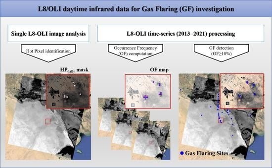
Consequently, the NHI algorithm was rearranged by developing the “Daytime Approach for gas Flaring Investigation” (DAFI) method. This method consists of a three-module cascade shown in
Figure 2, where “HP
daily” refers to hot pixels identified using the condition
II of
Table 2. Equation (4) is used to sum up the HP
daily values and compute the OF for each pixel.
Hence, DAFI works on a single OLI scene searching for hot pixels through the NHI
SWNIR index and the test on saturated pixels in the SWIR1 band (see module
(a)). This operation was performed for all the scenes of the time series, preserving the “detection history” of each location. The OF was calculated from the HP
daily masks and the number of analyzed images, summed in the investigated time window. Pixels showing OF values ≥ 10% were classified as gas flares (module
(b)). Finally, the persistence level of each GF was computed through a quartiles analysis, which allowed us to define four GF persistence levels (module
(c)), shown in
Table 3. The lower the level, the less persistent the activity.
4. Results
The DAFI inventory consists of 1711 high-temperature gas flaring sites, identified over the period 2013–2021 (see
Figure 3).
The distribution of the global GF sites is spatially concentrated: 1237 points are located onshore (72%), while the remaining 474 (28%) were flagged offshore. About 70% of the onshore GFs belongs to Asia (~50%, located in Russian Federation, Iran and Iraq), and ~15% to Africa (Algeria, South Africa) and Americas (United States of America, Mexico, Venezuela). The distribution of the global offshore GFs is concentrated into the North Sea (~9%), Gulf of Guinea (~22%), Persian Gulf (~15%) and South China Sea (~20%); they represent about ~67% of the total [
30]. As far as both onshore and offshore GFs are considered together, the Asia continent is the most populated (
Figure 3), followed by the American and African ones, where GF sites show a quite similar distribution in both offshore and onshore conditions. Europe and Oceania have a marginal role in terms of oil and gas facilities (less than ~15% and ~5%, respectively).
The countries more affected by the gas flaring sites, selected as the ones accounting for at least the 50% of overall continental detections, are listed in
Figure 4.
The Russian Federation, Iran and Iraq occupy the podium, accounting for about 40% of the worldwide detected GFs, followed by Algeria, Mexico and USA. These results are in good agreement with the last report of the Global Gas Flaring Reduction Partnership [
8], stating that Russia, Iraq, Iran, the United States, Algeria, Venezuela and Nigeria are among the top 10 flaring countries. The latter have held this position consistently for the last 10 years, accounting for roughly two-thirds (65%) of global gas flaring.
Figure 5 shows the distribution of the persistence levels for both onshore and offshore GFs categories, emphasizing their different behavior in terms of operability.
In particular, the figure reveals that while the onshore sites have a mid–low persistence, the marine platforms are the most operational, with about 50% of them belonging to the high-persistence class.
Flaring may occur in the oil and gas industry for many reasons, ranging from initial start-up testing of a facility to unplanned equipment malfunctions. The combustion in gas flares can be almost constant over the time, but can also be very variable, hence the flaring can be reduced or turned off. Moreover, a gas flare may be located on a sea platform or on the ground flares with open pits and multiple nozzles, and elevated individual stacks [
33]. All these features affect the time duration of the process, which needs to be considered for detection purposes. Thus, thermal anomalies identified on each site by DAFI have been temporally disaggregated, on an annual and monthly basis, to acquire some information about the source type (i.e., continuous or non-continuous flaring). Some examples are shown in
Section 5.
In sum, the DAFI results, retrieved from daytime L8-OLI data, provide an accurate information about the global distribution, localization and mapping of the most intense gas flaring sites.
5. The DAFI Website
The first level (named “The global gas flaring DAFI map”) allows users to visualize the spatial distribution of the gas flaring sites, navigating a custom map created using Google My Maps (
Figure 6). By clicking on the single site of interest, the following information appears on the left-side of the map (
Figure 6):
- -
Continent, region, country;
- -
GF site longitude and latitude (in decimal degree format);
- -
Occurrence Frequency, OF (%);
- -
Long-term Persistence Level (from low to high, depending on the OF value);
- -
Shore (gas flare location, classified in onshore and offshore).
An identification code is assigned to each gas flaring site. It consists of the country acronym (i.e., Alpha-3 country code) followed by a 4-digit progressive number (e.g., DZA_0357, see example in
Figure 6).
The dynamic characterization of the GF sites runs automatically in GEE. A schematic picture of the developed DAFI App is shown in
Figure 7.
By approaching this level, named “The DAFI App for gas flaring thermal investigation”, two steps are required to investigate the gas flaring source:
- (1)
Choose the gas flare to inspect.
- (2)
Run the DAFI to get the GF behavior. As previously mentioned, by exploring the map, users can select the gas flare of interest. By directly obtaining the ID number (in the drop-down menu) or copying/tasting it from the map the time series of SWIR1 and NIR radiances, measured over the selected GF site, is displayed. Thermal anomalies that are aggregated both in terms of years and months (i.e., OF value during a given calendar year/month), can be visualized through line charts, highlighting the periods in which the thermal activity was dominant, increased or declined at site level. Each graph can be downloaded in CSV, SVG or PNG format.
Some examples of the tool outputs are shown below and refer to both onshore and offshore sites (
Figure 6). The criterion adopted to select them is the following:
This analysis may provide interesting information about differences/similarities in the GF dynamics and thermal behavior. For each site, a picture displaying the GF-affected area (white circle), with the thermally anomalous pixels, depicted in different colors according to their OF value, is shown, along with the annual and monthly temporal profile chart of the GF occurrence.
Figure 8 displays the GF sites belonging to the first aforementioned category (i.e., mid–high): DZA_0313 and RUS_1310.
Figure 8 shows that some differences characterize the GFs sites within the same long-term persistence class. The Algerian gas flare (DZA_0313), with a 12-pixel cluster (
Figure 8a), seems to operate with an increasing trend (with percentages of occurrence lower than 22%) up to 2019, where the peak is recorded (~61%), followed by a reduced continuity in the next two years (see
Figure 8b, purple line). The Russian site (RUS_1310), composed by three pixels (
Figure 8c), shows a quite stable flaring activity between 2013–2018, apart from a slight peak recorded in 2015 (
Figure 8b, purple dashed line), while it halves in the following years. Additionally, at the monthly scale, the OFs distribution of the two sites follows an opposite trend, which is a convex trend for the Algerian flare and quite concave for the Russian one (see
Figure 8d).
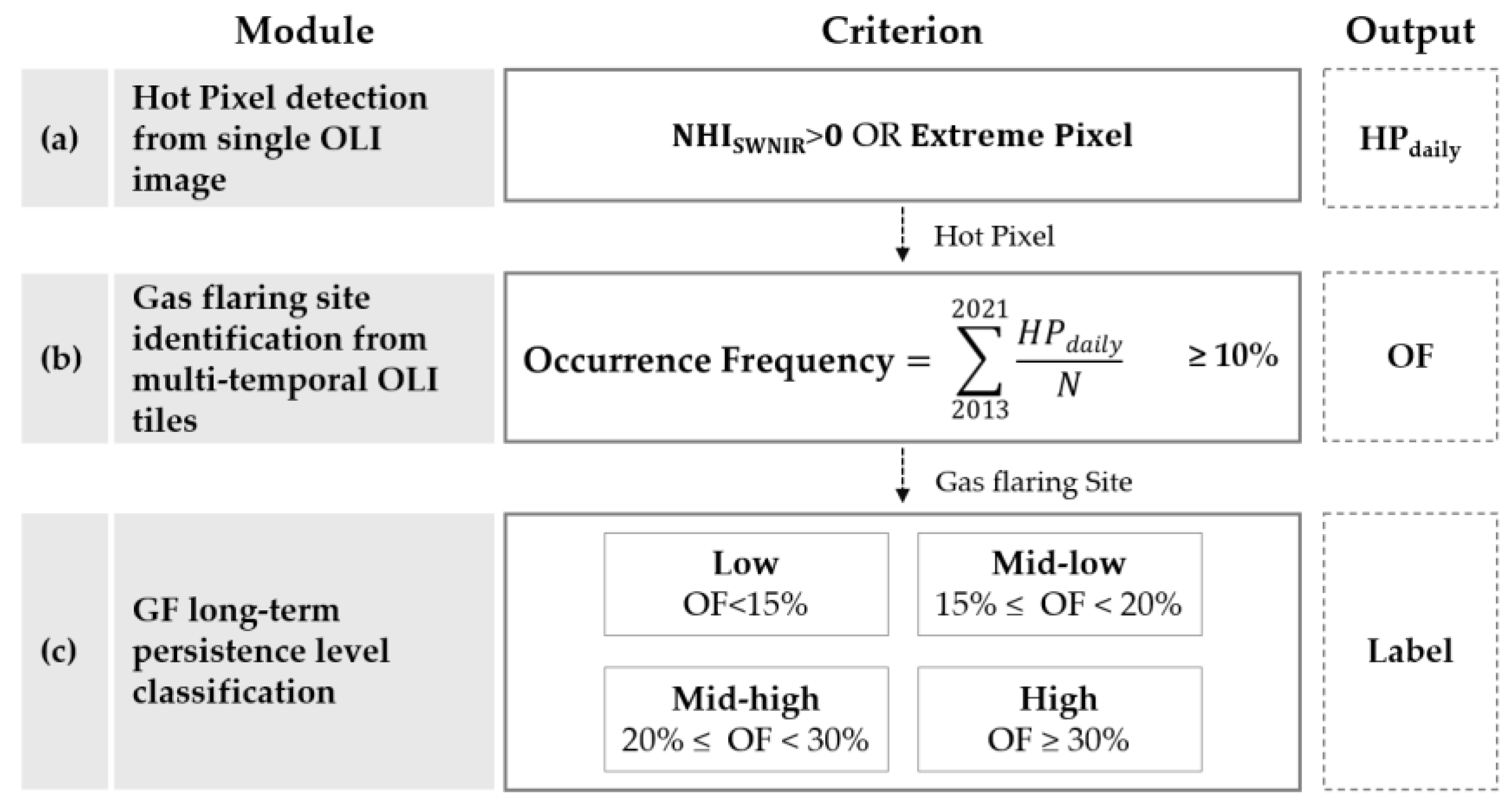
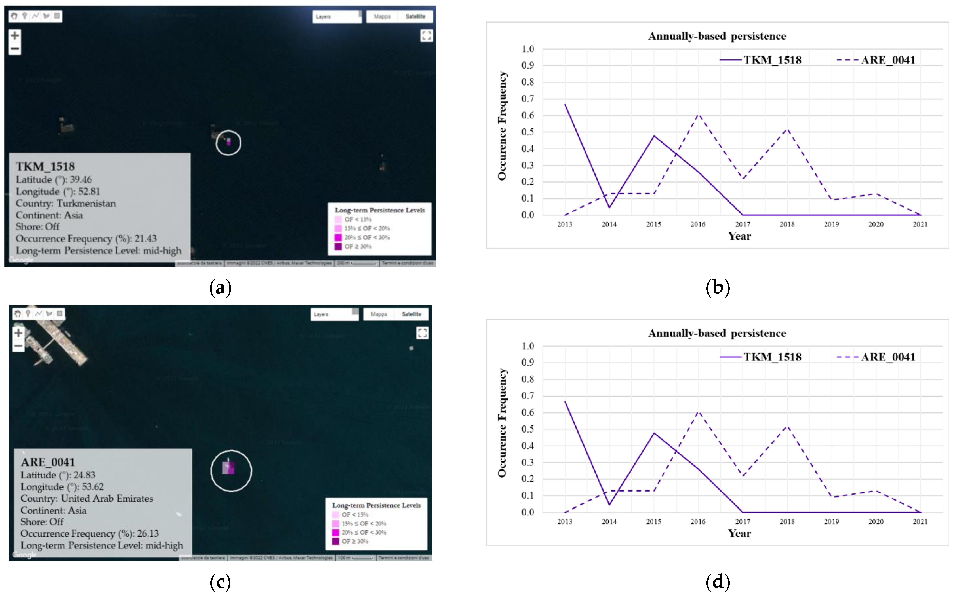
By looking at the selected offshore gas flaring sites, both are classified as mid–high persistence objects (
Figure 9), located in the Caspian Sea (TKM_1518,
Figure 9a) and Persian Gulf (ARE_0041,
Figure 9c), 30 km and 70 km from the Turkmen and United Arab Emirates shores. Both the marine platforms, part of a flaring sites archipelago, are clearly visible from space.
The oil and gas platform in the Caspian Sea has not been operational since 2017 (purple line in
Figure 9b), with an unstable operation in the previous years. The gas flaring has been routinely practiced at the ARE_0041 (purple dashed line in
Figure 9b) from 2014 to 2020, with two peaks in 2016 and 2018. As the previous one, it stopped in 2021. At a monthly scale (
Figure 9d), the two sites work over the whole 12-month period (except in March for TKM_1518), with a higher persistence level for the Arab platform in most of the months (higher than 10%).
Regarding the second category detailed above, the Iraqi sites, IRQ_0795 and IRQ_0766, flagged, respectively, as high and low long-term persistence sources (the cluster size likely reflects this), are represented in
Figure 10a,c.
As highlighted by the line chart in
Figure 10b, the level of annual persistence is significantly different between the two sites over the analyzed years (with a mean bias of 50%). Moreover, observing the IRQ_0795 “high” source, its persistence is gradually increasing during the first four years (2013–2016), with a growth rate of over 70% (the peak is reached in 2016, around 83%) (
Figure 10b, purple line). Since 2016, the level declines for touching the starting one in 2018, when a new rise is recorded. IRQ_0766 appears quite stable, with OF percentages ranging from 5% to 20% over the years 2013–2019, with a peak of 30% in 2020 (
Figure 10b, purple dashed line). The monthly profiles of the Iraqi sites’ occurrences (
Figure 10d) indicate that the gas flaring activity mainly occurs between September and February/March. As expected, the most intense levels (more than 50% on average) can be observed in correspondence with the “high” source.
Figure 10d puts in evidence the same concave trend also characterizing the Algerian and Russian sites (see
Figure 8d). Further investigations are required to better explain those observations.
6. Conclusions
DAFI uses a temporal persistence criterion, applied to a customized NHI-based indicator, to identify the GF sites which were active over the last nine years (i.e., 2013–2021). This way, DAFI is capable of detecting very intense and persistent gas flaring sources, allowing for a deep characterization, in terms of temporal dynamics (at both annual and monthly scale) and spatial spreading of hot pixels at the local scale.
As a final result, the first global map of high-temperature gas flaring sites based on daytime OLI-L8 observations was produced. A GF detection reliability of 99% was achieved by setting the 10% threshold persistence.
It should be pointed out that DAFI information is not exhaustive, owing to the imposed restrictions (see
Section 3). Indeed, while commission errors, associated only with other industrial plants, are negligible and do not represent an issue, the GF database mainly includes the high-temperature gas flares operating in time. In particular, missed detections may occur in the presence of mid–low intensity flares (e.g., GF operating at lower temperatures, and emitting more strongly in the SWIR2 than SWIR1 band) and/or of extremely recent (or presently dismissed) flares, which do not meet the selected criteria (i.e., OF slightly less than 10%). Both factors may affect the completeness of the GF dataset. Moreover, these cases may be further emphasized in case of cloud cover, which hinders or masks the gas flare signals (especially the less intense ones). Moreover, the temporal investigation of the GF occurrence frequency may be misunderstood in geographic areas where clouds persist in some months of the year. In such a case, a measured null (or very small) value of OF maynot be directly related to the gas flare operational features but to the cloud coverage, preventing an effective gas flare site characterization in time domain.
Despite those limitations, the DAFI global daytime map may provide additional information about GFs when integrated with the nighttime VIIRS observations.
Figure 11 displays the spatial distribution of the GFs from the nighttime VNF method, independently provided by the EOG, and the daytime DAFI one.
A general satisfying spatial agreement between daytime and nighttime GF datasets is evident, with the flaring regions identified by DAFI which are also captured by VNF. However, the different spatial resolution, revisit interval, acquisition time and spectral bands used by the two methods make a point-by-point comparison between them impracticable (and even out of the scope of this work). On the other hand, their integration may represent an added value in terms of detection, monitoring and characterization capabilities of GF from space. Indeed, daytime and nighttime observations, if integrated, by increasing the temporal sampling, may allow for a more effective identification of the GFs. Moreover, the different GF typology and characteristics may be better revealed when different spectral/spatial and temporal domains are investigated. A visual investigation of DAFI and VNF maps has revealed relative performance and limitations, as put in evidence by some examples reported in
Figure 12 showing:
- o
The higher sensitivity of OLI to small-scale hot targets, undetected by VIIRS (e.g.,
Figure 12a);
- o
The greater spatial accuracy offered by OLI than VIIRS in localizing and mapping the GF areas, useful information for accurately characterizing the site in terms of flared volumes and GHG emissions (
Figure 12b);
- o
The lower sensitivity of DAFI than VNF in detecting some GFs because of the selected persistence threshold (
Figure 12c) (shale oil/gas included).
Figure 12 clearly shows the advantage of a gas flaring mapping from a complementary satellite-based inventory.
The current DAFI map will be updated annually to follow the GF spatiotemporal dynamics. While the aforementioned limitations probably led to an underestimation of gas flares in this study, they will be likely (at least partially) overcome by exporting DAFI on additional satellite data at mid–high spatial resolution. In particular, the DAFI porting on Landsat 9 and Sentinel 2A/B (at 20m spatial resolution) data is under development, by taking into account the preliminary outcomes shown in [
21]. The combination of Sentinel-2A/B MSI and L8/9 OLI/OLI-2 data would guarantee an increased frequency of observation, up to a revisit time of 1–3 days [
34,
35,
36,
37], with a positive impact on the detection sensitivity. The OF percentage levels lower than 10% will also be explored using L9 and S2 collections. Moreover, the different behavior of the onshore and offshore sites, observed by applying the long-term persistence class, will be better analyzed, evaluating the DAFI performance in recognizing hot pixels over different areas. Estimates of the radiative power, for each gas flare, will be also performed and made available on the DAFI website. This metric will be crucial to carefully retrieve both the volume of gas flared and the CO
2 equivalent emissions by each identified GF over one calendar year/month.
Given the growing international focus on global methane emissions, and acknowledging the important role the oil and gas industry could play towards achieving climate goals [
8], a global overview of the GF sites, as exhaustive as possible, becomes crucial for monitoring the countries’ progress in decarbonization strategies [
8].
Considering that bottom-up emission inventories for the oil and gas industry are often fragmentary, due to challenges in quantifying the emissions from gas flaring or to incomplete reporting by individual companies, satellite-based observations may then be offering a valuable alternative to independently acquire more complete, accurate and timely emission estimates [
7].
A global GF emissions scenario that is as exhaustive as possible may help governments and operators in tracking commitments and efforts in oil-producing countries to abate flaring, as well as in conducting air quality monitoring for better understanding of exposures, and reducing potential human health impacts [
31,
38].


