A Hybrid-Order Spectral-Spatial Feature Network for Hyperspectral Image Classification

Abstract

Convolutional neural networks are widely applied in hyperspectral image (HSI) classification and show excellent performance. However, there are two challenges: the first is that fine features are generally lost in the process of depth transfer; the second is that most existing studies usually restore to first-order features, whereas they rarely consider second-order representations. To tackle the above two problems, this article proposes a hybrid-order spectral-spatial feature network (HS²FNet) for hyperspectral image classification. This framework consists of a precedent feature extraction module (PFEM) and a feature rethinking module (FRM). The former is constructed to capture multiscale spectral-spatial features and focus on adaptively recalibrate channel-wise and spatial-wise feature responses to achieve first-order spectral-spatial feature distillation. The latter is devised to heighten the representative ability of HSI by capturing the importance of feature cross-dimension, while learning more discriminative representations by exploiting the second-order statistics of HSI, thereby improving the classification performance. Massive experiments demonstrate that the proposed network achieves plausible results compared with the state-of-the-art classification methods.

1. Introduction

A hyperspectral image (HSI), which is generally captured by imaging spectrometers or hyperspectral remote sensing sensors, comprises hundreds of narrow spectral bands and abundant spatial distribution information [1,2]. Because of rich spatial and spectral information, HSI has been widely applied in various fields, such as mineral exploitation [3], environmental science [4], military defense [5], urban development [6]. HSI classification, which aims to assign an accurate ground-truth label to each hyperspectral pixel, has become a hot topic in the field of remote sensing in recent years [7,8,9,10].

In the initial phase, a substantial number of classification methods using machine learning (ML) were presented. These methods usually perform feature extraction and then feed the obtained features into classifiers [11], such as support vector machine (SVM) [12], multinomial logistic regression [13] or random forest [14], for training. Yuan et al. utilized the cluster method to split spectral bands into several sets and selected important bands to accomplish classification tasks [15]. An SVM with nonlinear kernel projection method was proposed [16]. The Markov random field (MRF) was combined with band selection for classification [17]. However, these traditional spectral features-based classification methods do not fully exploit the spatial information of HSI. Therefore, certain classification methods based on spectral-spatial features had been proposed to improve HSI classification performance. A set of complex Gabor wavelets were used to capture spectral-spatial features [18]. Li et al. integrated local spatial features, global spatial features and original spectral features for HSI classification [19]. To obtain spectral and spatial information, extended morphological profiles (EMPs) [20], multi-kernel learning (MKL) [21] and sparse representation-based classifier (SRC) [22] introduced spatial information into the training process. He et al. systematically reviewed the conventional spectral-spatial-based classification methods [23]. Paul et al. proposed a particle swarm optimization-based unsupervised Dimensionality reduction method for HIS classification, where spectral and spatial information is utilized to select informative bands [24]. Nevertheless, these HSI classification methods using ML, whether based on spectral features or based on spectral-spatial features, rely on handcrafted features with limited representation ability, which leads to poor representation and generalization ability.

With the breakthrough of deep learning in the field of artificial intelligence, deep learning (DL)-based HSI classification methods have attracted substantial attention and have become a hotspot. Compared with ML-based classification methods, DL-based methods not only extract abstract features from the low level to the high level but also transform images into more recognizable features, which can provide a fine classification result. Typical DL-based methods involve deep belief networks (DBNs) [25], stacked autoencoders (SAEs) [26], recurrent neural networks (RNNs) [27] and convolutional neural networks (CNNs) [28], which greatly enhance the HSI classification performance. Due to the characteristics of local connection and weight sharing, CNNs have been gradually introduced into HSI classification and have shown promising performance. Hu et al. utilized a 1-D CNN to extract spectral information to accurately classify HSI [29]. A unified framework that combined SAM with a CNN was presented to adaptively learn weight features for each hyperspectral pixel by 1-D convolutional layers [30]. However, the input data of 1-D CNN-based methods must be flattened into 1-D vectors, which disregards the rich spatial features of HSI.

To further boost the classification performance, many 2-D CNN-based and 3-D CNN-based methods have been proposed to capture spectral and spatial features. Yang et al. designed a two-CNN to learn the spectral and spatial joint features [31]. Zhang et al. constructed a novel spectral-spatial-semantic network with multiway attention mechanisms for HSI classification [32]. Li et al. built a deep multilayer fusion dense network to obtain the correlation between spectral information and spatial information [33]. A supervised 2-D CNN consisted of three 2-D convolutional layers and a 3-D CNN composed of three 3-D convolutional layers were introduced for classification [34]. Although these classification methods have achieved considerable progress, how to further enhance the HSI classification accuracy with limited training samples is still challenging. Inspired by residual learning [35] and dense connections [36], Meng et al. presented two mixed link networks to obtain more representative features from HSI, aggregating the characteristics of feature reuse and exploration [37]. Paoletti et al. utilized a dense and deep 3-D CNN to take full advantage of HSI information [38]. Li et al. introduced the maximum correntropy criterion to generate a robust 3D-CapsNet [39]. To deal with the spectral similarity between HSI cubes of spatially adjacent categories, Mei et al. built a cascade residual capsule network for HSI classification [40]. To obtained global information and reduced computational cost, Yu et al. designed a dual-channel convolutional network for HSI classification [41]. However, the spectral-spatial features processed by convolutional layers may include much disturbing or unimportant information. Therefore, focusing on necessary informative regions while suppressing useless regions is still an essential problem.

Recently, inspired by the attention mechanism of human visual perception, many effective and classical attention modules have been introduced into CNNs to ameliorate HSI classification performance. Xi et al. designed 3-D squeeze-and-excitation residual blocks in each stream of framework to learn the spectral and spatial features from low level to high level [42]. To obtain a complex spectral-spatial distribution, Feng et al. devised a symmetric GAN by utilizing an attention mechanism and collaborative learning [43]. Sun et al. captured representative spatial and spectral features from the attention regions of image cubes [44]. Ma et al. proposed a double-branch multi-attention mechanism network [45]. Xiang et al. constructed an end-to-end multilevel hybrid attention framework consisting of a 3D-CNN, grouped residual 2D-CNN and coordinate attention [46]. Zhang et al. devised a spectral partitioning residual network with a spatial attention mechanism [47]. Ge et al. introduced an adaptive hash attention mechanism to properly extract the spectral and spatial information [48]. Wang et al. presented a spatio-spectral attention to boost the expression of the important characteristic among all pixels [49]. To enhance the robustness of HSI rotation, Yang et al. designed a cross-attention spectral-spatial network [50]. Although these methods can achieve good classification results, they usually only consider first-order statistical features and rarely learn second-order representations to enhance HSI classification performance.

Modeling of second-order or high-order statistics for obtaining discriminative representations has attracted considerable interest in deep CNNs. In particular, the global second-order pooling can fully utilize the correlation information between different channels, achieving significant performance improvement [51,52,53]. Moreover, the global second-order pooling has attracted much attention in the field of HSI classification. He et al. employed multiscale covariance maps to fully exploit the spectral and spatial information [54]. Zheng et al. proposed a mixed CNN with covariance pooling to integrate spectral and spatial features [55]. Xue et al. designed a novel second-order pooling network based on an attention mechanism [56].

In this paper, motivated by the abovementioned advanced CNN models, we propose a hybrid-order spectral-spatial feature network (HS²FNet) constructed by a precedent feature extraction module (PFEM) and a feature rethinking module (FRM) for hyperspectral image classification. The former is composed of several symmetrical feature extraction blocks (SFEBs) and a distillation block (DB), which captures first-order spectral-spatial features. The latter models more discriminative second-order spectral-spatial representations, which can further refine first-order spectral-spatial features obtained from PFEM, thereby enhancing the classification performance. Specifically, we first design a SFEB to extract spectral-spatial features from different scales and layers. Considering that the connected multiscale features are beneficial for HSI classification, then a DB is built to focus on adaptively recalibrate hierarchical features by strengthening meaningful channels and paying attention to the informative region of spatial dimension, which can eliminate redundant information and achieve first-order feature distillation. Furthermore, to improve classification accuracy, we design a FRM to model more representative second-order spectral-spatial features, which introduces the importance of feature cross-dimension and the second-order statistics of HSI. Finally, we utilize two fully connected layers, two dropout layers and a soft-max layer to perform classification.

The main contributions of this paper are summarized as follows:

• We design a symmetrical feature extraction block to capture spectral-spatial features from different scales and layers, while maximizing the use of HSI feature flows between different scales.
• To dispel redundant information and noise, a distillation block is devised, which can focus on adaptively recalibratin channel-wise and spatial-wise feature responses to achieve first-order spectral-spatial feature distillation.
• We build a feature rethinking module to model more discriminative second-order spectral-spatial features, which further refines the first-order features by capturing the importance of feature cross-dimension and improving the classification performance by exploiting the second-order statistics of HSI, thereby improving the classification performance.

The rest of this paper is organized as follows. In Section 2, we introduce the proposed hybrid-order spectral-spatial feature network in detail. In Section 3, the experimental results and discussion are presented. Finally, the conclusion and future research direction are given in Section 4.

2. Method

The overall structure of the proposed network using the Indian Pines (IP) dataset as an example is illustrated in Figure 1. This work utilizes the precedent feature extraction module (PFEM) to obtain first-order spectral-spatial information. PFEM consists of several symmetrical feature extraction blocks (SFEBs) and a distillation block (DB). The feature rethinking module (FRM) is employed to model more discriminative second-order spectral-spatial representations. FRM can further refine and sublimate first-order spectral-spatial features captured by the PFEM, thereby boosting accurate and efficient classification.

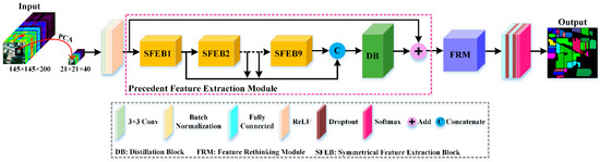
Figure 1. Overview of the presented HS²FNet for HSI classification.

In Figure 1, a PCA transformation is first applied on the raw HSI to retain important spectral bands and effectively downsize the memory capacity required for calculation. To make full use of the property of HSI, we extract a 3-D image cube of size $21\times 21\times 40$ as the input of our proposed method. Then, the $21\times 21\times 40$ image cube is sent to the initial module including a $3\times 3$ convolutional layer, a batch normalization (BN) layer and a rectified linear unit (ReLU) to obtain the general feature maps. Furthermore, the acquired feature maps are fed into nine cascaded SFEBs to detect multiscale spectral-spatial features. The multiscale spectral-spatial contextual information is beneficial for HSI classification. However, if the multiscale features obtained from nine SFEBs are only simply concatenated together, this may introduce some noises and unnecessary information. Therefore, we design a DB to focus on adaptively recalibrating hierarchical features by strengthening meaningful channels and paying attention to the informative region of the spatial dimension. Next, the first-order hierarchical distillation features are transmitted to FRM to acquire more discriminative second-order representations by capturing the importance of features’ cross-dimension and exploiting the second-order statistics of HSI. Finally, classification is performed through two fully connected layers, two dropout layers and a soft-max layer. More details on PFEM and FRM are provided next.

2.1. Precedent Feature Extraction Module

Spectral-spatial feature extraction is the most crucial step for HSI classification, the features obtained from different layers have different characteristics. Low-level features have higher resolution and contain more details but are full of noise, while high-level features have stronger semantic information but lack the perception capability for details. Low-level and high-level features are complementary, and the combination of the two is helpful for HSI classification. Therefore, we build a SFEB to capture multiscale spectral-spatial features and maximize the use of HSI feature flows at different scales. Multi-level features are significantly different to each other, and taking full advantage of hierarchical spectral-spatial features is also vital for HSI classification. Unfortunately, hierarchical features may bring some noise and redundant information, which will make the network more difficult to train and degree the classification performance. To address this problem, we design a DB which can effectively utilize hierarchical features while dispelling noise and redundant information, thereby achieving first-order spectral-spatial feature distillation.

2.1.1. Symmetrical Feature Extraction Block

With the development of DL networks, a progressive structure named DenseNet is proposed to alleviate the problems of overfitting and gradient vanishing [36]. Specifically, the feature maps learned by all layers are connected one by one and input into all subsequent layers, which can enhance information flows. ResNet can be built by stacking micro-blocks sequentially, which not only solves the degradation problem but also increases training speed [35]. Many studies have proved that making the most of multiscale spectral-spatial features can effectively improve HSI classification performance [57,58,59]. Inspired by the above advantages of DL networks, we raise a SFEB comprising three parts: a symmetrical multiscale dense link unit to integrate spectral-spatial features from different scales and layers, cross transmission to facilitate the propagation of information between different scales, and local skip transmission to avoid unnecessary loss of previous features. The proposed SFEB is provided in Figure 2.

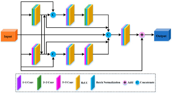
Figure 2. The structure of the symmetrical feature extraction block (SFEB).

Symmetrical Multiscale Dense Link Unit

As shown in Figure 2, SFEB utilizes two different convolutional kernels to acquire different scale spectral-spatial features, including $3\times 3$ and $5\times 5$. To better explain the working mechanism, we divide the SFEB into two parts: Top-Link unit and Bottom-Link unit. Top-Link unit and Bottom-Link unit can not only reduce the depth of network but also apply $1\times 1$ convolutional layers for feature fusion. The operations of Top-Link unit can be expressed as follows:

$$S_1={\omega }_{3\times 3}^1\ast M_{n-1}$$

(1)

$$S_2={\omega }_{3\times 3}^2\ast ({\omega }_{1\times 1}^2\ast [M_{n-1},S_1])$$

(2)

$$Z_{\mathit{sout}}={\omega }_{1\times 1}^3\ast [M_{n-1},S_1,S_2]$$

(3)

where $M_{n-1}$ and $Z_{\mathit{sout}}$ denote the input and output of Top-Link unit, respectively. $\omega$ stands for weights of convolution layer. The superscripts refer to the number of layers at which they are located. The subscripts refer to the size of convolutional kernel used in this layer. $[M_{n-1},S_1]$ and $[M_{n-1},S_1,S_2]$ are concatenation operation.

To obtain different scale spectral-spatial features, we use $5\times 5$ convolutional layers instead of all $3\times 3$ convolutional layers in the Bottom-Link unit. The operations of Bottom-Link unit can be expressed as follows:

$$P_1={\omega }_{5\times 5}^1\ast M_{n-1}$$

(4)

$$P_2={\omega }_{5\times 5}^2\ast ({\omega }_{1\times 1}^2\ast [M_{n-1},P_1])$$

(5)

$$Z_{\mathit{pout}}={\omega }_{1\times 1}^3\ast [M_{n-1},P_1,P_2]$$

(6)

where $M_{n-1}$ and $Z_{\mathit{pout}}$ denote the input and output of Bottom-Link unit, respectively. $[M_{n-1},P_1]$ and $[M_{n-1},P_1,P_2]$ are the concatenation operation.

Cross Transmission

The transfer and fusion of features at different scales has a big impact on feature extraction. Therefore, we introduce the cross transmission into Top-Link unit and Bottom-Link unit, which can transmit different scale spectral-spatial features by themselves to other subsets. Moreover, to reduce dimension and achieve multiscale spectral-spatial features fusion, we employ a $1\times 1$ convolutional layer. The complete operations of cross transmission and feature fusion can be described as follows:

$$S_1={\omega }_{3\times 3}^1\ast M_{n-1}$$

(7)

$$P_1={\omega }_{5\times 5}^1\ast M_{n-1}$$

(8)

$$S_2={\omega }_{3\times 3}^2\ast ({\omega }_{1\times 1}^2\ast [M_{n-1},S_1,P_1])$$

(9)

$$P_2={\omega }_{3\times 3}^2\ast ({\omega }_{1\times 1}^2\ast [M_{n-1},P_1,S_1])$$

(10)

$$Z_1={\omega }_{1\times 1}^3\ast [S_2,S_1,M_{n-1},P_1,P_2]$$

(11)

where $M_{n-1}$ and $Z_1$ denote the input and output of SFEB, respectively. The cross transmission and feature fusion can facilitate the exchange of spectral-spatial features at different scales and achieve multiscale feature fusion.

Local Skip Transmission

We also introduce local skip transmission into our constructed SFEB to achieve reasonable feature reuse and strengthen information propagation. The output of SFEB can be written as follows:

$$M_n=M_{n-1}+Z_1$$

(12)

2.1.2. Distillation Block

During the training process, spectral-spatial features will gradually disappear with the increase in network depth. Therefore, fully exploiting concatenated features is conducive to improve classification accuracy. However, only using $1\times 1$ convolutional layers to concatenate and compress these hierarchical features may produce massive redundant information and be adverse to HSI classification. In this section, we present a DB to effectively utilize hierarchical spectral-spatial features and achieve first-order feature distillation. DB consists of two principal branches: channel-wise recalibrate branch and spatial-wise recalibration branch. The former adaptively recalibrate channel-wise features by strengthening meaningful channels. The latter adaptively recalibrate spatial-wise features by paying attention to the informative regions of spatial dimension. The proposed DB is provided in Figure 3.

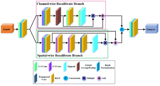
Figure 3. The structure of the distillation block (DB).

As shown in Figure 3, first, to reduce the number of feature maps without losing fine features, we introduce two $1\times 1$ convolutional layers at the head and tail of DB, respectively. Then, DB splits the spectral-spatial features obtained from the first $1\times 1$ convolutional layer into two branches, i.e., channel-wise recalibrate branch and spatial-wise recalibrate branch. Finally, we employ a simple concatenation operation to integrate the two branches into one new group.

Feature Splitting

The input spectral-spatial features of DB are denoted as $X\in R^{H\times W\times g}$, where $H$ and $W$ refer to the height and width of the spatial dimension, respectively, and $g$ represents the number of channels. The DB divides $X$ into two branches along the spectral dimension, where $X=[x_1,x_2], x_1 \mathit{and} x_2\in R^{H\times W\times (g/2)}$, and channel-wise recalibrate branch and spatial-wise recalibrate branch are denoted $x_1$ and $x_2$, respectively.

Channel-Wise Recalibrate Branch

To refine the channel weights of spectral-spatial feature maps, we design a channel-wise recalibrate branch. The network structure of the proposed channel-wise recalibrate branch is shown in Figure 3. First, the global average pooling is utilized to average the spatial dimension of feature maps to obtain feature maps with a size of $1\times 1\times (g/2)$. Second, the feature tensors are sent to a $1\times 1$, $(g/2)/r$ 2-D convolutional layer to reduce the channel dimension and focus on the meaningful channels, where $r$ is the channel compressed ratio. Then, we use a ReLU activation layer to strengthen the nonlinear relationship of channels. Next, a $1\times 1$, $g/2$ 2-D convolutional layer is utilized to increase the channel dimension and obtain the $g/2$ spectral-spatial feature maps. Finally, we apply a sigmoid function to limit the range of features, and the original output features are multiplied by the weight coefficients to obtain the refined channel features.

Spatial-Wise Recalibrate Branch

To pay attention to the informative regions of spatial dimension, we propose a spatial-wise recalibrate branch. The network structure of the proposed spatial-wise recalibrate branch is shown in Figure 3. First, we utilize two 2-D convolutional layers with C filters of $3\times 3$ size and a $2\times C$ filters of $3\times 3$ size to reduce the spatial dimension of features to obtain the feature maps involving important location information. Then, two transposed convolutional layers with C filters of $3\times 3$ size are introduced to restore the original size. The transposed convolutional layer can not only maintain the mapping relationship of spatial locations but also be vital for the subsequent weight optimization process. Here, each convolutional layer is followed by a ReLU activation function, which is used to enhance the nonlinear correlation. Finally, a sigmoid activation function is applied to limit the spectral-spatial feature maps to $[0,1]$ range, and the output is multiplied with the feature maps to guarantee that the input of next layer is optimal.

2.2. Feature Rethinking Module

Recently, the global second-order pooling operation has been widely applied in a variety of vision tasks and achieved significant performance improvement [60,61,62]. The global second-order pooling can not only learn second-order representations but also enhance nonlinear modelling capability of a network. Inspired by the above advantages of global second-order pooling, we design an FRM to model more discriminative second-order spectral-spatial feature representations by capturing the importance of feature cross-dimension and exploiting the second-order statistics of HSI. To better explain the working mechanism, we divide the FRM into two parts: feature cross-dimension interaction (FCI) and second-order pooling (SP). The proposed FRM is provided in Figure 4.

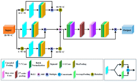
Figure 4. The structure of the feature rethinking module (FRM).

2.2.1. Feature Cross-Dimension Interaction

FCI is applied to capture close interdependencies between the $(H,W)$, $(H,C)$ and $(W,C)$ dimensions of HSI, respectively, further enriching spectral-spatial feature representations. The diagram of FCI is provided in Figure 4. FCI is composed of three parallel streams: cross-dimension dependency between the spatial dimension $H$ and the channel dimension $C$, dependency between the spatial dimension $H$ and the spatial dimension $W$, and cross-dimension dependency between the spatial dimension $W$ and the channel dimension $C$.

Cascaded Pooling

The cascaded pooling is made up of max-pooling features and average-pooling features to reduce the second dimension of the image cube. Mathematically, it can be expressed by the following equation:

$$\mathit{cascaded} \mathit{pooling}(X)=[\mathit{Maxpool}(X), \mathit{Averagepool}(X)]$$

(13)

where the second dimension across takes place during the max-pooling and average-pooling operations. For example, the size of the image cube is $(H,W,C)$, and the output size of the cascaded pooling is $(H,W,2)$. The cascaded pooling can not only ease computational overhead but also preserve an affluent spectral-spatial feature representation.

Triplet Cross-Dimension Stream

The input tensor of FCI are denoted as $X\in R^{H\times W\times C}$, where $H$ and $W$ represent the height and width of the spatial domain, respectively, and $C$ refers to the number of channel. We transmit $X$ to each stream of the proposed FCI. In the first stream, we capture interdependency between the spatial dimension $H$ and the channel dimension $C$. First, we rotate $X$ $90°$ anti-clockwise along the $H$ axis to obtain the rotated tensor $X_1$ whose shape is $H\times C\times W$. Second, $X_1$ is sent to the cascaded pooling to reduce the second dimension of $X_1$. The gotten reduced dimension result is denoted as ${\tilde{X}}_1$, which is of shape $H\times C\times 2$. Subsequently, ${\tilde{X}}_1$ is entered into a 2-D convolutional layer with 1 filter of $7\times 7$ size followed by a BN layer, which provides the intermediate output of shape $H\times C\times 1$. Then, a sigmoid function is utilized to generate attention weights. Finally, the obtained attention weights are multiplied by $X_1$ and then rotated $90°$ clockwise along the $H$ axis to remain the same shape as input $X$.

For the second stream, we acquire interdependency between the spatial dimension $H$ and the spatial dimension $W$. First, the channels of $X$ are reduced to two by the cascaded pooling. Then, the obtained reduced dimension tensor ${\tilde{X}}_2$ of shape $H\times W\times 2$ is sent to a 2-D convolutional layer with 1 filter of $7\times 7$ size followed by a BN layer. Finally, the output is passed through a sigmoid function to generate attention weights of shape $H\times W\times 1$ which are applied to the input $X$.

Similarly, in the third stream, we achieve interdependency between the spatial dimension $W$ and the channel dimension $C$. First, we rotate $X$ $90°$ anti-clockwise along the $W$ axis to obtain the rotated tensor $X_3$, whose shape is $C\times W\times H$. Second, $X_3$ is sent to the cascaded pooling to reduce the second dimension of $X_3$. The achieved dimension result is denoted as ${\tilde{X}}_3$, which is of shape $C\times W\times 2$. Subsequently, ${\tilde{X}}_3$ is entered into a 2-D convolutional layer with 1 filter of $7\times 7$ size followed by a BN layer, which provides the intermediate output of shape $C\times W\times 1$. Then, a sigmoid function is utilized to generate attention weights. Finally, the obtained attention weights are multiplied by $X_3$ and then rotated $90°$ clockwise along $W$ axis to remain the original input shape of $X$.

The tensors with FCI of shape $H\times W\times C$ generated by each stream are aggregated by element-wise summation, and then we utilize a simple average operation to obtain the final refined output. The process of FCI can be summarized as follows:

$$y_1=X_1\times \sigma ({\omega }_1\ast {\tilde{X}}_1)$$

(14)

$$y_2=X\times \sigma ({\omega }_2\ast {\tilde{X}}_2)$$

(15)

$$y_3=X_3\times \sigma ({\omega }_3\ast {\tilde{X}}_3)$$

(16)

$$y=\frac{1}{3}({\overline{y}}_1+y_2+{\overline{y}}_3)$$

(17)

where ${\omega }_1$, ${\omega }_2$ and ${\omega }_3$ represent the weights of 2-D convolutional layers in the three streams, respectively. $\sigma$ denotes the sigmoid activation function. $y_1$, $y_2$ and $y_3$ are the output of the three streams, and y is the output of FCI. ${\overline{y}}_1$ and ${\overline{y}}_3$ refer to the ${90}^{\circ }$ clockwise rotation to remain the original input shape of $H\times W\times C$.

2.2.2. Second-Order Pooling

Figure 4 provides the structure of SP. Similar to the squeeze-and-excitation networks [63], SP includes the squeeze process and the excitation process. The squeeze process aims to extract the global second statistics along the channel dimension of the input tensor. Given an input tensor $X\in R^{H\times W\times C}$, to lessen the computational cost, we first pass it to a 2-D convolutional layer of $1\times 1$ size to reduce the number of channels from $C$ to $d$. Second, for the reduced dimension tensor, pairwise channel correlations are computed to gain one $d\times d$ covariance matrix. In the excitation process, due to the order of data being changed by the quadratic operations, we employ a row-wise convolution to remain the inherit structural information for the covariance matrix. Then, a 2-D convolution operation is performed, and we utilize the sigmoid activation function to obtain a $1\times 1\times d$ weight vector. Finally, the corresponding element in the weight vector is multiplied by each channel of $X$. SP pays attention to the correlation between spectral and spatial locations, while taking full advantage of HIS information to obtain more representative second-order spectral-spatial features.

3. Experiments and Discussion

The experimental setup, experimental parameter settings, framework parameter settings, comparisons with the state-of-the-art method, generalization performance and ablation studies are described and discussed here in detail.

3.1. Experiment Setup

3.1.1. Datasets

Four public HSI datasets are used in our experiments to evaluate qualitatively and quantitatively the classification performance of the proposed HS²FNet.

The University of Pavia (UP) dataset [44] including nine ground-truth categories was collected by a Reflective Optics System Imaging Spectrometer (ROSIS-03) over the Pavia region of northern Italy with a spatial resolution of 1.3 $\mathrm{m}$ per pixel $(\mathrm{mpp})$. It is composed of 103 bands ranging from 0.43 to 0.86 $\mathsf{\mu }\mathrm{m}$ and $610\times 340$ pixels. The experiments use the number of training and test samples of the UP dataset is summarized in Table 1.

Table 1. Number of training and test samples of UP dataset.

No.	Color	Class	Train	Test
1		Asphalt	664	5967
2		Meadows	1865	16,784
3		Gravel	210	1889
4		Trees	307	2757
5		Metal sheets	135	1210
6		Bare Soil	503	4526
7		Bitumen	133	1197
8		Bricks	369	3313
9		Shadows	95	852
	Total		4281	38,495

The Kennedy Space Centre (KSC) dataset [64] containing 13 ground-truth categories was acquired by an airborne Visible/Infrared imaging spectrometer (AVIRIS) at the Kennedy Space Centre in Florida. The spatial resolution is 18 $\mathrm{mpp}$. It comprises $512\times 614$ pixels and 176 bands ranging from 0.4 to 2.5 $\mathsf{\mu }\mathrm{m}$. The experiments use the number of training and test samples of the KSC dataset is summarized in Table 2.

Table 2. Number of training and test samples of KSC dataset.

No.	Color	Class	Train	Test
1		Scrub	153	608
2		Willow	49	194
3		CP hammock	52	204
4		Slash pine	51	201
5		Oak/Broadleaf	33	128
6		Hardwood	46	183
7		Grass-pasture-mowed	21	84
8		Graminoid marsh	87	344
9		Spartina marsh	104	416
10		Cattail marsh	81	323
11		Salt marsh	84	335
12		Mud flats	101	402
13		Water	186	741
	Total		1048	4163

The Indian Pines (IP) dataset [44] including 16 ground-truth categories was captured by an AVIRIS over the India Pine Forest pilot area of Northwestern Indiana with a spatial resolution 20 $\mathrm{mpp}$. It consists of 200 bands ranging from 0.4 to 2.5 $\mathsf{\mu }\mathrm{m}$ and $145\times 145$ pixels. The experiments use the number of training and test samples of the IP dataset is summarized in Table 3.

Table 3. Number of training and test samples of IP dataset.

No.	Color	Class	Train	Test
1		Alfalfa	10	36
2		Corn-notill	286	1142
3		Corn-mintill	166	664
4		Corn	48	189
5		Grass-pasture	97	386
6		Grass-trees	146	584
7		Grass-pasture-mowed	6	22
8		Hay-windrowed	96	382
9		Oats	4	16
10		Soybean-notill	195	777
11		Soybean-mintill	491	1964
12		Soybean-clean	119	474
13		Wheat	41	164
14		Woods	253	1012
15		Buildings-Grass-Tree	78	308
16		Stone-Steel-Towers	19	74
	Total		2055	8194

The Salinas (SA) dataset [44] containing 16 ground-truth categories was gathered by an AVIRIS sensor over the Salinas Valley of California. The spatial resolution is 3.7 $\mathrm{mpp}$. It includes $512\times 217$ pixels and 204 bands ranging from 0.4 to 2.5 $\mathsf{\mu }\mathrm{m}$. The experiments use the number of training and test samples of the SA dataset as summarized in Table 4.

Table 4. Number of training and test samples of SA dataset.

No.	Color	Class	Train	Test
1		Broccoli-green-weeds-1	201	2825
2		Broccoli-green-weeds-2	373	3353
3		Fallow	198	1178
4		Fallow-rough-plow	140	154
5		Fallow-smooth	268	2410
6		Stubble-trees	396	3563
7		Celery	358	3221
8		Grapes-untrained	1128	10,143
9		Soil-vineyard-develop	621	5582
10		Corn-senseced-green-weeds	328	2950
11		Lettuce-romaine-4wk	107	961
12		Lettuce-romaine-5wk	193	1734
13		Lettuce-romaine-6wk	92	824
14		Lettuce-romaine-7wk	107	963
15		Vineyard-untrained	727	6541
16		Vineyard-vertical-trellis	181	1626
	Total		5418	48,711

3.1.2. Implementation Details

We randomly choose 20% of the samples for the training and the remaining 80% of the samples for the test for the KSC and IP datasets. For the UP and SA datasets, 10% of samples are selected at random for training and the remaining 90% of samples are utilized for testing. Different experimental datasets contain different sample numbers, so they need to set various batch sizes. The batch size of four experimental datasets is 16, 16, 16 and 128, respectively. In addition, our proposed method is trained in 100 epochs, 100 epochs, 100 epochs and 50 epochs for UP dataset, KSC dataset, IP dataset and SA dataset, respectively. In the training process, the optimizer plays an important role and affects the model convergence. To make the model converge rapidly, we utilize Adam as the optimizer. Specifically, the value of learning rate is set as 0.00001 for four experimental datasets.

The hardware environment of the experiments is a server with an NVIDIA GeForce RTX 2060 SUPER GPU and Intel i-7 9700F CPU. In addition, the software platform is based on TensorFlow 2.3.0, Keras 2.4.3, CUDA 10.1 and Python 3.6.

To analyze the classification effect of the proposed method, four commonly used evaluation indicators are adopted: the accuracy of each category, the overall accuracy (OA), the average accuracy (AA), and the kappa coefficient (Kappa). In theory, the closer these evaluation indicators utilized in this paper are to 1, the better the classification performance will be.

3.2. Framework Parameter Settings

The classification performance of our proposed HS²FNet is affected by five important parameters, i.e., different spatial sizes, diverse training percentages, different numbers of principal components, diverse compressed ratios in the DB, and various numbers of SFEBs. In this part, in term of HSI classification results, we discuss the influences of these five parameters under different value settings.

3.2.1. Influence of Different Spatial Sizes

The spatial size of image cube has a relatively large influence on the classification performance of the proposed HS²FNet. The small spatial size will result in that the loss of spectral-spatial information and damage the classification results. The large spatial size will lead to the central pixel of image cube containing the spectral-spatial information proportion being lower, which is not conducive to HSI classification. So, it is vital for HSI classification to choose an appropriate spatial size. In this paper, we adopt different spatial sizes to find the best one for our proposed method, i.e., $15\times 15$, $17\times 17$, $19\times 19$, $21\times 21$, $23\times 23$, $25\times 25$, $27\times 27$, $29\times 29$. The influences of different spatial sizes on four experimental datasets are provided in Figure 5. From Figure 5a,c,d, we can visually see that for the UP dataset, as the spatial size is $15\times 15$, and for the IP dataset and SA dataset, as the spatial size is $21\times 21$, three evaluation indexes are obviously better than the others, which all exceed 99%. Therefore, the spatial size of $15\times 15$, $21\times 21$, $21\times 21$ is chosen as the pertinent image cube of the proposed HS²FNet on UP dataset, IP dataset and SA dataset, respectively. From Figure 5b, as the spatial size is $25\times 25$ or $29\times 29$, three evaluation indexes all are 100%. Considering the training time and computable cost, we regard the spatial size of $25\times 25$ as the most suitable input of our proposed method for the KSC dataset.

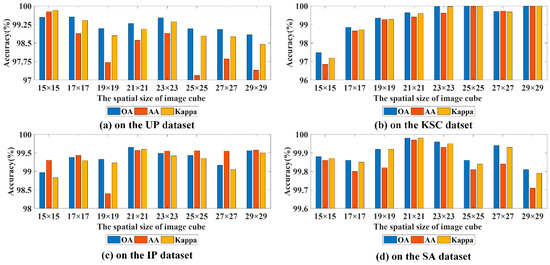
Figure 5. Three evaluation indexes for different spatial sizes on four experimental datasets.

3.2.2. Influence of Diverse Training Percentage

1%, 3%, 5%, 7%, 10%, 15%, 20%, 25% and 30% of samples are chosen at random as the training set and the corresponding remaining samples for test, which studies the influences of different numbers of training samples on the performance of our proposed method. The corresponding results of different training sample numbers for UP dataset, KSC dataset, IP dataset and SA dataset are provided in Figure 6. From Figure 6, we can clearly see that three evaluation indexes of four experimental datasets are gradually improved as the number of training samples increases. Concretely, for KSC dataset, as the number of training samples is 1%~7%, for IP dataset, as the number of training samples is 1%~10%, and for UP and SA datasets, as the number of training samples is 1% or 3%, it can be seen that three evaluation indicators of our proposed method are not so useful. As the number of training samples is more than 3% for UP dataset and SA dataset, all evaluation indicators are over 99%. For KSC dataset, as the number of training samples is more than 7%, and for IP dataset, as the number of training samples is more than 10%, all evaluation indicators exceed 99%. On the one hand, when the proportion of training samples is too small, because of the random choice of samples, some training samples are not selected, resulting in poor classification performance. As the proportion of training samples increases, three evaluation indexes also become better. As the proportion of training samples is 15%, three evaluation indicators on four datasets are over 99%. On the other hand, the KSC dataset and IP dataset have relatively few labeled samples, hence the classification results of the two datasets are relatively affected by the number of training samples. By contrast, the UP dataset and SA dataset include a mass of training samples, so it can still achieve good classification results without a large number of training samples. Therefore, for UP dataset and SA dataset, we randomly choose 10% of samples as the training set and the corresponding remaining 90% of samples are adopted as the test set. For KSC dataset and IP dataset, 20% of samples are selected at random for training and the corresponding remaining 80% of samples for testing.

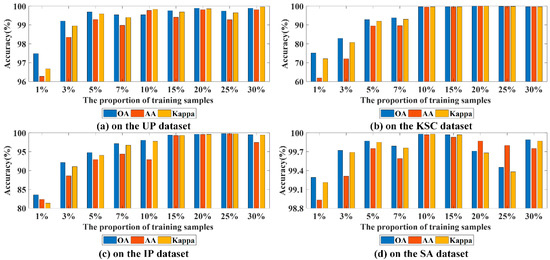
Figure 6. Three evaluation indexes for diverse training percentages on four experimental datasets.

3.2.3. Influence of Different Numbers of Principal Components

To reduce the computational cost and learning parameters, we apply PCA transformation to our proposed method. Different numbers of principal components (PCs) are set, i.e., {3, 5, 10, 15, 20, 25, 30, 35, 40}, to analyze the effect of it in our proposed method for different datasets. From Figure 7a, for UP dataset, compared with other conditions, as the number of PCs is 15, though OA is not good, AA and Kappa are obviously superior to others and three evaluation indicators are over 99.5%. Therefore, we set the number of PCs to 15 for UP dataset. From Figure 7b, for KSC dataset, as the number of PCs is 30 or 35, three evaluation indications reach 100%. Considering learning parameters and training time, we set the number of PCs to 30 for KSC dataset. From Figure 7c, as the number of PCs is 40, the IP dataset obtains the best classification accuracy. From Figure 7d, as the number of PCs is 30, the SA dataset achieves the optimal evaluation indicators, which are closer to 100%. Therefore, the number of PCs for IP dataset and SA dataset is set at 40 and 30, respectively.

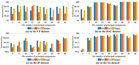
Figure 7. Three evaluation indexes for different numbers of PC on four experimental datasets.

3.2.4. Influence of Diverse Compressed Ratios in the DB

To explore the compressed ratios of the channel-wise recalibrate branch in the DB, the compressed ratios $r$ = 1, 2, 3, 4, 5 and 6 are utilized in the UP dataset, KSC dataset, IP dataset and SA dataset. Figure 8 shows the influences of diverse compressed ratios on four experimental datasets. From Figure 8a,b, as the compressed ratio of DB is 1, the UP dataset and KSC dataset obtain the optimal classification accuracy. Meanwhile, we find that large $r$ slightly degrades the evaluation indications, which means that it underfits the feature channel-wise correlations. As show in Figure 8c, as the compressed ratio of DB is 4, the IP dataset has the best evaluation indications. From Figure 8d, for SA dataset, as the compressed ratio of DB is 6, the OA, AA and Kappa are closer to 100%. By contrast, for IP dataset and SA dataset, the evaluation indications do not increase monotonically as $r$ decreases. A possible reason is that the channel attention branch in the DB overfits the feature channel-wise correlations. Therefore, the most appropriate compressed ratio of DB is 1, 1, 4 and 6 for UP dataset, KSC dataset, IP dataset and SA dataset, respectively.

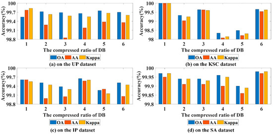
Figure 8. Three evaluation indexes for diverse compressed ratios in the DB on four experimental datasets.

3.2.5. Influence of Various Numbers of SFEBs

The SFEB can capture abundant high-frequency spectral-spatial features at different scales as well as take full advantage of features from the previous layers. Too small a number of SFEBs may insufficiently extract spectral-spatial features, while too large a number will increase computational cost. Therefore, it is indispensable to set the appropriate number of SFEBs to capture the multiscale spectral-spatial features. Figure 9 provides three evaluation indexes when the number of SFEBs is 1, 2, 3, 4, 5, 6, 7, 8, 9, 10, 11 and 12 on four experimental datasets. From Figure 9b, for KSC dataset, we can clearly see that, as the number of SFEBs is 2, 4, 5 and 6, three evaluation indexes reach 100% and achieve the first-rank classification performance. Compared with other conditions, when the number of SFEBs is 2, fewer learning parameters and shorter training time are needed. Therefore, the most appropriate number of SFEBs is 2 for KSC dataset. According to Figure 9a,c,d, we can obviously find that, when the number of SFEBs is 8, the UP dataset has excellent classification results; when the number of SFEBs is 9, three evaluation indexes of IP dataset achievemthe optimal accuracy; when the number of SFEBs is 2, the SA obtains-optimal classification accuracy. Therefore, we set the proper number of SFEBs as 8, 9 and 2 for UP dataset, IP dataset and SA dataset, respectively.

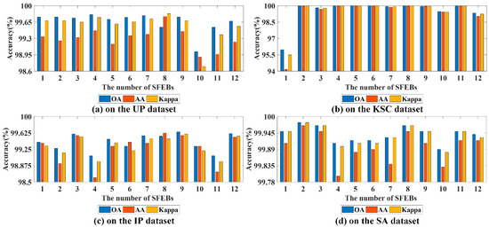
Figure 9. Three evaluation indexes for various numbers of SFEBs on four experimental datasets.

3.3. Comparisons with the State-of-the-Art Method

In this paper, several classical and advanced classification methods are compared to evaluate the performance of our proposed HS²FNet on four well-known datasets. Particularly, we divide these related classification methods into two categories: classification methods based on ML and classification methods based on DL. One includes three traditional classification methods: Support Vector Machine (SVM), Random Forest (RF), Multinomial Logistic Regression (MLR). The other includes nine representative classification methods utilizing DL, i.e., Deep Convolutional Neural Networks (1D_CNN) [29], Deep Learning Classifier (2D_CNN) [65], 3-D Deep Learning Approach (3D_CNN) [66], Exploring Feature Hierarchy based on 2D-3D-CNN (HybridSN) [67], Deep Multi-layer Fusion Dense Network (MFDN) [33], Spectral-Spatial Attention Network (SSAN) [44], Joint Spatial-Spectral Attention Network (JSSAN) [68], Dual-Channel Residual Network (DCRN) [69] and Multi-attention Fusion Network (MAFN) [70].

To obtain fair and impartial results, all classification methods including 12 compared methods and our proposed HS²FNet utilize the same number of training samples: 10%, 20%, 20% and 10% for UP dataset, KSC dataset, IP dataset and SA dataset, respectively. Table 5, Table 6, Table 7 and Table 8 report class-wise accuracy, OA, AA, and Kappa for four experimental datasets. Moreover, Figure 10, Figure 11, Figure 12 and Figure 13 display the visual maps of diverse classification methods. By comparing our presented HS²FNet with twelve classification methods, we can obtain the following conclusions.

Table 5. Quantitative comparisons of the state-of-the-art models and our network on UP dataset.

No.	SVM	RF	MLR	1D_CNN	2D_CNN	3D_CNN	HybridSN	MFDN	SSAN	JSSAN	DCRN	MAFN	HS2FNet
1	82.51	61.02	51.83	91.43	94.54	92.97	96.99	95.56	99.40	99.14	97.74	99.38	99.80
2	6.09	70.21	69.97	97.60	99.94	99.31	99.83	98.15	99.82	99.80	99.67	99.04	99.98
3	53.39	0.00	0.00	96.15	97.89	92.73	99.79	100.00	99.68	100.00	95.21	73.08	99.95
4	84.41	95.21	98.59	94.05	97.14	99.46	97.99	99.46	99.78	94.99	98.37	99.88	99.24
5	100.00	0.00	100.00	97.03	99.26	99.83	97.55	99.59	100.00	95.80	86.23	99.92	99.42
6	46.01	67.55	68.8	96.68	99.89	100.00	99.12	100.00	99.98	97.97	99.98	98.93	100.00
7	59.87	0.00	0.00	93.25	98.92	99.09	94.12	100.00	97.08	61.04	94.33	92.39	99.75
8	65.22	55.57	45.55	90.16	87.98	99.96	93.96	99.91	98.33	91.90	97.81	95.75	99.52
9	100.00	0.00	0.00	89.73	83.60	100.00	97.55	99.53	100.00	90.33	99.79	100.00	99.76
OA	62.96	67.50	66.41	95.30	97.24	98.07	98.35	98.88	99.56	96.13	98.26	97.00	99.83
AA	41.33	34.26	39.88	91.71	94.24	96.85	96.07	98.80	98.78	94.83	93.93	93.27	99.54
Kappa	45.12	52.43	50.45	93.74	96.35	97.43	97.81	98.51	99.41	94.89	97.69	96.02	99.77

The best accuracy of three evaluation indexes is marked in red. The highest category accuracy of the designed model is highlighted in blue.

Table 6. Quantitative comparisons of the state-of-the-art models and our network on KSC dataset.

No.	SVM	RF	MLR	1D_CNN	2D_CNN	3D_CNN	HybridSN	MFDN	SSAN	JSSAN	DCRN	MAFN	HS2FNet
1	44.31	45.39	39.10	89.22	97.81	100.00	100.00	100.00	100.00	95.88	100.00	100.00	100.00
2	92.56	71.74	0.00	48.56	93.60	98.40	98.35	98.98	100.00	98.78	30.93	98.45	100.00
3	65.19	0.00	0.00	74.56	93.00	67.00	97.06	94.86	98.07	95.34	0.00	100.00	100.00
4	52.27	0.00	0.00	23.40	84.09	98.04	98.45	97.91	100.00	93.51	100.00	96.09	100.00
5	61.25	0.00	0.00	64.84	97.60	97.62	96.97	99.22	100.00	88.65	0.00	98.41	100.00
6	46.90	0.00	0.00	75.84	97.53	100.00	98.35	100.00	100.00	99.44	34.31	66.17	100.00
7	66.67	0.00	0.00	0.00	91.03	83.17	100.00	100.00	100.00	100.00	5.29	74.34	100.00
8	86.30	78.72	49.64	65.59	97.69	51.50	99.12	99.42	99.71	95.77	0.00	99.42	100.00
9	92.79	72.64	54.59	62.73	97.15	100.00	99.05	99.05	99.52	95.58	0.00	100.00	100.00
10	100.00	100.00	91.75	77.50	96.40	99.38	99.07	100.00	99.69	96.34	100.00	100.00	100.00
11	100.00	96.25	70.10	74.92	95.07	100.00	98.53	100.00	99.70	99.09	100.00	100.00	100.00
12	97.82	83.81	100.00	49.91	92.92	98.52	95.26	100.00	96.40	99.75	88.01	98.53	100.00
13	100.00	89.37	99.54	90.16	99.87	99.87	99.73	100.00	100.00	98.54	100.00	100.00	100.00
OA	75.25	72.64	61.56	70.69	95.99	88.97	98.65	99.42	99.42	96.95	47.15	96.69	100.00
AA	61.41	53.58	42.38	61.93	93.85	91.41	98.18	99.00	99.12	95.30	46.82	94.99	100.00
Kappa	71.90	68.80	56.09	67.28	95.53	89.78	98.50	99.36	99.36	96.60	43.32	96.31	100.00

The best accuracy of three evaluation indexes is marked in red. The highest category accuracy of the designed model is highlighted in blue.

Table 7. Quantitative comparisons of the state-of-the-art models and our network on IP dataset.

No.	SVM	RF	MLR	1D_CNN	2D_CNN	3D_CNN	HybridSN	MFDN	SSAN	JSSAN	DCRN	MAFN	HS2FNet
1	92.31	100.00	57.14	100.00	87.50	97.06	100.00	100.00	100.00	100.00	66.67	100.00	97.30
2	64.25	63.13	61.06	86.86	100.00	89.04	94.11	99.29	99.82	82.73	99.18	98.46	99.74
3	67.11	68.09	65.84	93.14	96.74	100.00	98.77	100.00	99.85	100.00	98.91	97.22	99.85
4	52.50	55.00	45.70	100.00	80.62	99.45	98.37	97.79	99.47	98.30	95.34	89.78	100.00
5	84.63	86.67	67.27	97.10	94.06	89.35	97.18	100.00	98.47	92.77	91.02	100.00	100.00
6	90.58	89.44	87.30	98.27	99.31	95.09	100.00	99.66	100.00	100.00	89.55	98.15	100.00
7	85.71	90.00	89.47	100.00	100.00	100.00	100.00	100.00	100.00	100.00	100.00	100.00	100.00
8	95.14	88.22	91.39	100.00	100.00	98.71	99.74	100.00	100.00	97.45	92.27	94.09	100.00
9	28.57	0.00	0.00	100.00	100.00	100.00	100.00	100.00	100.00	100.00	72.22	100.00	100.00
10	71.99	71.21	65.93	95.88	94.07	100.00	96.33	99.59	99.87	94.90	99.15	96.75	100.00
11	69.86	72.01	63.44	93.98	97.04	99.84	97.78	97.85	98.39	98.68	95.30	98.49	99.49
12	67.05	54.93	47.94	88.49	94.73	94.14	96.11	92.73	99.16	90.87	96.01	85.71	99.37
13	90.45	91.41	92.86	100.00	97.62	100.00	9591	97.04	100.00	97.04	100.00	97.62	100.00
14	86.16	84.26	86.82	98.61	98.34	99.02	100.00	99.41	100.00	99.80	99.16	99.51	99.80
15	71.36	66.53	68.80	89.17	94.95	88.00	99.66	98.09	96.54	94.12	100.00	99.35	98.40
16	100.00	100.00	95.53	95.59	92.11	100.00	100.00	86.05	96.10	93.15	50.00	100.00	94.74
OA	74.67	73.92	70.04	94.07	96.66	96.27	97.66	98.46	99.26	94.85	95.31	97.17	99.65
AA	69.18	61.06	62.13	86.67	93.95	93.19	96.33	98.69	98.82	91.59	95.24	92.80	99.57
Kappa	70.86	70.16	65.41	93.22	96.19	95.75	97.33	98.25	99.15	94.13	94.66	96.77	99.60

The best accuracy of three evaluation indexes is marked in red. The highest category accuracy of the designed model is highlighted in blue.

Table 8. Quantitative comparisons of the state-of-the-art models and our network on SA dataset.

No.	SVM	RF	MLR	1D_CNN	2D_CNN	3D_CNN	HybridSN	MFDN	SSAN	JSSAN	DCRN	MAFN	HS2FNet
1	100.00	92.48	0.00	95.81	100.00	100.00	99.83	100.00	99.94	99.50	100.00	100.00	100.00
2	99.73	98.01	64.66	92.80	100.00	100.00	100.00	100.00	64.42	99.88	100.00	100.00	100.00
3	78.28	56.51	83.35	100.00	100.00	100.00	100.00	97.96	87.55	98.67	100.00	73.93	100.00
4	99.78	97.86	100.00	93.47	96.81	100.00	99.92	100.00	72.42	99.35	100.00	99.76	99.52
5	96.43	60.66	51.92	88.26	99.50	99.75	99.05	99.75	98.42	99.21	95.98	99.96	99.83
6	100.00	100.00	99.97	99.55	99.28	99.97	99.94	100.00	87.42	99.92	99.97	100.00	100.00
7	100.00	99.65	64.53	100.00	100.00	99.88	100.00	100.00	100.00	99.84	100.00	100.00	100.00
8	30.39	41.40	59.21	98.60	98.08	83.38	99.91	100.00	94.69	99.49	100.00	100.00	100.00
9	99.40	90.16	54.31	100.00	100.00	100.00	100.00	100.00	100.00	99.61	100.00	100.00	100.00
10	92.85	0.00	54.87	99.62	96.98	99.86	100.00	98.14	100.00	99.59	99.53	97.27	100.00
11	99.25	0.00	0.00	100.00	98.05	100.00	100.00	98.92	95.01	100.00	100.00	100.00	100.00
12	98.82	0.00	0.00	99.83	98.27	100.00	100.00	99.77	100.00	98.97	94.55	96.98	100.00
13	100.00	0.00	0.00	99.74	97.47	99.371	95.04	100.00	82.20	100.00	86.95	99.88	100.00
14	100.00	0.00	0.00	70.37	100.00	86.55	100.00	100.00	99.47	70.60	100.00	100.00	100.00
15	50.72	0.00	0.01	82.93	98.95	100.00	100.00	98.10	99.95	99.82	84.53	99.27	100.00
16	100.00	0.00	0.00	97.77	100.00	99.88	100.00	100.00	100.00	100.00	100.00	99.82	100.00
OA	58.63	64.34	61.20	94.53	98.96	95.50	99.83	99.51	92.22	98.79	96.85	98.32	99.98
AA	47.82	49.53	42.15	92.51	98.89	96.91	99.77	99.38	89.46	96.44	96.90	98.78	99.97
Kappa	51.51	58.50	55.64	93.92	98.85	94.98	99.81	99.45	91.32	98.66	96.50	98.13	99.98

The best accuracy of three evaluation indexes is marked in red. The highest category accuracy of the designed model is highlighted in blue.

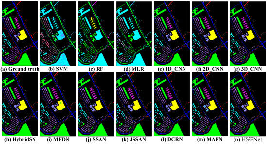
Figure 10. The visual comparisons of the state-of-the-art models and our network on UP dataset.

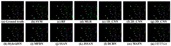
Figure 11. The visual comparisons of the state-of-the-art models and our network on KSC dataset.

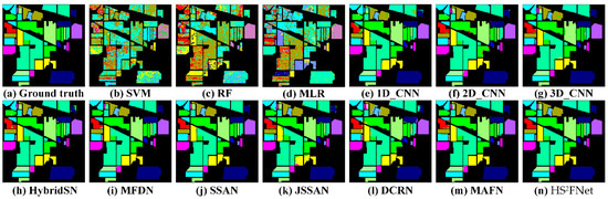
Figure 12. The visual comparisons of the state-of-the-art models and our network on IP dataset.

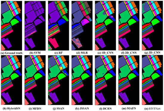
Figure 13. The visual comparisons of the state-of-the-art models and our network on SA dataset.

(1)

From Table 5, Table 6, Table 7 and Table 8, we can observe that, in comparison with three classification methods using ML, ten classification methods based on DL almost achieve superior classification results on four experimental datasets. Among them, our proposed HS2FNet occupies the first place. This is because ML-based methods all depend on hand-crafted features and prior knowledge, resulting in poor generalization performance, and cannot be well adapted to the classification task. By comparison, the DL-based classification methods can automatically extract hierarchical representations from HSI data. In addition, among ten DL-based classification methods, we also find that the classification accuracy of 1D_CNN is not satisfactory. This is because 1D_CNN only captures features in the spectral domain and ignores the rich spatial information of HSI.

(2)

The MFDN, SSAN, DCRN and MAFN adopt two CNN architectures to capture spectral features and spatial features, respectively. The simple concatenated operation or element-wise summation is utilized to fuse spectral and spatial features for classification. These methods obtain good classification results, but the close interdependency of spectral and spatial information is not excavated. Compared with them, our proposed method obtains the better classification accuracy on four datasets. For example, three evaluation indexes of our proposed HS²FNet are 99.98%, 99.97% and 99.98% on SA dataset, respectively, which are 3.14%, 3.07% and 3.48% higher than those of DCRN, and 0.47%, 0.49% and 0.53% higher than those of MFDN, respectively. Our proposed method uses the PFEM to capture multiscale spectral-spatial features while eliminating redundancy information, while the FRM is designed to mine second-order spectral-spatial statistic features to improve the classification performance.

(3)

The attention mechanism can capture key areas from images for classification. The SSAN introduces the self-attention mechanism, using the relationship between the pixels within an HSI cube to obtain attention areas. The JSSAN designs a spectral-spatial attention block to capture the long-range correlation of the spectral-spatial information. To eliminate redundant bands and interfering pixels, the MAFN constructs a band attention module and a spatial attention module. Although these attention mechanism-based classification methods can obtain evaluation indicators, they ignore the cross-dimension interaction. Comparec with these methods, our proposed method achieves the superior classification results on four datasets. For example, the designed model achieves 100% OA, 100% AA and 100% Kappa on KSC datasets, which are 0.58%, 0.88% and 0.64% higher than those of SSAN, 3.05%, 4.70% and 3.40% than those of JSSAN, and 3.31%, 5.01% and 3.69% than those of MAFN, respectively. Our designed DB not only pays more attention to adaptively recalibrating feature response to eliminate redundant features, but also learns close correlation of spatial and spectral data. Meanwhile, we utilize FCI, which heightens the representative ability of HSI by introducing cross-dimensional interaction without dimensionality reduction.

(4)

Figure 10, Figure 11, Figure 12 and Figure 13 illustrate the visual maps of 13 methods on UP dataset, KSC dataset, IP dataset and SA dataset, respectively. The visual results in these figures are consistent with the numerical values listed in Table 5, Table 6, Table 7 and Table 8. Compared with the ground-truth image, we can draw the conclusion that our proposed HS²FNet has smoother classification maps and higher classification accuracy. Meanwhile, it can make a better balance between the boundary information and the object continuity.

3.4. Generalization Performance

To further demonstrate the superiority and robustness of our devised network, we perform experiments among ten classification methods utilizing DL along with an increase in training samples, i.e., {1%, 3%, 5%, 7%,10%}. From Figure 14, we can see that our proposed method occupies the first place in all these cases on four experimental datasets, while other compared methods do not show good robustness and generalization performance. For example, according to Figure 14a, our presented HS²FNet achieves the top classification accuracy and the MAFN obtains the lowest accuracy. As the number of training samples is 1%, the OA of our proposed model is 97.48%, which is 52.44% higher than MAFN. In Figure 14b, HybridSN achieves comparable results among these classification methods. As the number of training samples is 7%, the OA of our proposed method is 93.80%, which is 3.14% higher than HybridSN. As exhibited in Figure 14c, the OA of 3D_CNN is worst in almost all cases. As the number of training samples is 10%, the OA of our proposed method is 98.04%, which is 18.87% higher than 3D_CNN.In Figure 14d, JSSAN ranks second among competition methods. As the number of training samples is 3%, the OA of our proposed method is 99.72%, which is 6.87%higher than JSSAN. Compared with these representative classification methods, the aforesaid experimental results adequately prove that our constructed HS²FNet possesses more robust generalization performance.

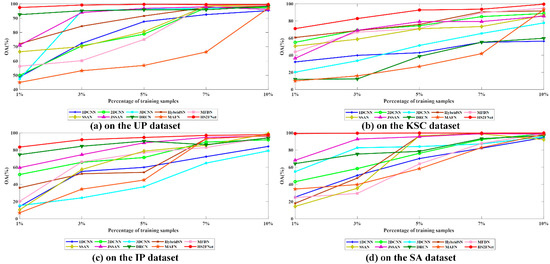
Figure 14. OA of various approaches with diverse numbers of training samples on four experimental.

3.5. Ablation Studies

3.5.1. Effectiveness Analysis of the SFEB

In this paper, we design the SFEB to make full use of spectral-spatial features at different scales and from the previous layers, which is an important component of our proposed HS²FNet.

The SFEB is composed of a symmetrical multiscale dense link unit, cross transmission and local skip transmission. To verify the advantages of the novel design in the proposed method, ablation experiments are conducted under six different conditions on four common datasets, labeled case 1, case 2, case 3, case 4, case 5 and case 6, respectively. The ablation results of module validity analysis are shown Table 9.

Table 9. Classification results of the SFEB with different building blocks on four public datasets.

Datasets	Indexes	Top	Bottom	Dense	Cross	Skip	OA	AA	Kappa
	Schemes
UP	Case 1	√		√			96.21	92.00	94.96
	Case 2		√	√			96.65	93.59	95.56
	Case 3	√	√				95.51	90.98	94.02
	Case 4	√	√	√			98.30	96.27	97.75
	Case 5	√	√	√	√		98.36	96.47	97.82
	Case 6	√	√	√	√	√	99.54	99.77	99.83
KSC	Case 1	√		√			85.76	75.71	84.05
	Case 2		√	√			93.27	90.49	92.50
	Case 3	√	√				94.76	91.87	94.16
	Case 4	√	√	√			95.08	92.93	94.51
	Case 5	√	√	√	√		97.50	96.74	97.22
	Case 6	√	√	√	√	√	100	100	100
IP	Case 1	√		√			96.94	88.22	96.51
	Case 2		√	√			97.13	86.79	96.74
	Case 3	√	√				96.12	85.04	95.57
	Case 4	√	√	√			97.67	90.96	97.34
	Case 5	√	√	√	√		97.97	95.26	97.69
	Case 6	√	√	√	√	√	99.65	99.57	99.60
SA	Case 1	√		√			96.01	95.16	95.56
	Case 2		√	√			94.96	95.55	94.39
	Case 3	√	√				96.73	96.16	96.36
	Case 4	√	√	√			98.62	97.35	98.46
	Case 5	√	√	√	√		99.12	99.04	99.02
	Case 6	√	√	√	√	√	99.98	99.97	99.98

The best mechanic is highlighted in red.

Case 1: SFEB only uses Top-Link unit.

Case 2: SFEB only uses Bottom-Link unit.

Case 3: SFEB uses the combination of Top-Link unit and Bottom-Link unit (without dense connection).

Case 4: SFEB uses the combination of Top-Link unit and Bottom-Link unit.

Case 5: SFEB uses the combination of Top-Link unit, Bottom-Link unit and cross transmission.

Case 6 (our proposed method): SFEB uses the combination of Top-Link unit, Bottom-Link unit, cross transmission and local skip transmission.

In case 1 and case 2, we only introduce a one-path dense link unit: Top-Link unit or Bottom-Link unit. In case 3, we build a symmetrical multiscale dense link unit without dense connection. In case 4, the combination of Top-Link unit and Bottom-Link unit is utilized to conduct the dual-branch multiscale dense link unit. From Table 9, we can find that case 4 obtains better classification results on four experimental datasets. Particularly, compared with case 1 or case 2, case 4 utilizes a dual-branch multiscale dense link unit to capture multiscale spectral-spatial features. For example, case 4 achieves 98.30% OA, 96.27% AA and 97.75% Kappa on the UP dataset, which are 2.09%, 4.27% and 2.79% higher than case 1 and 1.65%, 2.68% and 2.19%, respectively. Compared with case 3, case 4 introduces the dense connection to take full use of spectral-spatial features from the previous layers. For example, case 4 achieves 95.08% OA, 92.93% AA and 94.51% Kappa on the KSC dataset, which are 0.32%, 1.06% and 0.35% higher than case 3. These experimental results demonstrate that our designed symmetrical multiscale dense link unit is effective.

In case 5, the cross transmission is introduced to achieve spectral-spatial feature exchange and fusion. Compared with case 4, case 5 obtains preferable classification accuracy. For example, case 5 achieves 97.97% OA, 95.26% AA and 97.69% Kappa on IP dataset, which are 0.3%, 4.3% and 0.35% higher than case 4. This is because that the cross transmission makes spectral-spatial features at different scales from the Top-Link unit and Bottom-Link unit to be transmitted to each other. These experimental results demonstrate that our introduced cross transmission is effective.

Local skip transmission can not only solve the degradation problem but also increase training speed, so we introduce it into case 6 (our proposed method). As provided in Table 9, compared with case 5, case 6 obtains superior classification results on four common experimental datasets. These experimental results demonstrate that local skip transmission is beneficial for our proposed method.

3.5.2. Effectiveness Analysis of the DB

To fully verify the effectiveness of our designed DB, three utilizing hierarchical feature compared methods and three ablation experiments are performed on four experimental datasets, which are shown in Figure 15, labeled h1, h2, h3, h4, h5, h6 and h7, respectively. The experimental results of module valid analysis are shown Table 10.

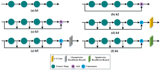
Figure 15. The structures of various fusion methods.

Table 10. Classification results of different fusion methods on four public datasets.

Datasets	Schemes	Case 1	Case 2	Case 3	Case 4	Case 5	Case 6	Case 7
	Indexes
UP	OA	97.42	97.86	97.79	97.89	97.89	98.39	99.54
	AA	93.70	95.18	95.33	95.60	95.60	96.32	99.77
	Kappa	96.57	97.16	97.07	97.19	97.19	97.87	99.83
KSC	OA	93.13	91.93	90.34	87.24	90.46	87.44	100
	AA	89.59	88.48	84.76	80.56	85.93	77.00	100
	Kappa	92.32	90.97	89.19	85.71	89.33	85.87	100
IP	OA	96.35	96.50	97.00	95.29	97.22	98.07	99.65
	AA	83.80	84.57	84.36	78.99	90.95	93.60	99.57
	Kappa	95.84	96.00	96.89	94.63	96.83	97.80	99.60
SA	OA	96.44	95.88	96.40	94.64	96.11	96.57	99.98
	AA	97.14	95.62	96.72	93.07	96.22	95.24	99.97
	Kappa	96.04	95.42	96.00	94.03	95.67	96.18	99.98

The best mechanic is highlighted in red.

h1: not using hierarchical features (as shown in Figure 15a).

h2: one residual connection only using input features (as shown in Figure 15b).

h3: residual dense connection using all hierarchical features (as shown in Figure 15c).

h4: using concatenated operation and $1\times 1$ convolutional layer for hierarchical feature fusion (as shown in Figure 15d).

h5: HFFB only using channel-wise recalibrate branch. (as shown in Figure 15e).

h6: HFFB only using spatial-wise recalibrate branch (as shown in Figure 15f).

h7: our proposed DB.

From Table 10, we can clearly see that h7 achieves the best classification results on four experimental datasets. On the one hand, compared with h1, h2 and h3, our proposed DB has obvious advantages. For example, h7 achieves 100% OA, 100% AA and 100% Kappa on the KSC dataset, which are 6.87%, 10.41% and 7.68% higher than h1. This is because DB can utilize two $1\times 1$ convolutional layers to reduce the number of feature maps without losing fine information, while focusing on adaptively recalibrating channel-wise and spatial-wise feature responses to achieve first-order spectral-spatial feature distillation.

On the other hand, compared with h4, h5 and h6, our proposed DB obtains better classification accuracy. For example, h7 obtains 99.98% OA, 99.97% AA and 99.98% Kappa on SA dataset, which are 3.41%, 4.73% and 3.8% higher than h6. Our designed DB can pay more attention to adaptively recalibrating feature responses to eliminate redundant features. Meanwhile, it also has ability to capture tight relation of spatial and spectral information. These experimental results demonstrate that our designed DB is effective.

3.5.3. Effectiveness Analysis of the Proposed HS²FNet

In this paper, we propose a HS²FNet for HIS classification, which is composed of three functional modules: SFEB, DB and FRM. To validate the effectiveness of each module in the proposed method, we execute the self-comparison experiments on four datasets under three conditions, labelling CN1, CN2 and CN3, respectively. The experimental results of module valid analysis are shown Table 11.

Table 11. Classification results of the proposed model with different building blocks on four public datasets.

Datasets	Schemes	CN1	CN2	CN3
	Indexes
UP	OA	95.98	96.27	99.54
	AA	93.80	94.21	99.77
	Kappa	94.65	95.04	99.83
KSC	OA	84.60	91.16	100
	AA	78.84	87.46	100
	Kappa	82.73	90.12	100
IP	OA	85.77	91.43	99.65
	AA	70.19	77.72	99.57
	Kappa	83.68	90.22	99.60
SA	OA	91.47	94.93	99.98
	AA	92.41	96.84	99.97
	Kappa	90.48	94.35	99.98

The best mechanic is highlighted in red. CN1: using the SFEB. CN2: using the SFEB and DB. CN3 (our proposed method): using the SFEB, DB and FRM.

From Table 11, we can clearly see that, compared with CN1, CN2 obtains better classification accuracy. CN2 introduces the DB to pay more attention to adaptively recalibrating feature response to eliminate redundant information. In particular, CN2 achieves 94.93% OA, 96.84% AA and 94.35% Kappa on SA dataset, which are 3.46%, 4.43% and 3.87% higher than CN1. CN2 achieves 96.27% OA, 94.21% AA and 95.04% Kappa on UP dataset, which are 0.29%, 0.41% and 0.39% higher than CN1. These indicate that the DB is effective.

Moreover, three evaluation indications of CN3 are the best among three conditions on four common experimental datasets, which are all over 99%. These experimental results show that the FRM introduces cross-dimensional features and second-order statistical features into our proposed method to produce more luxuriant and expressive spectral-spatial features, which improves the classification performance.

4. Conclusions

In this paper, we propose a hybrid-order spectral-spatial feature network (HS2FNet) for HSI classification. The HS2FNet consists of two main parts: a precedent feature extraction module (PFEM) including several symmetrical feature extraction blocks (SFEBs) and a distillation block (DB) to capture first-order spectral-spatial features, and feature rethinking module (FRM) to model second-order spectral-spatial features. FRM can further refine first-order features obtained from the PFEM and improve the classification performance. First, a SFEB is designed to extract multiscale spectral-spatial features and make full use of HSI feature flows between different scales. Connecting all multiscale spectral-spatial features is helpful for HSI classification. Unfortunately, these hierarchical features may bring some noise and redundant information, which is harmful for classification accuracy. Therefore, a DB is constructed to focus on adaptively recalibrating channel-wise and spatial-wise feature responses to achieve first-order spectral-spatial feature distillation. Then, to enrich feature representations and improve the classification performance, we devise a FRM to model more discriminative second-order spectral-spatial features, which can not only heighten the representative ability of HSI by capturing the importance of features cross-dimensionally, but also learn more discriminative representations by exploiting the second-order statistics of HSI. Progressive two functional modules can obtain refined spectral-spatial features and achieve an accurate and efficient classification. Finally, we utilize two fully connected layers, two dropout layers and a soft-max layer to finish the classification task. Experimental results demonstrate that the proposed method can render competitive results in contrast with the state-of-the-art classification methods. In addition, the ablation experiments also demonstrate that the proposed architecture is reasonable to improve the classification performance. However, this method also could be improved. For example, as the depth of network increases, the computational complexity is also increased; it often needs numerous training parameters, and a longer training time. These could be future research directions to improve the proposed method.

References

- Landgrebe, D. Hyperspectral image data analysis. IEEE Signal Process. Mag. 2002, 19, 17–28. [Google Scholar] [CrossRef]
- Hang, D.; Yokoya, N.; Chanussot, J.; Zhu, X. CoSpace: Common subspace learning from hyperspectral-multispectral correspondences. IEEE Trans. Geosci. Remote Sens. 2019, 57, 4349–4359. [Google Scholar] [CrossRef] [Green Version]
- Naoto, Y.; Jonathan, C.; Karl, S. Potential of resolution-enhanced hyperspectral data for mineral mapping using simulated EnMAP and Sentinel-2 images. Remote Sens. 2016, 8, 172. [Google Scholar]
- Bioucas-Dias, J.M.; Plaza, A.; Camps-Valls, G.; Scheunders, P.; Nasrabadi, N.; Chanussot, J. Hyperspectral remote sensing data analysis and future challenges. IEEE Geosci. Remote Sens. Mag. 2013, 1, 6–36. [Google Scholar] [CrossRef] [Green Version]
- Zhang, L.; Zhang, L.; Tao, D.; Huang, X.; Du, B. Hyperspectral remote sensing image subpixel target detection based on supervised metric learning. IEEE Trans. Geosci. Remote Sens. 2014, 52, 4955–4965. [Google Scholar] [CrossRef]
- Ghamisi, P.; Mura, M.D.; Benediktsson, J.A. A survey on spectral spatial classification techniques based on attribute profiles. IEEE Trans. Geosci. Remote Sens. 2015, 53, 2335–2355. [Google Scholar] [CrossRef]
- Sun, B.; Kang, X.; Li, S.; Benediktsson, J.A. Random-Walker-based collaborative learning for hyperspectral image classification. IEEE Trans. Geosci. Remote Sens. 2017, 55, 212–222. [Google Scholar] [CrossRef]
- Wang, Z.; Du, B.; Shi, Q.; Tu, W. Domain adaptation with discriminative distribution and manifold embedding for hyperspectral image classification. IEEE Geosci. Remote Sens. Lett. 2019, 16, 1155–1159. [Google Scholar] [CrossRef]
- Gong, Z.; Zhong, P.; Yu, Y.; Hu, W.; Li, S. A CNN with multiscale convolution and diversified metric for hyperspectral image classification. IEEE Trans. Geosci. Remote Sens. 2019, 57, 3599–3618. [Google Scholar] [CrossRef]
- Safari, K.; Prasad, S.; Labate, D. A Multiscale Deep Learning Approach for High-Resolution Hyperspectral Image Classification. IEEE Geosci. Remote Sens. Lett. 2021, 18, 167–171. [Google Scholar] [CrossRef]
- Gan, Y.; Luo, F.; Liu, J.; Lei, B.; Zhang, T.; Liu, K. Feature Extraction Based Multi-Structure Manifold Embedding for Hyperspectral Remote Sensing Image Classification. IEEE Access 2017, 5, 25069–25080. [Google Scholar] [CrossRef]
- Sun, Z.; Wang, C.; Wang, H.; Li, J. Learn multiple-kernel SVMs domain adaptation in hyperspectral data. IEEE Geosci. Remote Sens. 2013, 10, 1224–1228. [Google Scholar]
- Li, J.; Bioucas-Dias, J.M.; Plaza, A. Spectral–spatial hyperspectral image segmentation using subspace multinomial logistic regression and Markov random fields. IEEE Trans. Geosci. Remote Sens. 2012, 50, 809–823. [Google Scholar] [CrossRef]
- Ham, J.; Chen, Y.; Crawford, M.M.; Ghosh, J. Investigation of the random forest framework for classification of hyperspectral data. IEEE Trans. Geosci. Remote Sens. 2005, 43, 492–501. [Google Scholar] [CrossRef] [Green Version]
- Yuan, Y.; Lin, J.; Wang, Q. Hyperspectral Image Classification via Multitask Joint Sparse Representation and Stepwise MRF Optimization. IEEE Trans. Cybern. 2016, 46, 2966–2977. [Google Scholar] [CrossRef] [PubMed]
- Melgani, F.; Bruzzone, L. Classification of hyperspectral remote sensing images with support vector machines. IEEE Trans. Geosci. Remote Sens. 2004, 42, 1778–1790. [Google Scholar] [CrossRef] [Green Version]
- Li, S.; Jia, X.; Zhang, B. Superpixel-based Markov random field for classification of hyperspectral images. In Proceedings of the 2013 IEEE International Geoscience and Remote Sensing Symposium IGARSS, Melbourne, Australia, 21–26 July 2013; pp. 3491–3494. [Google Scholar]
- Shen, L.; Jia, S. Three-dimensional Gabor wavelets for pixel-based hyperspectral imagery classification. IEEE Trans. Geosci. Remote Sens. 2011, 49, 5039–5046. [Google Scholar] [CrossRef]
- Li, W.; Chen, C.; Su, H.; Du, Q. Local binary patterns and extreme learning machine for hyperspectral imagery classification. IEEE Trans. Geosci. Remote Sens. 2015, 53, 3681–3693. [Google Scholar] [CrossRef]
- Lu, T.; Li, S.; Fang, L.; Jia, X.; Benediktsson, J.A. From subpixel to superpixel: A novel fusion framework for hyperspectral image classification. IEEE Trans. Geosci. Remote Sens. 2017, 55, 4398–4411. [Google Scholar] [CrossRef]
- Camps-Valls, G.; Bruzzone, L. Kernel-based methods for hyperspectral image classification. IEEE Trans. Geosci. Remote Sens. 2005, 43, 1351–1362. [Google Scholar] [CrossRef]
- Chen, Y.; Nasrabadi, N.M.; Tran, T.D. Classification for hyperspectral imagery based on sparse representation. In Proceedings of the 2010 2nd Workshop on Hyperspectral Image and Signal Processing: Evolution in Remote Sensing, Reykjavik, Iceland, 14–16 June 2010; pp. 1–4. [Google Scholar]
- He, L.; Li, J.; Liu, C.; Li, S. Recent advances on spectral-spatial hyperspectral image classification: An overview and new guidelines. IEEE Trans. Geosci. Remote Sens. 2018, 56, 1579–1597. [Google Scholar] [CrossRef]
- Paul, A.; Chaki, N. Band selection using spectral and spatial information in particle swarm optimization for hyperspectral image classification. Soft Comput. 2022, 26, 2819–2834. [Google Scholar] [CrossRef]
- Chen, Y.; Zhao, X.; Jia, X. Spectral–Spatial classification of hyperspectral data based on deep belief network. IEEE J. Sel. Topics Appl. Earth Observ. Remote Sens. 2015, 8, 2381–2392. [Google Scholar] [CrossRef]
- Schölkopf, B.; Platt, J.; Hofmann, T. Greedy layer-wise training of deep networks. Int. Conf. Neural Inf. Process. Syst. 2017, 19, 153–160. [Google Scholar]
- Mou, L.; Ghamisi, P.; Zhu, X. Deep recurrent neural networks for hyperspectral image classification. IEEE Trans. Geosci. Remote Sens. 2017, 55, 3639–3655. [Google Scholar] [CrossRef] [Green Version]
- Fukushima, K.; Miyake, S.; Ito, T. Neocognitron: A self-organizing neural network model for a mechanism of visual pattern recognition. IEEE Trans. Syst. 1970, 13, 826–834. [Google Scholar]
- Hu, W.; Huang, Y.; Wei, L.; Zhang, F.; Li, H. Deep convolutional neural networks for hyperspectral image classification. J. Sensors 2015, 2015, 258619. [Google Scholar] [CrossRef] [Green Version]
- Li, S.; Zhu, X.; Liu, Y.; Bao, J. Adaptive spatial-spectral feature learning for hyperspectral image classification. IEEE Access 2019, 7, 61534–61547. [Google Scholar] [CrossRef]
- Yang, J.; Zhao, Y.; Chan, J.C. Learning and Transferring Deep Joint Spectral–Spatial Features for Hyperspectral Classification. IEEE Trans. Geosci. Remote Sens. 2017, 55, 4729–4742. [Google Scholar] [CrossRef]
- Zhang, Z.; Liu, D.; Gao, D.; Shi, G. S3Net: Spectral–Spatial–Semantic Network for Hyperspectral Image Classification With the Multiway Attention Mechanism. IEEE Trans. Geosci. Remote Sens. 2021, 60, 5505317. [Google Scholar] [CrossRef]
- Li, Z.; Wang, T.; Li, W.; Du, Q.; Wang, C.; Liu, C.; Shi, X. Deep Multi-layer Fusion Dense Network for Hyperspectral Image Classification. IEEE J. Sel. Topics Appl. Earth Observ. Remote Sens. 2020, 13, 1258–1270. [Google Scholar] [CrossRef]
- Chen, Y.; Jiang, H.; Li, C.; Jia, X.; Ghamisi, P. Deep feature extraction and classification of hyperspectral images based on convolutional neural networks. IEEE Trans. Geosci. Remote Sens. 2016, 54, 6232–6251. [Google Scholar] [CrossRef] [Green Version]
- He, K.; Zhang, X.; Ren, S.; Sun, J. Deep residual learning for image recognition. In Proceedings of the IEEE Conference on Computer Vision and Pattern Recognition, Las Vegas, NV, USA, 26 June–1 July 2016; pp. 770–778. [Google Scholar]
- Huang, G.; Liu, Z.; Van Der Maaten, L.; Weinberger, K.Q. Densely connected convolutional networks. In Proceedings of the IEEE Conference on Computer Vision and Pattern Recognition, Honolulu, HI, USA, 21–26 July 2017; pp. 2261–2269. [Google Scholar]
- Meng, Z.; Jiao, L.; Liang, M.; Zhao, F. Hyperspectral Image Classification With Mixed Link Networks. IEEE J. Sel. Topics Appl. Earth Observ. Remote Sens. 2021, 14, 2494–2507. [Google Scholar] [CrossRef]
- Paoletti, M.E.; Haut, J.M.; Plaza, J.; Plaza, A. Deep&dense convolutional neural network for hyperspectral image classification. Remote Sens. 2018, 10, 1454. [Google Scholar]
- Li, H.; Wang, W.; Pan, L.; Li, W.; Du, Q.; Tao, R. Robust capsule network based on maximum correntropy criterion for hyperspectral image classification. IEEE J. Sel. Topics Appl. Earth Observ. Remote Sens. 2020, 13, 738–751. [Google Scholar] [CrossRef]
- Mei, Z.; Yin, Z.; Kong, X.; Wang, L.; Ren, H. Cascade Residual Capsule Network for Hyperspectral Image Classification. IEEE J. Sel. Topics Appl. Earth Observ. Remote Sens. 2022, 15, 3089–3106. [Google Scholar] [CrossRef]
- Yu, H.; Zhang, H.; Liu, Y.; Zheng, K.; Xu, Z.; Xiao, C. Dual-Channel Convolution Network With Image-Based Global Learning Framework for Hyperspectral Image Classification. IEEE Geosci. Remote Sens. Lett. 2022, 19, 6005705. [Google Scholar] [CrossRef]
- Bo, X.; Li, J.; Li, Y.; Song, R.; Xi, Y.; Shi, Y.; Qin, D. Multi-Direction Networks With Attentional Spectral Prior for Hyperspectral Image Classification. IEEE Trans. Geosci. Remote Sens. 2021, 60, 5500915. [Google Scholar]
- Feng, J.; Feng, X.; Chen, J.; Cao, X.; Zhang, X.; Jiao, L.; Yu, T. Generative Adversarial Networks Based on Collaborative Learning and Attention Mechanism for Hyperspectral Image Classification. Remote Sens. 2020, 12, 1149. [Google Scholar] [CrossRef] [Green Version]
- Sun, H.; Zheng, X.; Lu, X.; Wu, S. Spectral–Spatial Attention Network for Hyperspectral Image Classification. IEEE Trans. Geosci. Remote Sens. 2020, 58, 3232–3245. [Google Scholar] [CrossRef]
- Gu, J.; Jiao, L.; Liu, F.; Yang, S.; Wang, R.; Chen, P.; Cui, Y.; Xie, J.; Zhang, Y. Random subspace based ensemble sparse representation. Pattern Recognit. 2018, 74, 544–555. [Google Scholar] [CrossRef]
- Xiang, J.; Wei, C.; Wang, M.; Teng, L. End-to-End Multilevel Hybrid Attention Framework for Hyperspectral Image Classification. IEEE Geosci. Remote Sens. Lett. 2022, 19, 5511305. [Google Scholar] [CrossRef]
- Zhang, X.; Shang, S.; Tang, S.; Feng, J.; Jiao, L. Spectral Partitioning Residual Network With Spatial Attention Mechanism for Hyperspectral Image Classification. IEEE Trans. Geosci. Remote Sens. 2022, 60, 5507714. [Google Scholar] [CrossRef]
- Ge, Z.; Cao, G.; Zhang, Y.; Li, X.; Shi, H.; Fu, P. Adaptive Hash Attention and Lower Triangular Network for Hyperspectral Image Classification. IEEE Trans. Geosci. Remote Sens. 2022, 60, 5509119. [Google Scholar] [CrossRef]
- Wang, X.; Tan, K.; Du, P.; Pan, C.; Ding, J. A Unified Multiscale Learning Framework for Hyperspectral Image Classification. IEEE Trans. Geosci. Remote Sens. 2022, 60, 4508319. [Google Scholar] [CrossRef]
- Yang, K.; Sun, H.; Zou, C.; Lu, X. Cross-Attention Spectral–Spatial Network for Hyperspectral Image Classification. IEEE Trans. Geosci. Remote Sens. 2022, 60, 5518714. [Google Scholar] [CrossRef]
- Lin, T.-Y.; RoyChowdhury, A.; Maji, S. Bilinear CNN models for fine-grained visual recognition. In Proceedings of the IEEE International Conference on Computer Vision, Santiago, Chile, 7–13 December 2015; pp. 1449–1457. [Google Scholar]
- Li, Y.; Wang, N.; Liu, J.; Hou, X. Factorized bilinear models for image recognition. In Proceedings of the IEEE International Conference on Computer Vision, Venice, Italy, 22–29 October 2017; pp. 2098–2106. [Google Scholar]
- Wang, Y.; Xie, L.; Liu, C.; Qiao, S.; Zhang, Y.; Zhang, W.; Tian, Q.; Yuille, A. SORT: Second-order response transform for visual recognition. In Proceedings of the IEEE International Conference on Computer Vision, Venice, Italy, 22–29 October 2017; pp. 1368–1377. [Google Scholar]
- He, N.; Paoletti, M.E.; Haut, J.M.; Fang, L.; Li, S.; Plaza, A.; Plaza, J. Feature extraction with multiscale covariance maps for hyperspectral image classification. IEEE Trans. Geosci. Remote Sens. 2019, 57, 755–769. [Google Scholar] [CrossRef]
- Zheng, J.; Feng, Y.; Bai, C.; Zhang, J. Hyperspectral image classify-cation using mixed convolutions and covariance pooling. IEEE Trans. Geosci. Remote Sens. 2020, 59, 522–534. [Google Scholar] [CrossRef]
- Gao, Z.; Xie, J.; Wang, Q.; Li, P. Global Second-order Pooling Convolutional Networks. In Proceedings of the 2020 IEEE/CVF Conference on Computer Vision and Pattern Recognition, Seattle, WA, USA, 13–19 June 2020; pp. 3019–3028. [Google Scholar]
- Zhang, C.; Li, G.; Du, S. Multi-Scale Dense Networks for Hyperspectral Remote Sensing Image Classification. IEEE Trans. Geosci. Remote Sens. 2019, 57, 9201–9222. [Google Scholar] [CrossRef]
- Fu, H.; Sun, G.; Ren, J.; Zhang, A.; Jia, X. Fusion of PCA and Segmented-PCA Domain Multiscale 2-D-SSA for Effective Spectral-Spatial Feature Extraction and Data Classification in Hyperspectral Imagery. IEEE Trans. Geosci. Remote Sens. 2022, 60, 5500214. [Google Scholar] [CrossRef]
- Hao, Q.; Sun, B.; Li, S.; Crawford, M.M.; Kang, X. Curvature Filters-Based Multiscale Feature Extraction for Hyperspectral Image Classification. IEEE Trans. Geosci. Remote Sens. 2022, 60, 5507916. [Google Scholar] [CrossRef]
- Cui, Y.; Zhou, F.; Wang, J.; Liu, X.; Lin, Y.; Belongie, S. Kernel pooling for convolutional neural networks. In Proceedings of the 2017 IEEE Conference on Computer Vision and Pattern Recognition, Honolulu, HI, USA, 21–26 July 2017; pp. 3049–3058. [Google Scholar]
- Li, P.; Xie, J.; Wang, Q.; Gao, Z. Towards faster training of global covariance pooling networks by iterative matrix square root normalization. In Proceedings of the 2018 IEEE/CVF Conference on Computer Vision and Pattern Recognition, Salt Lake City, UT, USA, 18–23 June 2018; pp. 947–955. [Google Scholar]
- Wang, H.; Wang, Q.; Gao, M.; Li, P.; Zuo, W. Multi-scale location-aware kernel representation for object detection. In Proceedings of the 2018 IEEE/CVF Conference on Computer Vision and Pattern Recognition, Salt Lake City, UT, USA, 18–23 June 2018; pp. 1248–1257. [Google Scholar]
- Hu, J.; Shen, L.; Sun, G. Squeeze-and-excitation networks. In Proceedings of the 2018 IEEE/CVF Conference on Computer Vision and Pattern Recognition, Salt Lake City, UT, USA, 18–23 June 2018; pp. 7132–7141. [Google Scholar]
- Huang, L.; Chen, Y. Dual-Path Siamese CNN for Hyperspectral Image Classification With Limited Training Samples. IEEE Geosci. Remote Sens. Lett. 2021, 18, 518–522. [Google Scholar] [CrossRef]
- Paoletti, M.E.; Haut, J.M.; Plaza, J.; Plaza, A. Deep learning classifiers for hyperspectral imaging: A review. ISPRS J. Photogramm. Remote Sens. 2019, 158, 279–317. [Google Scholar] [CrossRef]
- Hamida, A.B.; Benoit, A.; Lambert, P.; Amar, C.B. 3-D Deep Learning Approach for Remote Sensing Image Classification. IEEE Trans. Geosci. Remote Sens. 2018, 56, 4420–4434. [Google Scholar] [CrossRef] [Green Version]
- Roy, S.K.; Krishna, G.; Dubey, S.R.; Chaudhuri, B.B. HybridSN: Exploring 3-D–2-D CNN Feature Hierarchy for Hyperspectral Image Classification. IEEE Geosci. Remote Sens. Lett. 2020, 17, 277–281. [Google Scholar] [CrossRef] [Green Version]
- Li, J.; Yin, J.; Jia, X.; Li, S.; Han, B. Joint Spatial–Spectral Attention Network for Hyperspectral Image Classification. IEEE Geosci. Remote Sens. Lett. 2020, 18, 1816–1820. [Google Scholar] [CrossRef]
- Xu, Y.; Li, Z.; Li, W.; Du, Q.; Liu, C.; Fang, Z.; Zhai, L. Dual-Channel Residual Network for Hyperspectral Image Classification With Noisy Labels. IEEE Trans. Geosci. Remote Sens. 2022, 60, 5507916. [Google Scholar] [CrossRef]
- Li, Z.; Zhao, X.; Xu, Y.; Li, W.; Zhai, L.; Fang, Z.; Shi, X. Hyperspectral Image Classification With Multiattention Fusion Network. IEEE Geosci. Remote Sens. Lett. 2021, 19, 5503305. [Google Scholar] [CrossRef]
Publisher’s Note: MDPI stays neutral with regard to jurisdictional claims in published maps and institutional affiliations. |
© 2022 by the authors. Licensee MDPI, Basel, Switzerland. This article is an open access article distributed under the terms and conditions of the Creative Commons Attribution (CC BY) license (https://creativecommons.org/licenses/by/4.0/).