Multiple Spectral Resolution 3D Convolutional Neural Network for Hyperspectral Image Classification

Abstract

In recent years, benefiting from the rapid development of deep learning technology in the field of computer vision, the study of hyperspectral image (HSI) classification has also made great progress. However, compared with ordinary RGB images, HSIs are more like 3D cubes; therefore, it is necessary and beneficial to explore classification methods suitable for the very special data structure of HSIs. In this paper, we propose Multiple Spectral Resolution 3D Convolutional Neural Network (MSR-3DCNN) for HSI classification tasks. In MSR-3DCNN, we expand the idea of multi-scale feature fusion and dilated convolution from the spatial dimension to the spectral dimension, and combine 3D convolution and residual connection; therefore, it can better adapt to the 3D cubic form of hyperspectral data and make efficient use of spectral information in different bands. Experimental results on four benchmark datasets show the effectiveness of the proposed approach and its superiority as compared with some state-of-the-art (SOTA) HSI classification methods.

1. Introduction

Hyperspectral image (HSI) is a hot topic in remote sensing data analysis [1]. By combining rich spectral information with spatial information, HSI can support very accurate land use and land cover classifications for the ground surface, which is of great significance in agriculture [2], forestry [3], and other fields [4]. Land use and land cover classification tasks based on hyperspectral images are usually denoted as HSI classification. Rather than an ordinary image classification task, HSI classification is more similar to the semantic segmentation task in computer vision [5]. With the proposed model frameworks such as convolutional neural network (CNN) [6], the fully convolutional networks (FCN) [5], and residual network (ResNet) [7], deep learning technology has made great achievements in the field of RGB image processing. Deep learning technology has also been introduced to solve HSI classification tasks [4], such as the widely cited research work of Chen et al. [8] and Zhao et al. [9]. In recent years, more and more deep learning-based HSI classification approaches with different designs have been proposed, and huge improvements in classification accuracy have been reported [10,11,12,13,14].

However, as compared to the RGB images in a common semantic segmentation task, the structures of HSIs are much more complicated. For example, in the past, the Hyperion [15] sensor could provide 220 spectral bands, covering a spectrum range from 0.4 to 2.50 µm. At present, the more representative PRISMA [16] sensor can provide 240 spectral bands, covering a spectrum range from 0.4 to 2.45 µm. The newer Environmental Mapping and Analysis Program (EnMAP) [17] sensor provides 228 spectral bands, covering a spectrum range from 0.42 to 2.40 µm. It is clear that the number of channels in HSIs is relatively large relative to their spatial sizes, which makes HSI more like a three-dimensional cube of data. Therefore, some semantic segmentation methods designed for ordinary RGB images are no longer applicable to HSIs. Thus, the key to solving the classification problem of HSIs is to make efficient use of the rich spectral information in HSIs and to process 3D cubic data more efficiently. Inspired by the research work in [18], we use 3D convolution as the basis of the network to make the classification more suitable to the 3D structure of HSIs. As compared with the 2D convolutional kernel, the 3D convolutional kernel has one more dimension, which can extract spectral information more effectively.

Recently, we have noticed that models using multi-scale spatial features corresponding to different receptive fields can improve the semantic segmentation accuracy of ordinary RGB images. For example, PSPnet fuses features under four different scales and separates the feature map into different subregions forming pooled representation for different locations and size. Different levels of features are then concatenated as the final pyramid pooling global feature [19]. Similarly, the Inception Module uses different size convolution kernels to extract information at different levels, and the output feature maps are connected [20]. In our study, in order to enlarge the widths of the spectrums, we propose Spectral Dilated Convolutions (SDC) inspired by a Dilated Residual Network (DRN) [21]. At the same time, we extend this multi-scale feature fusion to the spectral dimension. Based on SDC and spectral multi-scale feature fusion, we propose a Multiple Spectral Resolution (MSR) module to extract the rich spectral information of HSIs. The module consists of multiple different 3D convolution branches corresponding to multiple different spectrum widths and can extract multi-scale spectral features of HSIs, respectively.

In the proposed network, we cascade two MSR modules as the essential component of the network. At the same time, in order to avoid the problem of gradient disappearance and gradient explosion, we refer to the idea of the residual network (ResNet) and add jump connection to the proposed network [7]. In general, we combine the above-mentioned MSR module, SDC, and 3D convolutional and residual connection to propose a Multiple Spectral Resolution 3D Convolutional Neural Network (MSR-3DCNN) for HSI classification. The main contributions of our work are summarized as follows:

(1)

For the cubic structure of HSI, we propose a fully 3D CNN HSI classification model.

(2)

Referring to the spatial Dilated Residual Network (DRN), we propose Spectral Dilated Convolutions (SDC). Referring to spectral multi-scale feature fusion, we propose spectral multi-scale feature fusion.

(3)

Based on SDC and spectral multi-scale feature fusion, we propose a Multiple Spectral Resolution (MSR) module. Combining the MSR module, SDC, and 3D convolution and residual connection, we propose Multiple Spectral Resolution 3D Convolutional Neural Network (MSR-3DCNN) for HSI classification.

(4)

Experimental results on four benchmark datasets show the effectiveness of MSR-3DCNN and its superiority as compared with some SOTA HSI classification methods.

The rest of the paper is organized as follows. Section 2 reviews the related work. Section 3 describes the proposed classification method. Section 4 introduces experimental settings and analyses the experimental results. Finally, conclusions and suggestions are provided in Section 5.

2. Related Work

In this section, we will introduce some basic knowledge and related work, including 3D convolutional neural network, multi-scale feature fusion, residual connection, and dilated convolution.

2.1. 3D Convolutional Neural Network

In a 2D CNN, convolution is applied to the two-dimensional feature graph, and the feature is calculated only from the spatial dimension. Formally, the value at position $(x,y)$ in the jth feature map in the ith layer, denoted as $v_{ij}^{xy}$, is given by

$$v_{ij}^{xy}=\Phi \left(b_{ij}+\sum _m\sum _{p=0}^{P_i-1}\sum _{q=0}^{Q_i-1}{w}_{ijm}^{pq}\times v_{(i-1)m}^{(x+p)(y+q)}\right)$$

(1)

where $\Phi$ is the activation function, $b_{ij}$ is the bias parameter for this feature map, m indexes over the set of feature maps in the $(i-1)$th layer connected to the current feature map, $w_{ijm}^{pq}$ is the weight parameter at the position $(p,q)$ of the kernel connected to the mth feature map, and $P_i$ and $Q_i$ are the height and width of the kernel, respectively.

In a 3D CNN, 3D convolution kernels [18] are applied to three-dimensional image cubes like HSIs, and the image features are calculated from both the spatial dimension and the spectral dimension simultaneously. Formally, the value at position $(x,y,z)$ on the jth feature map in the ith layer is given by

$$v_{ij}^{xyz}=\Phi \left(b_{ij}+\sum _m\sum _{p=0}^{P_i-1}\sum _{q=0}^{Q_i-1}\sum _{r=0}^{R_i-1}{w}_{ijm}^{pqr}\times v_{(i-1)m}^{(x+p)(y+q)(z+r)}\right)$$

(2)

where $R_i$ is the depth of the 3D convolutional kernel, $w_{ijm}^{pqr}$ is the weight parameter at the position $(p,q,r)$ of the kernel connected to the mth feature map in the previous layer, and the other parameters are the same as in the 2D convolutions. The parameters of CNN, such as the bias b and the kernel weight w, are usually trained using supervised approaches with the help of a gradient descent optimization technique [6,22]. 3D convolution is the base of some very powerful HSI classification models, such as hybrid spectral CNN (HybridSN) proposed by Roy et al. in [11] and Double-Branch Multi-Attention Mechanism Network (DBMA) proposed by Ma et al. in [12].

2.2. Multi-Scale Feature Fusion

Researchers have found that the fusion of multi-scale semantic features can improve the precision of semantic segmentation of common optical images. For example, in order to make use of spatial features corresponding to multiple scales, Zhao et al. proposed pyramid pooling module [19]. As illustrated in Figure 1, the pyramid pooling module integrates four levels of different pyramid scales. The first level gets a single value feature map through global pooling, and the next three levels get a feature map of different scales through pooling of different scales. A $\left(1\times 1\right)$ convolution is used after each feature map to reduce the channel of these feature maps. Then, bilinear interpolation is used to upsample these feature maps to the original spatial resolution of the input. Finally, all the feature maps are concatenated with the input of the module. The size of the final output is decided by the size of the input.

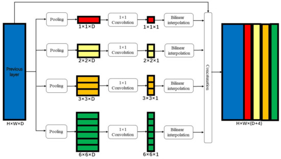
Figure 1. Structure of pyramid pooling module.

The Inception module [20] illustrated in Figure 2 can be considered as another implementation of this multi-scale spatial feature fusion idea. Convolution kernels of different sizes are used to extract spatial features corresponding to different scales, and the aggregation is also based on feature map concatenation.

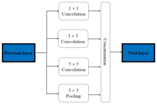
Figure 2. Structure of Inception module.

2.3. Residual Connections

The increase in model depth usually can improve the performance of a neural network model [23]. However, the increase in the depth of the model often causes the problem of gradient disappearance or gradient explosion. He et al. suggest that the residual connection solves this problem well [7] and greatly increases the depth of the networks. Therefore, at present, most convolutional neural networks use residual network (ResNet) as backbones.

As shown in Figure 3, the “shortcut connection” in a residual block is basically a direct connection between the input and the output of the block, while the “hidden block” usually contains several convolution layers along with batch normalization and activation.

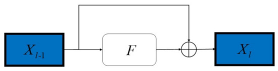
Figure 3. Structure of residual connection.

ResNet allows input information to pass directly and quickly to subsequent layers. The shortcut connections can be seen as identity mapping. In ResNet, the output of the l-th block be computed as

$$X_l=F\left(x_{l-1}\right)+h\left(x_{l-1}\right)$$

(3)

In general, through the residual connection, the original function can be divided into $F\left(x\right)$ and $h\left(x\right)$. $F\left(x\right)$ is almost the same as the original network. $h\left(x\right)$ can skip connections through shortcut connection.

2.4. Dilated Convolution

It is important to enlarge the receptive field of a segmentation model when we have to perform the classification and localization tasks simultaneously [24]. A direct way to obtain a large receptive field is to use large convolutional kernels; however, this means more model parameters and longer training time. An alternative is to use dilated convolutions [21], which can enlarge the receptive field without increasing the size of the model.

As shown in Figure 4, the red dot represents the convolution kernel and the blue base represents the receptive field. As shown in Figure 4a, it is a $\left(3\times 3\right)$ dilated convolution with the dilation rate set to 1, which is the same as a regular convolution. As shown in Figure 4b, it is a $\left(3\times 3\right)$ dilated convolution with the dilation rate set to 2. As shown in the red dots in the figure, the actual size of the convolution kernel is still $\left(3\times 3\right)$; however, the receptive field of the kernel is expanded to $\left(7\times 7\right)$. As shown in Figure 4c, when the dilation rate is set to 4, a $\left(3\times 3\right)$ dilated convolution kernel can hold a $\left(15\times 15\right)$ receptive field. Therefore, dilated convolution is helpful to expand the receptive field without increasing the number of parameters and original structure of the model.

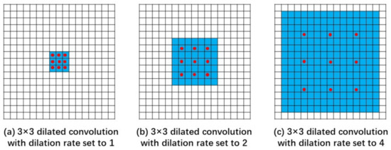
Figure 4. Schematic of dilated convolution.

3. The Proposed Approach

In this section, we illustrate in detail the proposed approach for HSI classification. First, we introduce Spectral Dilated Convolution (SDC). On the basis of SDC, we explain the Multiple Spectral Resolution (MSR) module which is an essential component of the proposed approach. Finally, we give a general illustration of Multiple Spectral Resolution 3D Convolutional Neural Network (MSR-3DCNN).

3.1. Spectral Dilated Convolutions

As described in Section 2.4, dilated convolution can expand the receptive field without changing the number of parameters and the original structure of the model. However, traditional 2D dilated convolutions can only be applied to enlarge the receptive field along spatial dimensions. Inspired by this, we propose the 3D spectral dilated convolution (SDC) to expand the receptive field of convolution kernels along the spectral dimension.

As shown in Figure 5, the black cuboids represent the convolution kernel and the red line cuboids cover the receptive field. As shown in Figure 5a, it is a $\left(3\times 3\times 3\right)$ spectral dilated convolution (SDC) with the spectral dilation rate (SDR) set to 1, which is the same as a regular 3D convolution kernel. As shown in Figure 5b, it is a $\left(3\times 3\times 3\right)$ SDC with the SDR set to 2 and the receptive field of the SDC kernel reaches $\left(3\times 3\times 7\right)$. As shown in Figure 5c, it is a $\left(3\times 3\times 3\right)$ SDC with the SDR set to 3. Without increase the size of the kernel, the receptive field is further enlarged to $\left(3\times 3\times 11\right)$. The receptive field of SDC is decided by the spectral dilation rate as

$$Rf=2\times SDR-1$$

(4)

$$K_{equ}=K_{real}+\left(K_{real}-1\right)\times \left(SDR-1\right)$$

(5)

$$R{F}_{i+1}=R{F}_i+\left(K_{equ}-1\right)\times S{P}_i$$

(6)

$$S{P}_i=\prod _{i=1}^{i}Strid{e}_i$$

(7)

where $Rf$ represents the receptive field of a single convolution kernel in spectral depth. $SDR$ represents the spectral dilation rate (SDR). $K_{equ}$ represents the number of the equivalent convolution kernels at spectral depth. $K_{real}$ represents the number of the real convolution kernels at spectral depth. $R{F}_{i+1}$ represents the receptive field of the current layer in spectral depth. $R{F}_i$ represents the receptive field of the previous layer in spectral depth. $S{P}_i$ represents the product of all the previous layers stride, and the current layer is not included. $Strid{e}_i$ represents the ith layer stride.

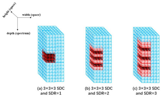
Figure 5. Schematic of spectral dilated convolution.

3.2. Multiple Spectral Resolution Module

Inspired by multi-scale feature fusion, we propose to construct a Multiple Spectral Resolution (MSR) module to make better usage of the rich spectral information in HSIs. As shown in Figure 6, the Multiple Spectral Resolution (MSR) module consists of multiple different convolution branches, and each branch consists of multiple SDCs. SDCs in the same branch are exactly the same, and all the SDCs share the same height (H) and width (W). In all the branches, the SDR values S1, S2 ... increase successively, so the SDC depths (D) of different branches are different.

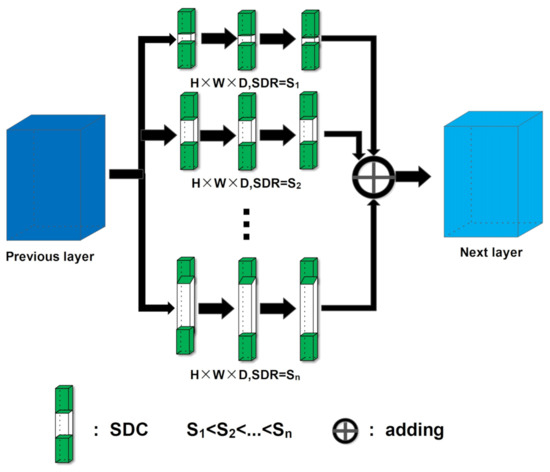
Figure 6. Structure of multiple spectral resolution module.

We keep the size of the output of each SDC the same as the input. The input passes through different branches, and then the output results of the branches are added. Finally, the sum is taken as the output of the MSR model. This design makes the branches have the same receptive field in the spatial dimension and different receptive field in spectral depth. If the parameters are set properly, the receptive fields of different branches in spectral depth can differ by many times. Therefore, multiple spectral resolution features can be extracted and fused by the proposed MSR model.

3.3. Multiple Spectral Resolution 3D Convolutional Neural Network

The MSR modules based on SDC in our proposed network can extract and fuse features corresponding to multiple spectral resolutions, and therefore the rich spectral information can be more effectively used. We also employ residual blocks to deepen the proposed model while avoid the vanishing gradient problem. Both the MSR module and the residual block are composed of 3D convolutions; therefore, we named the proposed model as Multiple Spectral Resolution 3D Convolutional Neural Network (MSR-3DCNN).

As shown in Figure 7, MSR-3DCNN consists of a set of individual SDCs, two MSR modules cascaded in the form of residual connection, two 3D Residual modules, and a set of fully connected layers. The first two layers of the model are composed of SDCs, with the same size of $\left(1\times 1\times 3\right)$ and the same dilation rate of 3. There are 32 SDC kernels in the first layer and 8 SDC kernels in the second one. Following the individual SDC layers are two identical MSR modules. Each MSR module consists of three types of SDCs, which share the same size as $\left(3\times 3\times 7\right)$, while their dilation rates are set to 1, 7, and 11, respectively. According to Equations (5)–(7), we calculate the receptive fields of the three branches in the spectral depth as 14, 129, and 216, respectively. The two 3D residual convolution blocks are quite similar. They share the same structure, with only some differences in the size of the 3D convolution kernels used in the main path of each block. At the end of both modules is a $\left(2\times 2\times 2\right)$ 3D pooling. Finally, there are two fully connected layers which contain 256 and 128 neurons, respectively. In order to avoid overfitting, we use Dropout [25] in the fully connected layers and add batch normalization [26] after them.

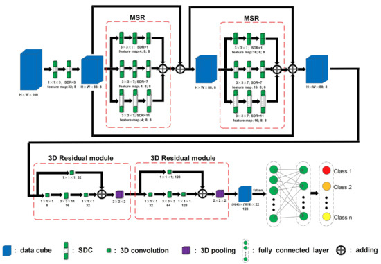
Figure 7. Schematic of Multiple Spectral Resolution 3D Convolutional Neural Network.

The model takes $\left(H\times W\times 100\right)$ image patches as inputs. A preprocessing based on principal component analysis (PCA) [27,28] is applied beforehand to reduce the original spectral dimensions of HSIs to 100. No padding is applied along the spectral dimension in the first two individual SDC layers; therefore, we get feature cubes with the size of $\left(H\times W\times 88;8\right)$. Then, in both the MSR modules, the size of the feature cubes is kept constant; therefore, skip connections can be used to directly connect the outputs and the inputs of these two modules. The data flow can be expressed as follows:

$$\begin{array}{cc}\hfill M_{second}& =f_{bra1}\left(M_{first}\right)+f_{bra2}\left(M_{first}\right)+f_{bra3}\left(M_{first}\right)+M_{first}\hfill \\ \hfill & =f_{MSR}\left(M_{first}\right)+M_{first}\hfill \end{array}$$

(8)

$$M_{third}=f_{MSR}\left(M_{second}\right)+M_{second}+M_{first}$$

(9)

where $M_{first}$ represents the input feature map of the first MSR. $M_{second}$ represents the output feature map of the first MSR. $M_{third}$ represents the output feature map of the second MSR. $f_{bra1},f_{bra2},$ and $f_{bra3}$ represent the arithmetic processing of three branch in MSR. $f_{MSR}$ represents the arithmetic processing of MSR. Through the second part of the network, two MSR modules and MSR-3DCNN achieve further spectral feature extraction and multiple spectral resolution fusion. Although same paddings are used in all the 3D convolution kernels in the two residual convolution blocks of the model, the size of the feature cubes are reduced to $\left(H/4\times W/4\times 22\right)$ by the 3D poolings at the end of each residual block. At last, these feature cubes are flattened and further processed by the fully connected layers.

The main idea of the proposed MSR-3DCNN is based on two novel designs: spectral dilated convolution and multiple spectral resolution fusion. Spectral dilated convolution is an extension of the classical dilated convolution from the spatial dimension to the spectral dimension, and the concept of multiple spectral resolution fusion is inspired by the spatial dimension technique, multi-scale fusion. These two designs give the proposed model three advantages: First of all, operations based on SDC are quite efficient to extract spectral features in HSIs. Then, the MSR modules in the proposed model can effectively make use of the rich spectral information in HSIs. As more attention has been paid to the processing of spectral information, MSR-3DCNN shows less reliance on spatial information and therefore is more robust to images with different spatial structures.

4. Experiments and Discussion

4.1. Datasets Description

In the experiments, four widely used HSI datasets are used to test the proposed approach: the Indian Pines (IP) dataset, the Salinas scene (SA) dataset, the Pavia University scene (PU) dataset, and the Botswana (BO) dataset. These datasets are quite complex some as there are many different land cover types in these scenes, such as corn, soybean, woods, fallow, stubble, celery, gravel, trees, occasional swamps, and many other types. Some of these land cover types are quite similar and difficult to distinguish. Furthermore, these data sets are obviously different from each other. The IP, SA, and BO data sets represent three different agriculture and forest areas, and the PU data set mainly consists of urban objects. These datasets are available and have been shared among researchers for years (These datasets can be found at http://www.ehu.eus/ccwintco/index.php/Hyperspectral_Remote_Sensing_Scenes.). Table 1 shows the summary of the characteristic of the datasets.

Table 1. Summary of the characteristics of the IP, SA, PU, and BO datasets.

Description	Datasets
	IP	SA	PU	BO
Sensor	AVIRIS	AVIRIS	ROSIS	Hyperion
Pixels	$145\times 145$	$512\times 217$	$610\times 340$	$1476\times 256$
GSD	20 m/pixel	3.7 m/pixel	1.3 m/pixel	30 m/pixel
Spectral range	0.4 to 2.5 µm	0.4 to 2.5 µm	0.43 to 0.86 µm	0.4 to 2.5 µm
Original band ${}^{\left(1\right)}$	224	224	103	242
Processed band ${}^{\left(2\right)}$	200	204	103	145
Ground truth ${}^{\left(3\right)}$	10,249	54,129	42,776	3248
Class ${}^{\left(4\right)}$	16	16	9	14
Mode	Airborne	Airborne	Airborne	Satellite

⁽¹⁾ number of spectral bands in the original HSI. ⁽²⁾ number of spectral subsetted from the raw dataset. ⁽³⁾ number of pixels for ground-truthing. ⁽⁴⁾ number of land cover and land use classes.

The Indian Pines (IP) dataset [29] was gathered by the airborne sensor, Airborne Visible Infrared Imaging Spectrometer (AVIRIS), from an agricultural and forest region, in the northwestern of India. The HSI consists of $\left(145\times 145\right)$ pixels with a ground sampling distance (GSD) of 20 m per pixel (m/pixel) and 224 spectral bands in the wavelength range 0.4 to 2.5 µm. The 24 water-absorbing spectral bands have been discarded, considering the remaining 200 bands for the experiments. The ground truth available is 10,249 pixels from a total of 21,025 and designated into 16 classes, e.g., corn, soybean, woods, etc.

The Salinas scene (SA) dataset [29] was also gathered by the AVIRIS sensor from an agricultural field of the Salinas Valley, California, USA. The HSI consists of $\left(512\times 217\right)$ pixels with a GSD of 3.7 m/pixel and 224 spectral bands in the wavelength range 0.4 to 2.5 µm. The 20 water-absorbing spectral bands have been discarded, considering the remaining 204 bands for the experiments. The ground truth available is 54,129 pixels from a total of 111,104 and designated into 16 classes, e.g., fallow, stubble, celery, etc.

The Pavia University scene (PU) dataset [30] was gathered by the Reflective Optics System Imaging Spectrometer (ROSIS) sensor on airborne vehicle from the urban area of Pavia University, in northern Italy. The HSI consists of $\left(610\times 340\right)$ pixels with a GSD of 1.3 m/pixel and 103 spectral bands in the wavelength range 0.43 to 0.86 µm. The ground truth available is 42,776 pixels from a total of 207,400 and designated into 9 classes, e.g., asphalt, gravel, trees, etc.

The Botswana (BO) dataset [31] was gathered by the Hyperion sensor on the Earth Observing One (EO-1) satellite from the vegetation and swamps, Okavango Delta, Botswana. The HSI consists of $\left(1476\times 256\right)$ pixels with a GSD of 30 m/pixel and 242 spectral bands in the wavelength range 0.4 to 2.5 µm. Uncalibrated and noisy bands that cover water absorption features were removed, considering the remaining 145 bands for the experiments. The ground truth available is 3248 pixels from a total of 377,856 and designated into 14 classes, e.g., seasonal swamps, occasional swamps, drier woodlands located, etc.

4.2. Experiment Settings

Figure 8 illustrates the whole framework of our Experiment. First, preprocessings, including principal component analysis (PCA) and cropping, are performed on the HSI dataset. PCA changes the spectral band from the original to 100. After the PCA process, $\left(N\times N\right)$ image patches are cropped from the dimension reduced HSI, and the ground truth label corresponding to the center pixel of each patch is assigned to the patch. Therefore, a set of labeled patches are obtained. Then, the labeled patches are randomly divided into two groups: the training set and test set. The training set is used to train network parameters and the test set is used to evaluate the effectiveness of the classification method.

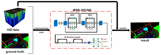
Figure 8. The training procedure of our method.

The proposed architecture is implemented using TensorFlow [32]. The hardware device is a server equipped with a NVIDIA GeForce RTX 3060 GPU and 32 GB of RAM. The source code can be found at github (https://github.com/shouhengx/MSR-3DCNN). Appendix A gives some brief descriptions about the environment in which the code runs and how it runs. During the training stage, the learning rate is initialized as 0.001 and the Adam algorithm is adopted to optimize the learning rate after each iteration. During the evaluation stage, three metrics, i.e., overall accuracy (OA) [33], average accuracy (AA) [34], and Kappa coefficient [34], are used to quantitatively evaluate the overall performance of the classification. OA refers to the ratio of the number of correct classifications to the total number of pixels to be classified. AA refers to the average accuracy of all classes. Kappa coefficients are used for consistency testing and can also be used to measure classification accuracy. In detail, the F1 score [35] is used to quantitatively evaluate the classification of each class. The F1 score combines the precision and recall metrics. At the same time, McNemar’s test [36] is conducted to analyze the statistical significance of the proposed method with the other methods. This test is based upon the standardized normal test statistic:

$$Z=\frac{f_{12}-f_{21}}{\sqrt{f_{12}+f_{21}}}$$

(10)

where $f_{12}$ indicates the number of samples classified correctly by classifier 1 and incorrectly by classifier 2. Similarly, $f_{21}$ indicates the number of samples classified correctly by classifier 2 and incorrectly by classifier 1. The difference in accuracy between classifiers 1 and 2 is said to be statistically significant if $\left|Z\right|>1.96$. The sign of Z indicates whether classifier 1 is more accurate than classifier 2 (Z > 0), and vice versa (Z < 0).

4.3. Comparisons with State-of-the-Art Methods

We preprocess the datasets through PCA and cropping as mentioned in Section 4.2. Then, using exactly the same testing protocol, we reproduce several HSI classification methods and compare them with the proposed method using $\left(9\times 9\right)$, $\left(11\times 11\right)$ and $\left(13\times 13\right)$ patch sizes, respectively. Ten percent of the labeled samples is used to train the models. In addition, we fuse the Predicted results of three independent classifiers under different patch sizes by sum rule [37]. The compared methods include contextual deep CNN [10], hybrid spectral CNN (HybridSN) [11], Double-Branch Multi-Attention mechanism network (DBMA) [12], and the most recent methods Fast 3D CNN [13] and Multi-scale Residual Network (MSRN) [14].

The overall accuracy results on the BO, IP, SA, and PU datasets are reported in Table 2. Figure 9 shows the overall accuracy changes of the BO, IP, SA, and PU datasets with 10% training samples and different patch sizes. Among the compared methods, the methods incorporating 3D convolution to extract spectral information, i.e., HybridSN, DBMA, Fast 3D CNN, MSRN, and MSR-3DCNN, have better OAs than the method using only 2D convolution, i.e., contextual deep CNN. Due to the fact that more attention is paid to the processing of spectral dimension information, MSR-3DCNN achieved good results on all experimental patch sizes, and this advantage is especially obvious in the case of small patch size. This indicates the robustness of MSR-3DCNN to the change of patch size. Furthermore, the proposed method performs well on all the four datasets, and its performance is especially good on the SA dataset. On the contrary, the spectral information processing takes a much less import role in the model of MSRN. This can be the reason for the unstable performances of MSRN on different data sets. For small data sets with uneven sample distribution (such as BO and IP), appropriate patch size is required for MSRN to perform well.

Table 2. Overall Accuracy (%) of the predictions by contextual deep CNN, HybridSN, DBMA, Fast 3D CNN, MSRN, and MSR-3DCNN using different patch size and the fuse the prediction results of these predictions obtained by sum rule.

Datasets	Patch Size	Models
		Contextual Deep CNN	HybridSN	DBMA	Fast 3D CNN	MSRN	MSR-3DCNN
BO	$9\times 9$	67.37	97.26	97.30	98.50	95.42	98.80
IP		60.65	96.41	98.03	97.04	95.83	98.10
SA		99.82	99.65	99.91	99.88	99.94	99.96
PU		97.60	99.28	99.58	99.37	99.84	99.62
BO	$11\times 11$	74.38	99.15	98.87	97.95	86.97	98.60
IP		64.23	97.39	98.60	97.47	91.14	97.56
SA		99.95	99.82	99.95	99.81	99.96	99.97
PU		97.60	99.00	99.64	99.60	99.85	99.60
BO	$13\times 13$	79.21	99.59	99.08	97.95	91.93	99.15
IP		72.44	97.77	97.08	98.51	97.21	97.30
SA		99.95	99.79	99.91	99.93	99.92	99.99
PU		98.38	99.60	99.54	99.19	99.84	99.72
BO	Fusion	85.94	99.08	99.97	99.45	91.21	99.62
IP		73.05	98.33	98.68	98.35	98.23	98.41
SA		99.97	99.93	99.95	99.91	99.97	99.98
PU		98.73	99.59	99.72	99.52	99.90	99.76

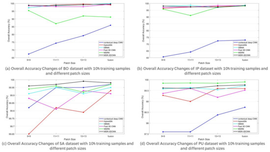
Figure 9. Changes of the overall accuracy of predictions on the four datasets, using 10% samples for training and different patch sizes.

Table 3, Table 4, Table 5 and Table 6 show the performance of the different classification methods using $\left(9\times 9\right)$ patch size and 10% of samples on different datasets in more details. Overall, MSR-3DCNN achieved good performance on different data sets using $\left(9\times 9\right)$ patch size. On the BO and the IP datasets, the best values for OA, AA, and Kappa Coefficient are all achieved by MSR-3DCNN. On the SA datasets, the OA and Kappa Coefficient of MSR-3DCNN are also the best and the AA is the second best result. On the PU dataset, the OA and Kappa Coefficient of MSR-3DCNN are the second best. At the same time, MSR-3DCNN shows better reliability on basically all the classes, and the advantage is quite obvious for some classes with very few samples for training such as Class 10 of BO dataset and Class 9 of IP dataset.

Table 3. F1 Score (%) for Each Class, OA (%), AA (%), and Kappa Coefficient Values for the entire dataset, training time (s), and test time (s) using $\left(9\times 9\right)$ patch size and 10% samples for training on the BO datasets.

Class	Training	Test	Models
Total	324	2924	Contextual Deep CNN	HybridSN	DBMA	Fast 3D CNN	MSRN	MSR-3DCNN
1	27	243	83.48	100.00	99.38	99.18	99.79	99.38
2	10	91	62.82	100.00	98.38	100.00	94.30	99.45
3	25	226	93.05	99.12	100.00	98.91	100.00	100.00
4	21	194	95.31	93.27	100.00	98.98	99.48	99.74
5	27	242	54.95	92.48	99.17	95.91	96.03	95.54
6	27	242	45.82	91.86	99.59	97.73	94.17	96.45
7	26	233	78.87	100.00	99.79	99.36	100.00	100.00
8	20	183	82.58	100.00	99.46	100.00	99.19	99.19
9	31	283	53.55	98.41	99.65	96.73	98.57	97.75
10	25	223	51.69	99.33	84.75	99.55	90.42	99.55
11	30	275	75.27	99.45	90.16	100.00	85.80	99.10
12	18	163	46.93	99.08	97.31	99.38	94.77	99.38
13	27	241	45.52	99.79	98.10	99.59	91.20	99.59
14	10	85	30.51	75.91	97.70	89.17	93.83	100.00
OA			67.37	97.26	97.30	98.50	95.42	98.80
AA			64.91	95.86	97.53	97.86	95.47	98.89
Kappa coefficient			0.6458	0.9703	0.9707	0.9837	0.9503	0.9870
Training time			19.35	17.66	50.02	14.28	51.86	224.18
Test time			0.74	0.73	1.99	0.48	1.54	7.09

Table 4. F1 Score (%) for each class OA (%), AA (%), and Kappa coefficient values for the entire dataset, training time (s), and test time (s) using $\left(9\times 9\right)$ patch size and 10% samples for training on the IP dataset.

Class	Training	Test	Models
Total	1024	9225	Contextual Deep CNN	HybridSN	DBMA	Fast 3D CNN	MSRN	MSR-3DCNN
1	5	41	22.64	100.00	80.00	100.00	42.31	89.19
2	143	1285	27.84	95.92	97.38	96.71	93.22	97.74
3	83	747	22.14	94.30	98.26	92.62	92.59	97.88
4	24	213	60.96	95.35	98.61	88.31	81.67	95.63
5	48	435	88.30	97.93	97.92	97.83	98.27	99.08
6	73	657	81.01	99.70	98.46	98.94	98.79	99.00
7	3	25	27.59	100.00	100.00	100.00	96.15	100.00
8	48	430	92.76	100.00	99.08	100.00	97.07	99.08
9	2	18	12.90	68.97	53.33	80.00	28.57	97.14
10	97	875	24.38	92.04	97.83	96.86	97.20	97.33
11	245	2210	71.90	96.22	97.88	97.58	97.13	98.43
12	59	534	30.79	93.79	97.13	95.26	94.47	96.16
13	20	185	80.00	100.00	99.73	99.73	99.73	98.93
14	126	1139	91.01	99.08	99.56	99.17	98.53	99.39
15	39	347	43.12	97.51	98.40	96.75	95.51	97.35
16	9	84	42.75	96.47	96.39	95.29	94.12	93.57
OA			60.65	96.41	98.03	97.04	95.83	98.10
AA			50.31	94.45	93.05	94.77	85.78	96.40
Kappa coefficient			0.5447	0.9591	0.9775	0.9663	0.9523	0.9784
Training time			39.09	33.45	126.40	30.99	117.89	667.04
Test time			1.51	1.33	5.23	1.02	3.80	19.30

Table 5. F1 Score (%) for each class, OA (%), AA (%), and Kappa Coefficient values for the entire dataset, training time (s), and test time (s) using $\left(9\times 9\right)$ patch size and 10% samples for training on the SA dataset.

Class	Training	Test	Models
Total	5412	48,717	Contextual Deep CNN	HybridSN	DBMA	Fast 3D CNN	MSRN	MSR-3DCNN
1	201	1808	99.75	100.00	100.00	100.00	100.00	100.00
2	372	3354	100.00	100.00	100.00	100.00	100.00	100.00
3	197	1779	99.92	99.97	100.00	100.00	100.00	100.00
4	139	1255	99.29	99.84	99.48	99.68	100.00	99.76
5	268	2410	99.50	99.92	99.73	99.83	100.00	99.88
6	396	3563	99.97	100.00	100.00	100.00	100.00	100.00
7	358	3221	99.92	100.00	100.00	100.00	100.00	100.00
8	1127	10,144	99.86	99.30	99.89	99.79	99.87	99.98
9	620	5583	99.92	99.89	100.00	99.98	100.00	99.96
10	328	2950	99.46	99.66	99.83	99.81	99.95	99.92
11	107	961	99.84	99.84	100.00	99.95	100.00	100.00
12	193	1734	99.80	99.91	99.97	99.97	100.00	99.97
13	91	825	100.00	99.88	99.94	100.00	100.00	99.82
14	107	963	99.53	99.69	99.84	99.64	99.95	99.84
15	727	6541	99.79	98.95	99.82	99.69	99.79	99.97
16	181	1626	99.88	99.88	100.00	100.00	99.94	100.00
OA			99.82	99.65	99.91	99.88	99.94	99.96
AA			99.81	99.78	99.89	99.89	99.97	99.95
Kappa coefficient			0.9979	0.9961	0.9990	0.9986	0.9993	0.9996
Training time			174.42	153.89	650.92	144.36	614.32	3476.82
Test time			7.76	6.33	25.18	4.37	17.30	100.28

Table 6. F1 Score(%) for each class, OA (%), AA (%), and Kappa Coefficient values for the entire dataset, training time (s), and test time (s) using $\left(9\times 9\right)$ patch size and 10% samples for training on the PU dataset.

Class	Training	Test	Models
Total	4277	38,499	Contextual Deep CNN	HybridSN	DBMA	Fast 3D CNN	MSRN	MSR-3DCNN
1	663	5968	95.93	99.31	99.62	99.46	99.86	99.72
2	1865	16,784	99.93	99.98	99.99	99.95	100.00	99.98
3	210	1889	94.63	95.23	98.20	96.22	98.85	97.28
4	306	2758	94.58	99.53	98.92	99.40	99.98	99.51
5	134	1211	99.92	99.92	99.63	100.00	100.00	99.96
6	503	4526	99.42	99.94	99.93	99.87	100.00	99.99
7	133	1197	94.16	99.29	99.58	99.83	99.96	100.00
8	368	3314	92.94	96.54	98.51	96.89	99.12	98.36
9	95	852	88.85	99.47	98.94	99.88	99.94	99.11
OA			97.59	99.28	99.58	99.37	99.84	99.62
AA			94.98	98.64	99.07	98.98	99.72	99.13
Kappa coefficient			0.9681	0.9904	0.9945	0.9917	0.9979	0.9949
Training time			137.17	124.86	526.00	113.83	485.23	2747.81
Test time			5.44	4.53	20.80	3.66	13.88	75.55

Table 7, Table 8, Table 9 and Table 10 show the statistical significance of the classification results obtained by McNemar’s test. It can be seen that most of the absolute value of Z between MSR-3DCNN and other classification methods are greater than 1.96 [36], indicating that there is a significant difference between MSR-3DCNN and other classification methods.

Table 7. Standardized normal test statistic (Z) for the BO dataset using $\left(9\times 9\right)$ patch size and 10% samples for training.

	Class 2	Contextual Deep CNN	HybridSN	DBMA	Fast 3D CNN	MSRN	MSR-3DCNN
Class 1
contextual deep CNN		0.00	−29.56	−29.58	−30.17	−28.60	−30.32
HybridSN		29.56	0.00	−0.08	−5.69	4.38	−5.42
DBMA		29.58	0.08	0.00	−3.42	5.53	−4.54
Fast 3D CNN		30.17	5.69	3.42	0.00	8.22	−1.67
MSRN		28.60	−4.38	−5.53	−8.22	0.00	−9.08
MSR-3DCNN		30.32	5.42	4.54	1.67	9.08	0.00

Table 8. Standardized normal test statistic (Z) for the IP dataset using $\left(9\times 9\right)$ patch size and 10% samples for training.

	Class 2	Contextual Deep CNN	HybridSN	DBMA	Fast 3D CNN	MSRN	MSR-3DCNN
Class 1
contextual deep CNN		0.00	−57.44	−58.72	−57.94	−56.96	−58.78
HybridSN		57.44	0.00	−9.93	−5.09	4.00	−10.77
DBMA		58.72	9.93	0.00	6.58	13.19	−0.69
Fast 3D CNN		57.94	5.09	−6.58	0.00	9.21	−8.00
MSRN		56.96	−4.00	−13.19	−9.21	0.00	−13.79
MSR-3DCNN		58.78	10.77	0.69	8.00	13.79	0.00

Table 9. Standardized normal test statistic (Z) for the SA dataset using $\left(9\times 9\right)$ patch size and 10% samples for training.

	Class 2	Contextual Deep CNN	HybridSN	DBMA	Fast 3D CNN	MSRN	MSR-3DCNN
Class 1
contextual deep CNN		0.00	6.39	−5.29	−3.64	−6.79	−8.43
HybridSN		−6.39	0.00	−10.22	−9.99	−11.79	−12.09
DBMA		5.29	10.22	0.00	2.66	−1.82	−3.54
Fast 3D CNN		3.64	9.99	−2.66	0.00	−3.69	−5.98
MSRN		6.79	11.79	1.82	3.69	0.00	−1.81
MSR-3DCNN		8.43	12.09	3.54	5.98	1.81	0.00

Table 10. Standardized normal test statistic (Z) for the PU dataset using $\left(9\times 9\right)$ patch size and 10% samples for training.

	Class 2	Contextual Deep CNN	HybridSN	DBMA	Fast 3D CNN	MSRN	MSR-3DCNN
Class 1
contextual deep CNN		0.00	−25.32	−27.46	−26.17	−29.41	−27.91
HybridSN		25.32	0.00	−8.39	−3.36	−14.76	−11.00
DBMA		27.46	8.39	0.00	6.02	−8.85	−1.41
Fast 3D CNN		26.17	3.36	−6.02	0.00	−13.34	−7.73
MSRN		29.41	14.76	8.85	13.34	0.00	7.98
MSR-3DCNN		27.91	11.00	1.41	7.73	−7.98	0.00

Figure 10, Figure 11, Figure 12 and Figure 13 show classification results of different methods conducted on the BO, IP, SA and PU datasets using 10% training samples and $\left(9\times 9\right)$ patch size. From the classification result maps, “salt-and-pepper” noise is quite obvious in the classification image produced by contextual deep CNN due. This can be ascribed to the lack of spectral information extraction in the model. The quality of the classifications produced by MSR-3DCNN is fairly good, as some small patch of samples can be correctly classified.

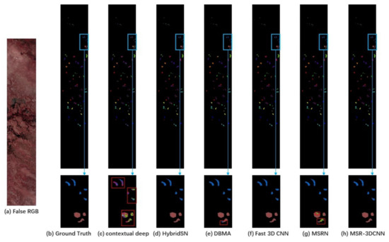
Figure 10. Results of the BO dataset using 10% samples for training and $\left(9\times 9\right)$ patch size.

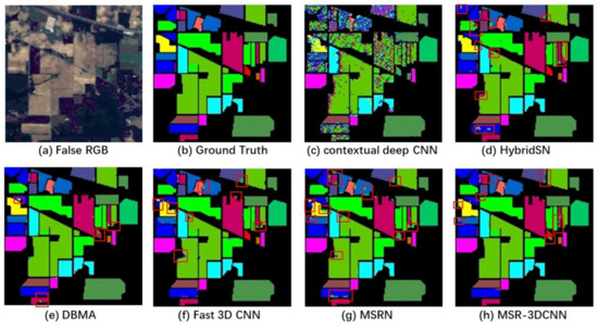
Figure 11. Results of the IP dataset using 10% samples for trainingand $\left(9\times 9\right)$ patch size.

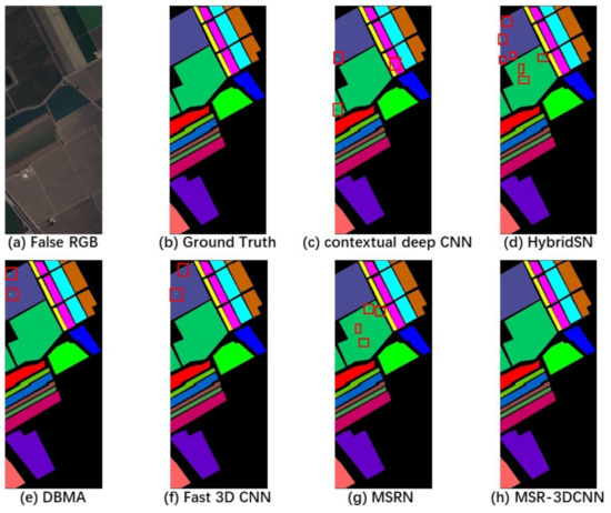
Figure 12. Results of the SA dataset using 10% samples for training and $\left(9\times 9\right)$ patch size.

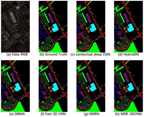
Figure 13. Results of the PU dataset using 10% samples for training and $\left(9\times 9\right)$ patch size.

Figure 14, Figure 15, Figure 16 and Figure 17 show the confusion matrices [38,39] between ground truth on the experimental datasets and the predicted results of MSR-3DCNN using 10% training samples and $\left(9\times 9\right)$ patch size. These confusion matrices show the classification status of each category on each dataset of MSR-3DCNN, which is consistent with the visual evaluation of the classification results. MSR-3DCNN can obtain accurate classifications for basically all the classes, including these with very limited amount of samples.

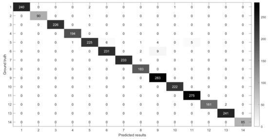
Figure 14. The confusion matrix between the predicted results of MSR-3DCNN and ground truth on the BO dataset using 10% samples for training and $\left(9\times 9\right)$ patch size.

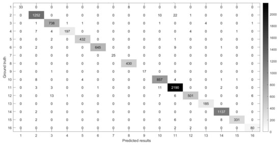
Figure 15. The confusion matrix between the predicted results of MSR-3DCNN and ground truth on the IP dataset using 10% samples for training and $\left(9\times 9\right)$ patch size.

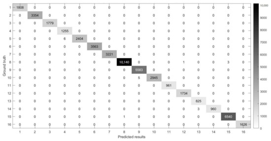
Figure 16. The confusion matrix between the predicted results of MSR-3DCNN and ground truth on the SA dataset using 10% samples for training and $\left(9\times 9\right)$ patch size.

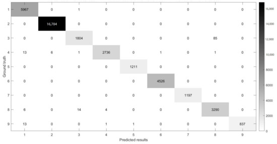
Figure 17. The confusion matrix between the predicted results of MSR-3DCNN and ground truth on the PU dataset using 10% samples for training and $\left(9\times 9\right)$ patch size.

5. Conclusions

In this paper, we propose a Multiple Spectral Resolution 3D Convolutional Neural Network for HSI classification. As compared to the other researches about HSI classification models, more attention has been paid to the spectral dimension of HSIs in our model. The idea of dilated convolution and multi-scale fusion has been expanded from the spatial dimension to the spectral dimension; therefore, two novel designs—spectral dilated convolution and multiple spectral resolution fusion—have been proposed. Using these two novel designs, the proposed MSR-3DCNN can theoretically have better spectral information extraction and analysis capabilities, and therefore may be less demanding on the spatial information of HSIs.The theoretical advantage of MSR-3DCNN has been verified in our comparative experiments. As shown by the experimental results, MSR-3DCCNN is much more insensitive to the change of patch size and has better performance under small patch size. Note that MSR-3DCNN showed advantages in various experimental datasets, showing a strong applicability, which is of great significance for the application of a new generation of hyperspectral sensors. In the future, we plan to further improve this approach by reducing the calculations as well as applying it to the new generation of hyperspectral systems.

References

- Signoroni, A.; Savardi, M.; Baronio, A.; Benini, S. Deep learning meets hyperspectral image analysis: A multidisciplinary review. J. Imaging 2019, 5, 52. [Google Scholar] [CrossRef]
- Teke, M.; Deveci, H.S.; Haliloğlu, O.; Gürbüz, S.Z.; Sakarya, U. A short survey of hyperspectral remote sensing applications in agriculture. In Proceedings of the 2013 6th International Conference on Recent Advances in Space Technologies (RAST), Istanbul, Turkey, 12–14 June 2013; pp. 171–176. [Google Scholar] [CrossRef]
- Adão, T.; Hruška, J.; Pádua, L.; Bessa, J.; Peres, E.; Morais, R.; Sousa, J.J. Hyperspectral Imaging: A Review on UAV-Based Sensors, Data Processing and Applications for Agriculture and Forestry. Remote Sens. 2017, 9, 1110. [Google Scholar] [CrossRef]
- Paoletti, M.; Haut, J.; Plaza, J.; Plaza, A. Deep learning classifiers for hyperspectral imaging: A review. ISPRS J. Photogramm. Remote Sens. 2019, 158, 279–317. [Google Scholar] [CrossRef]
- Long, J.; Shelhamer, E.; Darrell, T. Fully convolutional networks for semantic segmentation. In Proceedings of the IEEE Conference on Computer Vision and Pattern Recognition, Boston, MA, USA, 7–12 June 2015; pp. 3431–3440. [Google Scholar]
- Krizhevsky, A.; Sutskever, I.; Hinton, G.E. Imagenet classification with deep convolutional neural networks. Commun. ACM 2017, 60, 84–90. [Google Scholar] [CrossRef]
- He, K.; Zhang, X.; Ren, S.; Sun, J. Deep residual learning for image recognition. In Proceedings of the IEEE Conference on Computer Vision and Pattern Recognition, Las Vegas, NV, USA, 27–30 June 2016; pp. 770–778. [Google Scholar]
- Chen, Y.; Jiang, H.; Li, C.; Jia, X.; Ghamisi, P. Deep feature extraction and classification of hyperspectral images based on convolutional neural networks. IEEE Trans. Geosci. Remote Sens. 2016, 54, 6232–6251. [Google Scholar] [CrossRef]
- Zhao, W.; Du, S. Spectral–Spatial Feature Extraction for Hyperspectral Image Classification: A Dimension Reduction and Deep Learning Approach. IEEE Trans. Geosci. Remote Sens. 2016, 54, 4544–4554. [Google Scholar] [CrossRef]
- Lee, H.; Kwon, H. Going deeper with contextual CNN for hyperspectral image classification. IEEE Trans. Image Process. 2017, 26, 4843–4855. [Google Scholar] [CrossRef]
- Roy, S.K.; Krishna, G.; Dubey, S.R.; Chaudhuri, B.B. HybridSN: Exploring 3-D–2-D CNN feature hierarchy for hyperspectral image classification. IEEE Geosci. Remote Sens. Lett. 2019, 17, 277–281. [Google Scholar] [CrossRef]
- Ma, W.; Yang, Q.; Wu, Y.; Zhao, W.; Zhang, X. Double-branch multi-attention mechanism network for hyperspectral image classification. Remote Sens. 2019, 11, 1307. [Google Scholar] [CrossRef]
- Ahmad, M. A fast 3D CNN for hyperspectral image classification. arXiv 2020, arXiv:2004.14152. [Google Scholar]
- Zhang, X.; Wang, T.; Yang, Y. Hyperspectral Images Classification Based on Multi-scale Residual Network. arXiv 2020, arXiv:2004.12381. [Google Scholar]
- Datt, B.; McVicar, T.R.; Van Niel, T.G.; Jupp, D.L.; Pearlman, J.S. Preprocessing EO-1 Hyperion hyperspectral data to support the application of agricultural indexes. IEEE Trans. Geosci. Remote Sens. 2003, 41, 1246–1259. [Google Scholar] [CrossRef]
- Pignatti, S.; Palombo, A.; Pascucci, S.; Romano, F.; Santini, F.; Simoniello, T.; Umberto, A.; Vincenzo, C.; Acito, N.; Diani, M.; et al. The PRISMA hyperspectral mission: Science activities and opportunities for agriculture and land monitoring. In Proceedings of the 2013 IEEE International Geoscience and Remote Sensing Symposium (IGARSS), Melbourne, Australia, 21–26 July 2013; pp. 4558–4561. [Google Scholar]
- Guanter, L.; Kaufmann, H.; Segl, K.; Foerster, S.; Rogass, C.; Chabrillat, S.; Kuester, T.; Hollstein, A.; Rossner, G.; Chlebek, C.; et al. The EnMAP spaceborne imaging spectroscopy mission for earth observation. Remote Sens. 2015, 7, 8830–8857. [Google Scholar] [CrossRef]
- Ji, S.; Xu, W.; Yang, M.; Yu, K. 3D convolutional neural networks for human action recognition. IEEE Trans. Pattern Anal. Mach. Intell. 2012, 35, 221–231. [Google Scholar] [CrossRef]
- Zhao, H.; Shi, J.; Qi, X.; Wang, X.; Jia, J. Pyramid scene parsing network. In Proceedings of the IEEE Conference on Computer Vision and Pattern Recognition, Honolulu, HI, USA, 21–26 July 2017; pp. 2881–2890. [Google Scholar]
- Szegedy, C.; Liu, W.; Jia, Y.; Sermanet, P.; Reed, S.; Anguelov, D.; Erhan, D.; Vanhoucke, V.; Rabinovich, A. Going deeper with convolutions. In Proceedings of the IEEE Conference on Computer Vision and Pattern Recognition, Boston, MA, USA, 7–12 June 2015; pp. 1–9. [Google Scholar]
- Yu, F.; Koltun, V.; Funkhouser, T. Dilated residual networks. In Proceedings of the IEEE Conference on Computer Vision and Pattern Recognition, Honolulu, HI, USA, 21–26 July 2017; pp. 472–480. [Google Scholar]
- LeCun, Y.; Bottou, L.; Bengio, Y.; Haffner, P. Gradient-based learning applied to document recognition. Proc. IEEE 1998, 86, 2278–2324. [Google Scholar] [CrossRef]
- Bengio, Y.; LeCun, Y. Scaling learning algorithms towards AI. Large-Scale Kernel Mach. 2007, 34, 1–41. [Google Scholar]
- Peng, C.; Zhang, X.; Yu, G.; Luo, G.; Sun, J. Large kernel matters–improve semantic segmentation by global convolutional network. In Proceedings of the IEEE Conference on Computer Vision and Pattern Recognition, Honolulu, HI, USA, 21–26 July 2017; pp. 4353–4361. [Google Scholar]
- Srivastava, N.; Hinton, G.; Krizhevsky, A.; Sutskever, I.; Salakhutdinov, R. Dropout: A simple way to prevent neural networks from overfitting. J. Mach. Learn. Res. 2014, 15, 1929–1958. [Google Scholar]
- Santurkar, S.; Tsipras, D.; Ilyas, A.; Madry, A. How does batch normalization help optimization? arXiv 2018, arXiv:1805.11604. [Google Scholar]
- Wold, S.; Esbensen, K.; Geladi, P. Principal component analysis. Chemom. Intell. Lab. Syst. 1987, 2, 37–52. [Google Scholar] [CrossRef]
- Abdi, H.; Williams, L.J. Principal component analysis. Wiley Interdiscip. Rev. Comput. Stat. 2010, 2, 433–459. [Google Scholar] [CrossRef]
- Ozdemir, A.; Polat, K. Deep learning applications for hyperspectral imaging: A systematic review. J. Inst. Electron. Comput. 2020, 2, 39–56. [Google Scholar] [CrossRef]
- Vali, A.; Comai, S.; Matteucci, M. Deep learning for land use and land cover classification based on hyperspectral and multispectral earth observation data: A review. Remote Sens. 2020, 12, 2495. [Google Scholar] [CrossRef]
- Audebert, N.; Le Saux, B.; Lefèvre, S. Deep learning for classification of hyperspectral data: A comparative review. IEEE Geosci. Remote Sens. Mag. 2019, 7, 159–173. [Google Scholar] [CrossRef]
- Abadi, M.; Barham, P.; Chen, J.; Chen, Z.; Davis, A.; Dean, J.; Devin, M.; Ghemawat, S.; Irving, G.; Isard, M.; et al. Tensorflow: A system for large-scale machine learning. In Proceedings of the 12th {USENIX} Symposium on Operating Systems Design and Implementation ({OSDI} 16), Savannah, GA, USA, 2–4 November 2016; pp. 265–283. [Google Scholar]
- Alberg, A.J.; Park, J.W.; Hager, B.W.; Brock, M.V.; Diener-West, M. The use of “overall accuracy” to evaluate the validity of screening or diagnostic tests. J. Gen. Intern. Med. 2004, 19, 460–465. [Google Scholar] [CrossRef] [PubMed]
- Fung, T.; LeDrew, E. For change detection using various accuracy. Photogramm. Eng. Remote Sens. 1988, 54, 1449–1454. [Google Scholar]
- Goutte, C.; Gaussier, E. A probabilistic interpretation of precision, recall and F-score, with implication for evaluation. In Proceedings of the European Conference on Information Retrieval, Santiago de Compostela, Spain, 21–23 March 2005; Springer: Berlin/Heidelberg, Germany, 2005; pp. 345–359. [Google Scholar]
- Wang, Y.; Yu, W.; Fang, Z. Multiple Kernel-Based SVM Classification of Hyperspectral Images by Combining Spectral, Spatial, and Semantic Information. Remote Sens. 2020, 12, 120. [Google Scholar] [CrossRef]
- Polikar, R. Ensemble learning. In Ensemble Machine Learning; Springer: Berlin/Heidelberg, Germany, 2012; pp. 1–34. [Google Scholar]
- Deng, X.; Liu, Q.; Deng, Y.; Mahadevan, S. An improved method to construct basic probability assignment based on the confusion matrix for classification problem. Inf. Sci. 2016, 340, 250–261. [Google Scholar] [CrossRef]
- Foody, G.M. Status of land cover classification accuracy assessment. Remote Sens. Environ. 2002, 80, 185–201. [Google Scholar] [CrossRef]
Publisher’s Note: MDPI stays neutral with regard to jurisdictional claims in published maps and institutional affiliations. |
© 2021 by the authors. Licensee MDPI, Basel, Switzerland. This article is an open access article distributed under the terms and conditions of the Creative Commons Attribution (CC BY) license (http://creativecommons.org/licenses/by/4.0/).