Communication

Atmospheric Correction of Airborne Hyperspectral CASI Data Using Polymer, 6S and FLAASH

1
Department of Civil and Environmental Engineering, Pusan National University, Pusan 43241, Korea
2
Chongqing Institute of Surveying and Monitoring for Planning and Natural Resources, Chongqing 400120, China
3
School of Economics and Management, Tiangong University, Tianjin 300387, China
4
Institute of Environmental Studies, University of Karachi, Karachi 75270, Pakistan
5
Lamont-Doherty Earth Observatory, Marine Biology and Paleo Environment, Columbia University, Palisades, NY 10964-8000, USA
*
Author to whom correspondence should be addressed.
Remote Sens. 2021, 13(24), 5062; https://doi.org/10.3390/rs13245062
Submission received: 8 November 2021 / Revised: 11 December 2021 / Accepted: 11 December 2021 / Published: 13 December 2021
(This article belongs to the Special Issue Advances in Remote Sensing of the Inland and Coastal Water Zones)

Abstract

:
Airborne hyperspectral data play an important role in remote sensing of coastal waters. However, before their application, atmospheric correction is required to remove or reduce the atmospheric effects caused by molecular and aerosol scattering and absorption. In this study, we first processed airborne hyperspectral CASI-1500 data acquired on 4 May 2019 over the Uljin coast of Korea with Polymer and then compared the performance with the other two widely used atmospheric correction approaches, i.e., 6S and FLAASH, to determine the most appropriate correction technique for CASI-1500 data in coastal waters. Our results show the superiority of Polymer over 6S and FLAASH in deriving the Rrs spectral shape and magnitude. The performance of Polymer was further evaluated by comparing CASI-1500 Rrs data with those obtained from the MODIS-Aqua sensor on 3 May 2019 and processed using Polymer. The spectral shapes of the derived Rrs from CASI-1500 and MODIS-Aqua matched well, but the magnitude of CASI-1500 Rrs was approximately 0.8 times lower than MODIS Rrs. The possible reasons for this difference were time difference (1 day) between CASI-1500 and MODIS data, higher land adjacency effect for MODIS-Aqua than for CASI-1500, and possible errors in MODIS Rrs from Polymer.

Graphical Abstract

1. Introduction

Remote sensing is an effective tool for monitoring coastal waters, which are complex and highly variable ecosystems. Airborne hyperspectral sensors have several advantages over spaceborne sensors, and thus they play a vital role in remote sensing. First, imagery from airborne sensors are of a higher spatial resolution. For instance, the Compact Airborne Spectrographic Imager (CASI)-1500 has a spatial resolution that varies with flight altitude and can be 1 m × 1 m if the aircraft is at an altitude of approximately 2 km above the ground, whereas the spaceborne sensors such as SeaWiFS (Sea-viewing Wide Field-of-view Sensor) and MODIS (MODerate resolution Imaging Spectroradiometer) have a spatial resolution of 1 km × 1 km. This higher spatial resolution of airborne hyperspectral sensors makes them more desirable for coastal water applications [1,2].
The second advantage is that most airborne hyperspectral sensors are programmable in terms of the number and locations of spectral channels and their bandwidths. For example, 36 spectral bands may be acquired with 1 m × 1 m spatial resolution and a flight speed of 120 knots, whereas 48 spectral bands are possible at a flight speed of 90 knots. Therefore, for a given location, it is possible to adjust spectral channels and spectral resolutions as desired [3]. Another advantage is that the timing of airborne data acquisition can be controlled, so adverse weather conditions such as cloud cover, rain, and haze can be avoided, whereas data collected from spaceborne sensors under these conditions are often invalid. Disadvantages of airborne remote sensing compared to satellite and in situ sampling include high cost and lengthy data processing time due to large data volume. Additionally, airborne remote sensing has smaller spatial coverage than satellite sampling. Despite this, airborne remote sensing is particularly useful for mapping coastal waters, as spatial and spectra resolutions are demanding in these areas.
However, atmospheric correction is critical before the quantitative application of airborne hyperspectral data. Atmospheric correction removes or reduces the effects caused by molecular and particular scattering and absorption, thus converting the radiances measured by the sensors to remote sensing reflectances (Rrs) of the target surfaces [4,5]. In the past three decades, atmospheric correction algorithms have been developed that range from empirical models to rigorous physically based radiative transfer models [6,7,8,9,10,11,12,13]. Some of the most popular atmospheric correction approaches include Polymer (POLYnomial based algorithm applied to MERIS), 6S (Second Simulation of a Satellite Signal in the Solar Spectrum), FLAASH (Fast Line-of-sight Atmospheric Analysis of Spectral Hypercubes), and ATCOR (ATmospheric CORrection) [14,15,16,17]. A few studies were carried that compare several radiative transfer models using medium and high-resolution data. For instance, Eugenio et al. [18] implemented 6S, FLAASH, and ATCOR; and Marcello et al. [19] implemented DOS (Dark Object Subtraction), QUAC (Quick Atmospheric Correction), 6S, FLAASH, and ATCOR for high-resolution WordView-2, a satellite-based imaging system with a spatial resolution of 0.46 m in the panchromatic (PAN) band and 1.84 m in eight multispectral (MS) channels. Nguyen et al. [20] evaluated 6S, FLAASH, and DOS using Landsat ETM+, which has a spatial resolution of 30 m for band 1 to 7 and a resolution of 15 m for the panchromatic band 8. In general, radiative transfer models outperform empirical methods, but no single algorithm performs best in all scenarios [18].
In this study, the performance of three atmospheric correction algorithms, i.e., Polymer, 6S, and FLAASH, were evaluated using a CASI-1500 imagery acquired on 4 May 2019 over the Uljin coast, the southeastern coast of Korea (Figure 1). Polymer was purposed to recovering ocean colour from the top-of-atmosphere signal measured by satellite sensors in the visible spectrum. One of the strengths of this algorithm is the possibility to recover ocean colour in the presence of sun glint. It has been applied to multiple sensors from ESA (MERIS/ENVISAT, MSI/Sentinel-2, and OLCI/Sentinel-3), NASA (SeaWiFS, MODIS/Aqua, VIIRS), and the Korean Geostationary Ocean Colour Imager (GOCI) [14,21,22,23]. However, to our knowledge, Polymer has not yet been applied to airborne hyperspectral sensors. It is to be expected that the atmospheric correction procedures useful for satellites can be valid for airborne sensors, although satellites and airborne sensors are at different altitudes. The 6S algorithm is one of the most widely used, rigorously validated, and heavily documented radiative transfer codes [24], although it is mainly applied to satellite sensors as well [18,25,26,27]. FLAASH has been applied to airborne hyperspectral data [28]. However, it does not separate the surface Fresnel reflectance from the target reflectance, which is acceptable for land areas but invalid for water areas [29]. In addition, FLAASH uses homogeneous aerosol properties derived from a dark target for the entire scene [30].
The waters along the Uljin coast are shallow with water depths < 20 m (Figure 1b). Seaweed is the dominant primary producer in this ecosystem, but whitening of coralline algae has adversely affected this region. Therefore, whitening detection is necessary to better understand the degradation of the ecosystem and help the local government to develop mitigation measures. In a recent study, Kim et al. [31] investigated the whitening of the Uljin coast via benthic mapping using CASI-1500 data, atmospherically corrected using FLAASH. However, the resulting CASI-1500 Rrs data were not validated as no field measurements of Rrs were available.
The objective of this study was to find the most suitable atmospheric correction algorithm to apply to CASI-1500 data for future studies in shallow coastal ecosystems. Additionally, for the first time, we applied Polymer to airborne hyperspectral data.

2. Materials and Methods

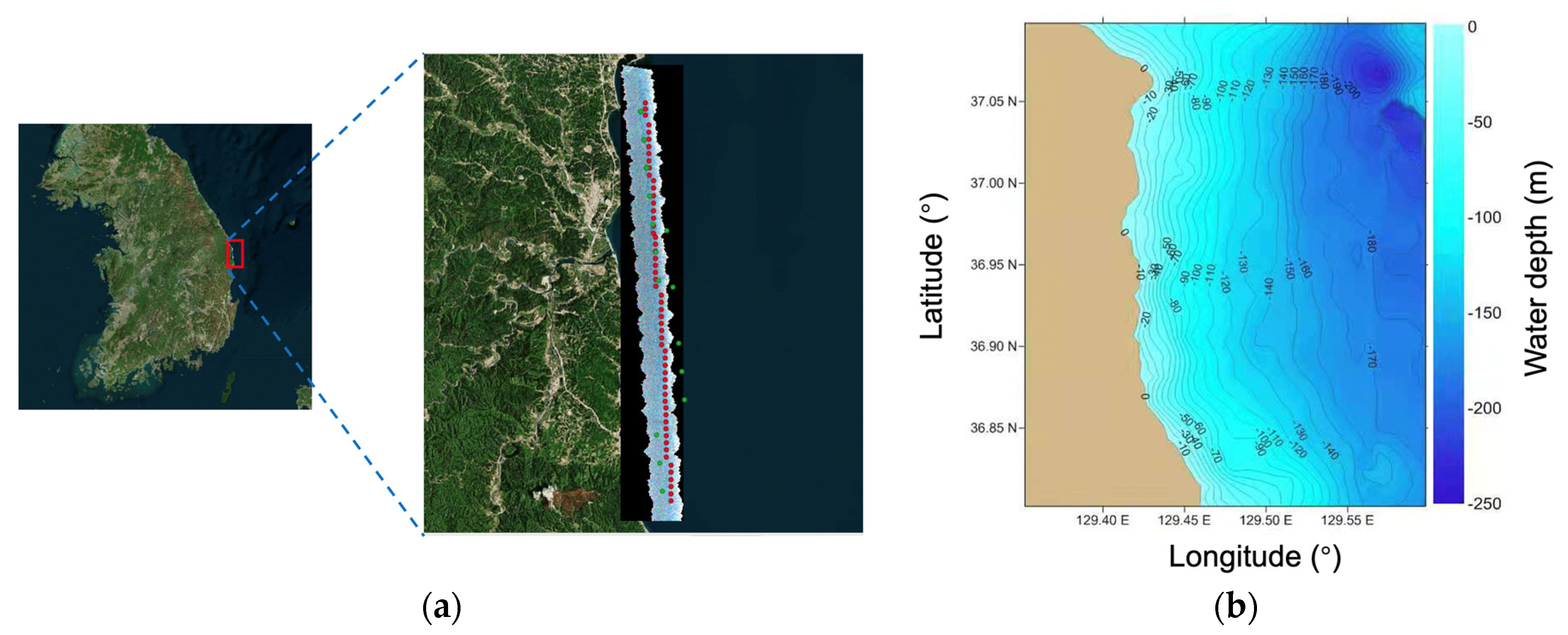
2.1. Airborne Hyperspectral Data

CASI-1500 hyperspectral data were acquired at 14:17:47 (+9 h GMT) on 4 May 2019, for an area ranging from 36.84°N to 37.05°N latitude and 129.41°E to 129.46°E longitude (Figure 1). The data were collected at an altitude of 2 km with a spatial resolution of 1 m across 48 spectral bands with a full width at half maximum of 7.2 nm (Table 1).
Pre-processing of the CASI-1500 data included radiometric calibration, which converted digital number (DN) into spectral radiance unit (SRU, μw cm−2 sr−1 nm−1) with a scale factor of 1000, and geometric calibration using the GEOCORR program, which geo-referenced the data to UTM WGS84 [31]. Use of CASI-1500 also required use of inputs from MODIS-Aqua described in Section 2.2.

2.2. Satellite and Reanalysis Data

MODIS (Moderate Resolution Imaging Spectroradiometer), a key instrument aboard the Aqua (EOS PM) satellite (MODIS/Aqua), has a spatial and temporal resolution of 1 km and 1 day, respectively. The Level-1A data at 5:00 (GMT) on 3 May 2019 were obtained from the NASA Goddard Space Flight Center. They were converted into Level-1B data using the OCSSW tools in the SeaDAS 7.5.3 software, and finally into Level-1C data that included all the necessary radiometric corrections using the l2gen command in the Polymer codes [14,21]. The Level-1C data were further processed to Level-2 data using the Polymer approach. These Level-2 Rrs data had a spatial resolution of 1 km at bands 412, 443, 488, 531, 547, 667, 678, 748, 859, and 869 nm, 500 m at bands 469 and 555 nm, and 250 m at band 645 nm. MODIS Rrs data at all bands except for band 678 were compared with the CASI Rrs data obtained after applying the Polymer atmospheric correction to radiance data. The Rrs at band 678 was not compared because Polymer failed to retrieve CASI Rrs at this band.
It should be noted that the MODIS and CASI data were acquired on different dates (1 day difference) because no valid MODIS data were available for the 4 May 2019 when the CASI data were collected. Therefore, when comparing the MODIS and CASI Rrs data, we were mindful that this time difference needed to be considered in our analysis. In addition, the spatial resolutions of CASI and MODIS sensors are much different (1 m vs. 1 km). To compare CASI and MODIS Rrs, we averaged CASI values within the MODIS 1 km pixel.
Next, the 6S atmospheric correction approach was applied to MODIS atmosphere and chlorophyll-a (Chl-a) products as well as reanalysis Modern-Era Retrospective analysis for Research and Applications, Version 2 (MERRA-2) products provided by the National Aeronautics and Space Administration Goddard Space Flight Center. Specifically, we used two MODIS atmosphere products, including MYD05 (water vapour) and MYD07 (total ozone) at 4:05 (GMT) on 4 May 2019, approximately 1 h before the acquisition of CASI-1500 data. The spatial resolution of MYD05 and MYD07 was 0.05°. As the MODIS aerosol product from MYD04 (aerosol optical thickness at 550 nm, aot_550) was not available for the same day, we used the hourly MERRA-2 aerosol product (Total Aerosol Extinction AOT [550 nm]) with a much coarser spatial resolution of 0.5° × 0.625°. Additionally, we also used MODIS Level-2 Chl-a product on 3 May 2019 (5:00 GMT) and hourly MERRA-2 wind speed product (U2M and V2M) on 4 May 2019. The spatial resolution of these products was 1 km × 1 km and 0.5° × 0.625°, respectively.

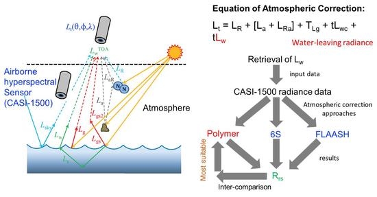
2.3. Polymer Atmospheric Correction Approach

Polymer proved advantageous in recovering pixels under sun glint compared to traditional atmospheric correction algorithms. In addition, it uses a polynomial function of wavelength (λ) and an ocean reflectance model to calculate water surface reflectance based on a spectral matching technique. A brief summary of the Polymer procedure is as follows:
First, an initial atmospheric correction is carried out for the top-of-atmosphere reflectance ( ρ T O A ( λ ) ) which is decomposed according to the following equation:
  ρ T O A ( λ ) = t o z ( λ ) [ ρ m o l ( λ ) + T ( λ ) ρ g l i + ρ a e r ( λ ) + ρ c o u p l ( λ ) + t ( λ ) ρ w + ( λ ) ]
where t o z ( λ ) is the transmittance of ozone; ρ m o l ( λ ) , ρ g l i , ρ a e r ( λ ) , ρ c o u p l ( λ ) , and ρ w + ( λ ) are the reflectance of Rayleigh scattering, sun glint, non-absorbing aerosols, and the various couplings between sun glint, molecules, and aerosols, as well as of the water above the water-air interface, respectively; T ( λ ) and t ( λ ) are the direct transmission factors and the total (direct and diffuse) transmission for atmospheric scattering, respectively. The t o z ( λ ) ,   ρ m o l ( λ ) , and ρ g l i were obtained using the Successive Order of Scattering (SOS) radiative transfer model in [14].
After the initial atmospheric correction, the remaining term ( ρ ( λ ) ) is expressed by the following equation:
ρ ( λ ) = ρ g l i ( λ ) + ρ a e r ( λ ) + ρ c o u p l ( λ ) + t ( λ ) ρ w + ( λ )
Furthermore, the first three terms and the last term are modelled by T 0 ( λ ) c 0 + c 1 λ 1 + c 2 λ 4 and ρ w m o d + ( [ c h l ] , b b N C , λ ) , respectively. The T 0 ( λ ) is a transmission factor that can be calculated using the formula in [14]. The variables Chl and bbNC represent the chlorophyll-a concentration and the backscattering coefficient of non-covarying particles, respectively. Therefore, ρ ( λ ) is also expressed by the following equation:
ρ ( λ ) = T 0 ( λ ) c 0 + c 1 λ 1 + c 2 λ 4 + t ( λ ) ρ w m o d + ( [ c h l ] , b b N C , λ )
The spectral matching technique retrieves c0, c1, c2, chl, and bbNC, and finally ρ w + ( λ ) is obtained based on these parameters.
To quality control the MODIS-Aqua Rrs after application of the Polymer atmospheric algorithm, several criteria were established to exclude the Rrs data that did not meet our strict requirements: (1) High sun glint (Lgn > 0.005 sr−1), where Lgn is a sun glint coefficient calculated with the model by Cox and Munk [32] and wind [33]; (2) Thick clouds (ρTOA(869) − toz(869)ρmol(869) > 0.027); (3) high air mass (1/cos(θs) + 1/cos(θv) > 5), where θs and θv are solar zenith angle and sensor zenith angle, respectively; and (4) θs > 88°. The criteria for quality control of CASI Rrs after application of the Polymer atmospheric algorithm were the same as for MODIS-Aqua Rrs but the band used for (2) was 873 nm, which is the closest band to the MODIS-Aqua 869 nm band.
The main modification that we undertook when using Polymer for processing CASI data is that we used the 6S output parameters, including t o z ( λ ) , ρ m o l ( λ ) , ρ g l i , transmission of Rayleigh scattering ( T m o l ( λ ) ), and Rayleigh optical thickness from the top-of-atmosphere to sensor (τm_sensor(λ)), and total Rayleigh optical thickness (τm_total(λ)) from the top-of-atmosphere to sea surface, for the initial atmospheric correction and Polymer atmospheric correction model. The difference between τm_total(λ) and τm_sensor(λ) (τm_total(λ) − τm_sensor(λ)) is the Rayleigh optical thickness from sensor to sea surface.
The CASI radiance data were converted into apparent reflectance using the following equation:
ρ * ( λ ) = L / E s _ s e n s o r
where L and Es_sensor represent the CASI radiance and the simulated solar downwelling irradiance at the sensor altitude, respectively.
We calculated Es_sensor using the following equations [14,34]:
E s _ s e n s o r ( λ ) = E s o l d i r ( λ ) + E s o l d i f f ( λ )
E s o l d i r ( λ ) = μ s E s _ T O A T 0 d i r ( λ )  
E s o l d i f f ( λ ) = μ s E s _ T O A T 0 d i f f ( λ )  
E s _ T O A = λ 1 λ 2 E ( λ ) S ( λ ) d λ λ 1 λ 2 S ( λ ) d λ
    T 0 d i r ( λ ) = e x p [ ( τ m _ t o t a l ( λ ) ) τ m _ s e n s o r ( λ ) ) × ( 1 μ s + 1 μ v ) ]
T 0 d i f f ( λ ) = e x p [ 0.5 × ( τ m _ t o t a l ( λ ) τ m _ s e n s o r ( λ ) ) × ( 1 μ s + 1 μ v ) ]
where E s o l d i r ( λ ) and E s o l d i f f ( λ ) are the direct and diffuse solar downwelling irradiance at the sensor altitude, respectively; Es_TOA is the solar downwelling irradiance at the top-of-atmosphere; T 0 d i r ( λ ) and T 0 d i f f ( λ ) are the direct and diffuse transmittance factors, respectively; E(λ) and S(λ) are the 1985 Wehrli Standard Extraterrestrial Solar Irradiance Spectrum and spectral response function of CASI, respectively; λ1 and λ2 are the start and end wavelength of each CASI band, respectively; and μs and μv are the cosine of solar zenith angle and sensor zenith angle, respectively.

2.4. 6S Atmospheric Correction Approach

The 6S algorithm is one of the most widely used, rigorously validated, and elaborately documented radiative transfer codes [24]. The vector version of 6S was used in this study and it accounts for radiation polarization, in contrast to the scalar version of 6S. Accuracy of the atmospheric correction results by 6S is affected by the input atmospheric parameters, including the aerosol optical thickness and total amount of water vapour and ozone. However, field measurements of these parameters are often unavailable. Therefore, we used satellite and reanalysis atmospheric products (as described in Section 2.2) in this study. Furthermore, 6S simulated the atmospheric parameters at the airborne sensor altitude that were used as the final 6S input.
The parameter settings of 6S for the CASI-1500 imagery are described as below (Table 2).
The solar zenith angle and solar azimuth angle were calculated from one-pixel location in the CASI-1500 imagery using Pysolar codes. Sensor zenith angle and sensor azimuth angle were calculated for each pixel. The former was obtained by dividing the DN values of the CASI-1500 NAD (NADIR Channel) imagery by 1000, whereas the latter using the formula acquired from https://www.omnicalculator.com/other/azimuth#what-is-the-azimuth, accessed on 25 August 2021. In general, the sensor azimuth angles were 0° for the nadir view pixels, 90° for the pixels on the left side of the nadir view pixels, and 270° for the pixels on the right side of the nadir view pixels. As the location points for validation (red symbols in Figure 1) were generally on the right side of the nadir view pixels, the sensor azimuth angle was set to be 270°. For total water vapour, total ozone, and Chl-a concentration, averaged values from the pixels covering the CASI-1500 imagery were used. For aot_550 and wind speed, a single value from the pixel covering the whole CASI-1500 imagery was used. In addition, the aerosol model was chosen to be Maritime based on the location and climate of the study area. Finally, sea water salinity was set to be 34.3 ppt for each pixel.
The 6S model is expressed by the following equation [18,35]. Reference to wavelength (λ) is omitted for clarity of the equation:
      ρ T O A ( θ s , θ v , Δ ϕ ) = t g ( θ s , θ v ) { ρ a ( θ s , θ v , Δ ϕ ) + [ e τ μ s + t d ( θ s ) ] ρ s u e τ μ v + ρ e t d ( θ v ) 1 ρ e S }
where ρ T O A , ρ a , ρ s u ,   a n d   ρ e   represent the top-of-atmosphere reflectance, atmospheric reflectance, surface reflectance, and a homogenous environment of reflectance, respectively; Δ ϕ represents the difference between solar and sensor azimuth; t g   represents   the   total transmissivity of the gases, considering the absorption of different gases; τ   represents the atmospheric thickness; t d ( θ s )   and   t d ( θ v ) represent the diffuse transmittance of the atmosphere; S represents the spherical albedo of the atmosphere; and the 1 ρ e S term considers the multiple scatterings between the surface and the atmosphere.

2.5. FLAASH Atmospheric Correction Approach

FLAASH is available in ENVI and it incorporates MODTRAN4 radiative transfer code [34]. The FLAASH model is expressed by the following equation. Again, reference wavelength (λ) is also omitted for simplicity:
  L = ( A ρ 1 ρ e S ) + ( B ρ e 1 ρ e S ) + L a
where L represents the radiance at the sensor pixel; ρ represents the pixel surface reflectance; ρ e represents an average surface reflectance for the pixel and the surrounding region; S represents the spherical albedo of the atmosphere; L a represents the radiance backscattered by the atmosphere; and A and B are coefficients that depend on atmospheric and geometric conditions.
For the FLAASH parameter setting, any of the standard MODTRAN model atmosphere and aerosol types can be chosen to represent a scene and a unique MODTRAN solution is computed for each image. In this study, mid-latitude summer and maritime were selected for the atmospheric and aerosol models, respectively. The initial visibility value was obtained from the 6S simulation, which used the reanalysis aot_550 as the input data. Water vapour was retrieved using the water absorption feature at 940 nm.
The parameter settings of FLAASH applied to CASI-1500 imagery are described in Table 3.

2.6. Statistical Analysis

To quantitatively measure the spectral similarity between the CASI-1500 and MODIS Rrs spectra obtained by Polymer, we calculated the cosine distance using the following equation [23,36]:
cos ( α ) = i N ( R r s C A S I , i R r s M O D I S , i ) i N ( R r s C A S I , i ) 2 i N ( R r s M O D I S , i ) 2
where α represents the angle between the CASI Rrs spectrum (RrsCASI,i ) and MODIS Rrs spectrum (RrsMODIS,i). A closer match of the two spectra is indicated by a smaller α and a bigger cos(α).

3. Results

The results from applying the atmospheric correction approaches—Polymer, 6S, and FLAASH—to CASI-1500 data were compared. MODIS data were processed with Polymer as the atmospheric algorithm was used to evaluate the performance of Polymer for CASI-1500 data.

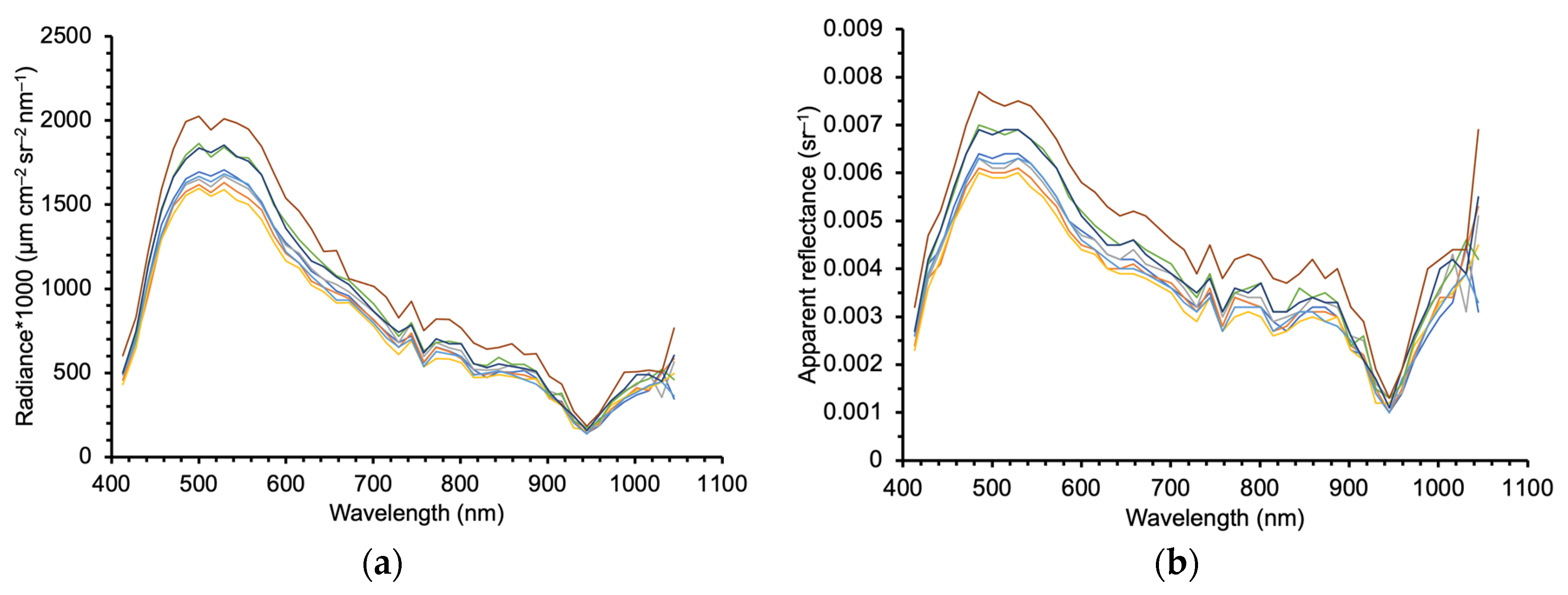
3.1. CASI-1500 Radiance and Apparent Reflectance

CASI-1500 radiance data (Figure 1a) were first converted into apparent reflectance data and then processed using Polymer to obtain the CASI-1500 Rrs data.
Radiance data were collected from eight locations, i.e., No. 1, No. 9, No. 17, No. 25, No. 33, No. 41, No. 49, and No. 57 shown as evenly distributed (from top to bottom) red symbols on the CASI radiance image in Figure 1. The radiance spectra (Figure 2a), had similar spectral shapes but different magnitudes. Specifically, the spectra peaked at the green band near 500 nm, which is typical for coastal waters. Several spectral valleys seen near 720 nm, 760 nm, 820 nm, and 940 nm are due to absorption by water vapour and oxygen. The apparent radiance data had similar spectral shapes as the radiance data.

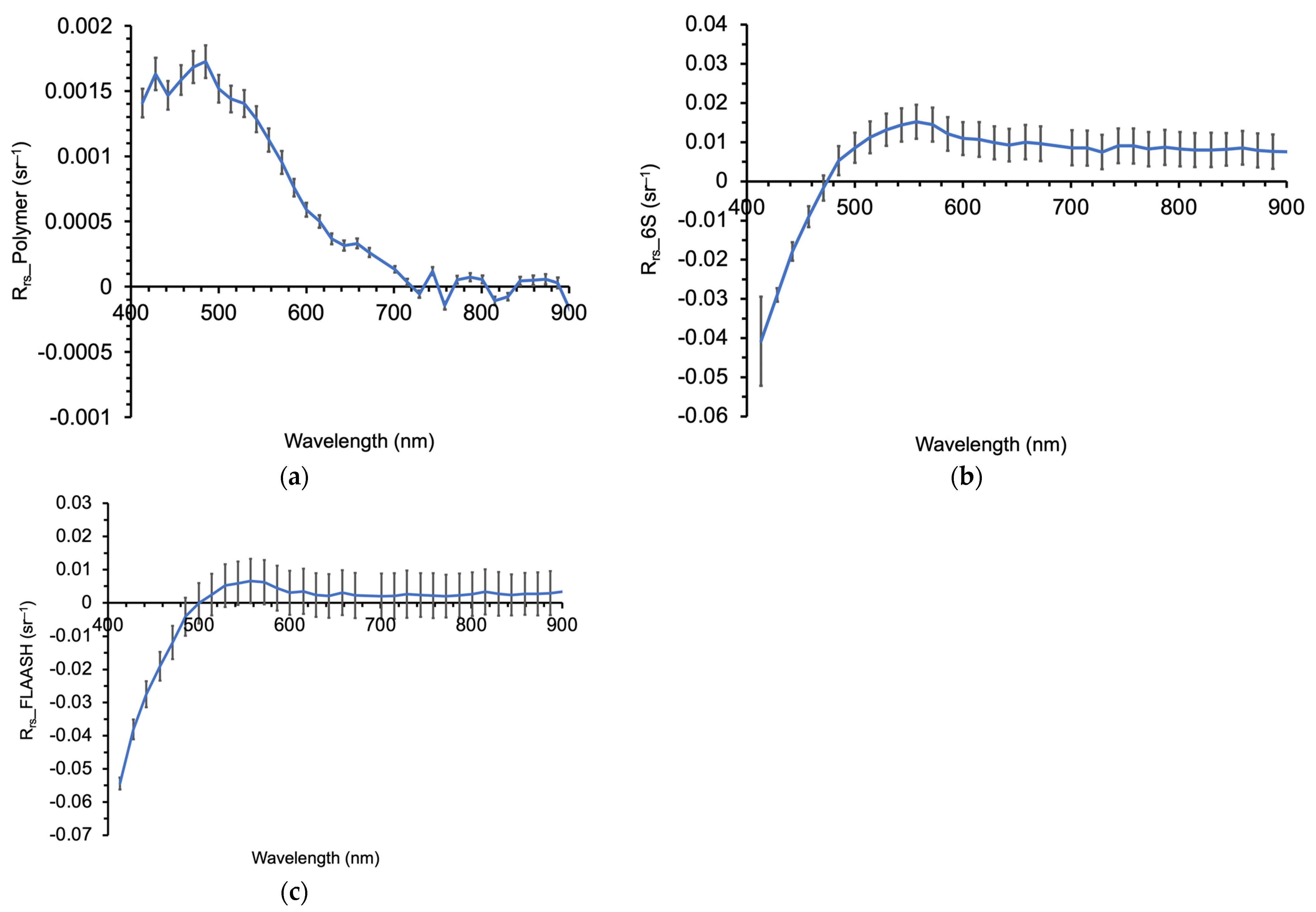
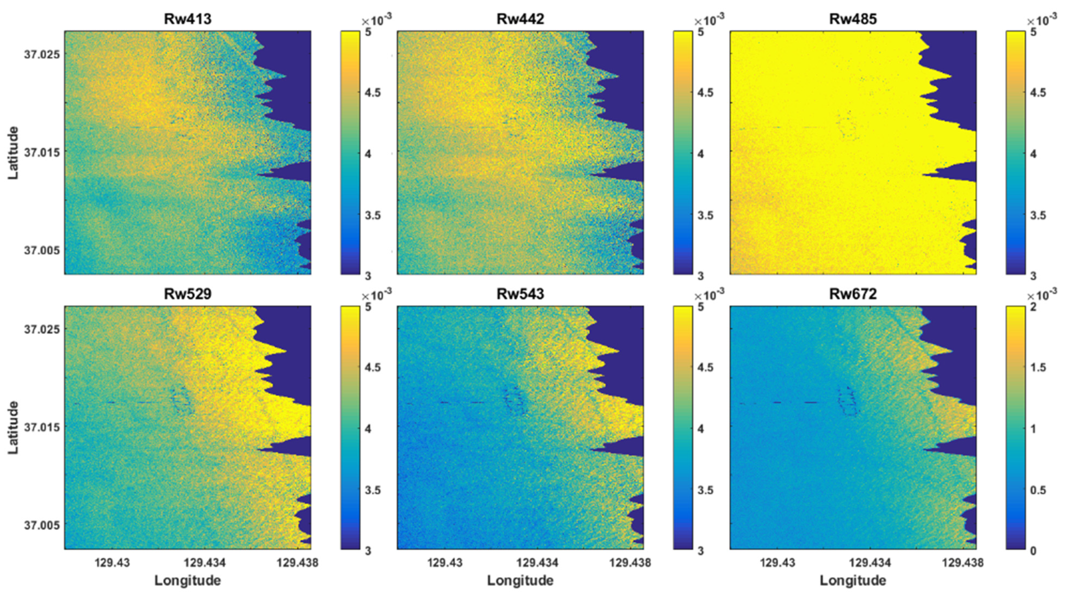
3.2. Polymer, 6S, and FLAASH Results for CASI-1500

To compare the atmospheric correction approaches, the entire CASI-1500 radiance imagery (Figure 1a) was corrected using Polymer, 6S, and FLAASH, after which Rrs data were extracted from 57 pixels, i.e., the red symbols in Figure 1a. All Rrs spectra from the 57 pixels were averaged and plotted with error bars of one standard deviation (Figure 3). The Rrs spectra from wavelengths above 900 nm are not shown because the CASI-1500 data were usually unstable and not informative in that wavelength range.
The spectral shape of Rrs after applying the Polymer algorithm (Figure 3a) was generally consistent with that of CASI-1500 radiance and apparent reflectance (Figure 2), but the magnitude of Rrs was smaller at all spectral bands. In contrast, although Rrs from both 6S and FLAASH (Figure 3b,c) had similar spectral shape and magnitude, they differed greatly from Rrs obtained using Polymer both in spectral shape and magnitude. In addition, Rrs using 6S and FLAASH were negative in the blue bands (400–500 nm) and higher than apparent reflectance values in other bands.
CASI Rrs values using 6S and FLAASH were overcorrected in the blue bands. This was probably caused by inaccurate input parameters, particularly the atmospheric parameters. Therefore, we examined a variation of CASI Rrs with aot_550 and water vapour for 6S (Figure 4a,b) and visibility for FLAASH (Figure 4c) at a test point (129.435°E, 36.985°N). For 6S atmospheric correction, the referenced aot_550 and water vapour values were 0.316 and 1.64 cm, respectively; for FLAASH atmospheric correction, the referenced visibility value was 14.85 km. The other two atmospheric values in each plot were 0.5 times and 1.5 times of the referenced value, respectively.
For 6S atmospheric correction, the magnitude of the entire Rrs spectrum increased and decreased significantly with the decrease and increase in aot_550 (Figure 4a), respectively, whereas the magnitude of Rrs changed little with variation of water vapour. Similarly, for FLAASH atmospheric correction, the magnitude of the entire Rrs spectrum increased significantly with the increase in visibility.

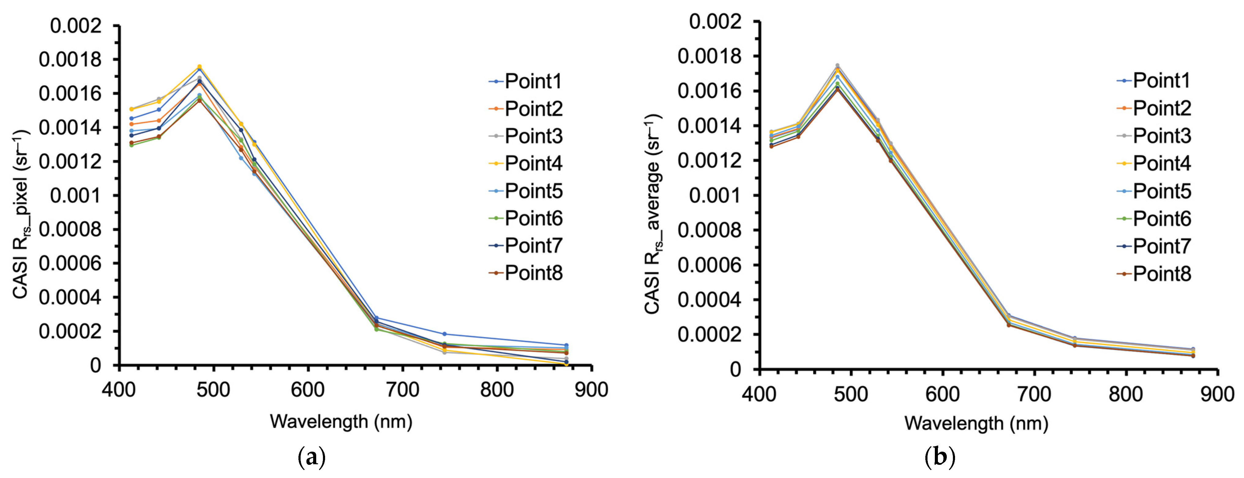
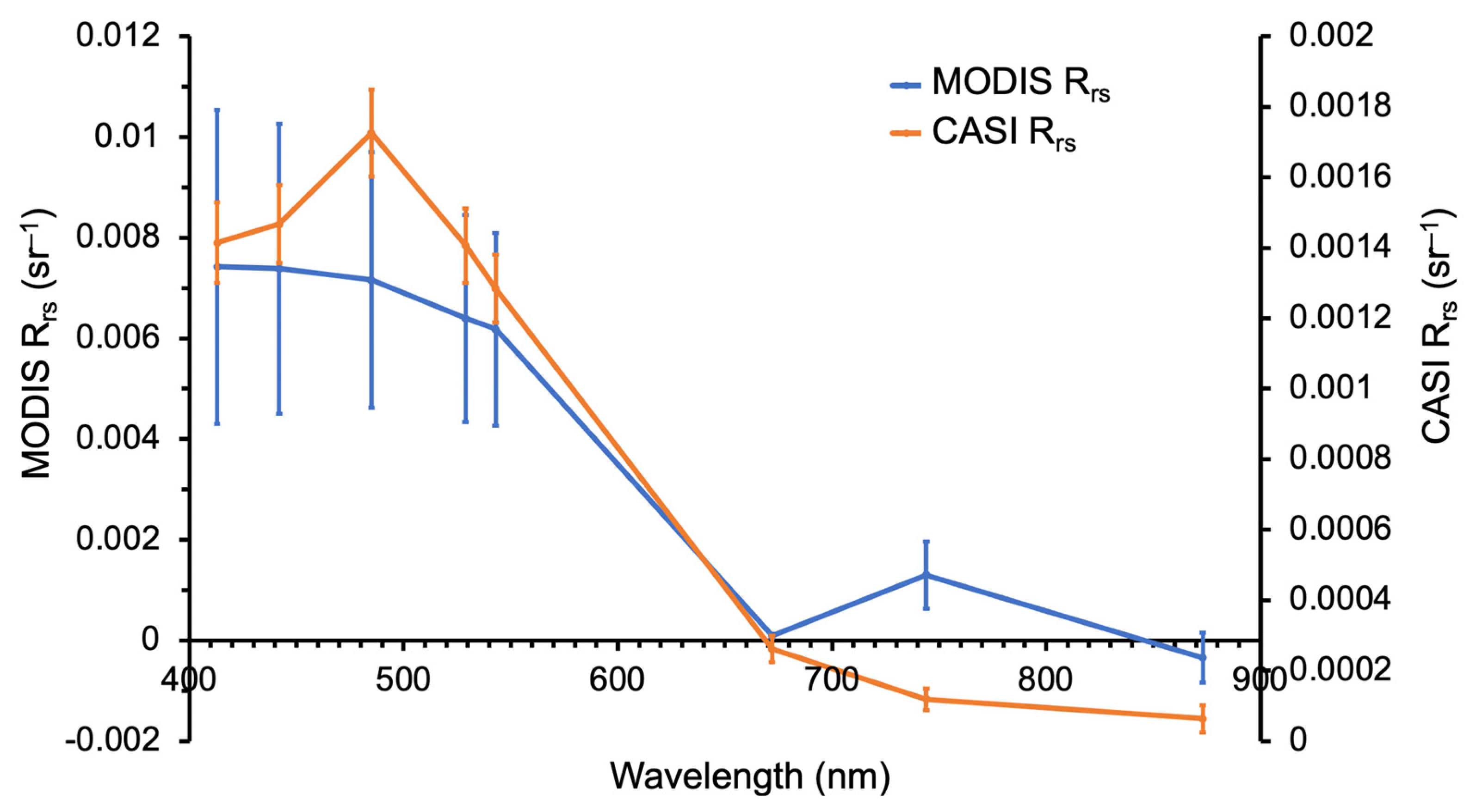
3.3. Comparison of the Polymer Results for CASI-1500 and MODIS

Previously, Zhang et al. [22] applied Polymer to MODIS data and compared its performance with in situ Rrs to conclude that it did not perform better than the standard NASA atmospheric correction algorithm (traditional near-infrared (NIR) approach [37]), at blue bands but was comparable at green and red bands. Therefore, they proposed using Polymer as a surrogate for the NASA NIR approach when MODIS Rrs data were limited.
In this study, due to lack of in situ Rrs data, we evaluated the performance of Polymer by comparing the Rrs results from CASI-1500 and MODIS. MODIS bands selected were 412, 443, 488, 531, 547, 667, 748, and 869 nm, and the corresponding CASI-1500 bands were 413, 442, 485, 529, 543, 672, 744, and 873 nm. Regarding the different pixel resolution of the two sensors, spatial distribution of CASI Rw (water-leaving reflectance) using Polymer was examined. As the data volume of whole CASI radiance image (Figure 1) was too big to process at one time, the image was divided into eight parts. Images of CASI Rw at 413, 442, 485, 529, 543, and 672 nm were made for one part of the whole area (129.428°–129.438°E, 37.002°–37.027°N) (Figure 5).
Spatial variability of Rw at each band was observed. To quantify the variability, pixel and averaged Rrs were compared for eight points (No. 4, No. 5, No. 6, No. 7, No. 8, No. 9, No. 10, and No. 11) in each Rw image (Figure 6). In general, the pixel and averaged CASI Rrs showed similar spectral shape and magnitude for each point. Therefore, pixel CASI Rrs was compared with pixel MODIS Rrs for simplifying data processing (Figure 7).
Despite being measured on different days, Rrs spectra from CASI-1500 and MODIS generally matched except for inconsistencies at 485 and 744 nm. In addition, across the entire spectrum, MODIS Rrs values were much higher than CASI-1500 Rrs values. At 488 nm for instance, MODIS Rrs was approximately 0.007 sr−1, whereas the CASI-1500 Rrs at 485 nm was 0.002 sr−1.
The correlation between the CASI-1500 and MODIS Rrs spectra (Figure 8) was statistically significant (R2 = 0.98), but the slope (0.21) was low, suggesting that the CASI-1500 Rrs were generally 0.8 times lower than MODIS Rrs. We further calculated the cosine distance between the two spectra and the cos(α) was approximately 0.99, which suggested that the two spectra were closely matched.

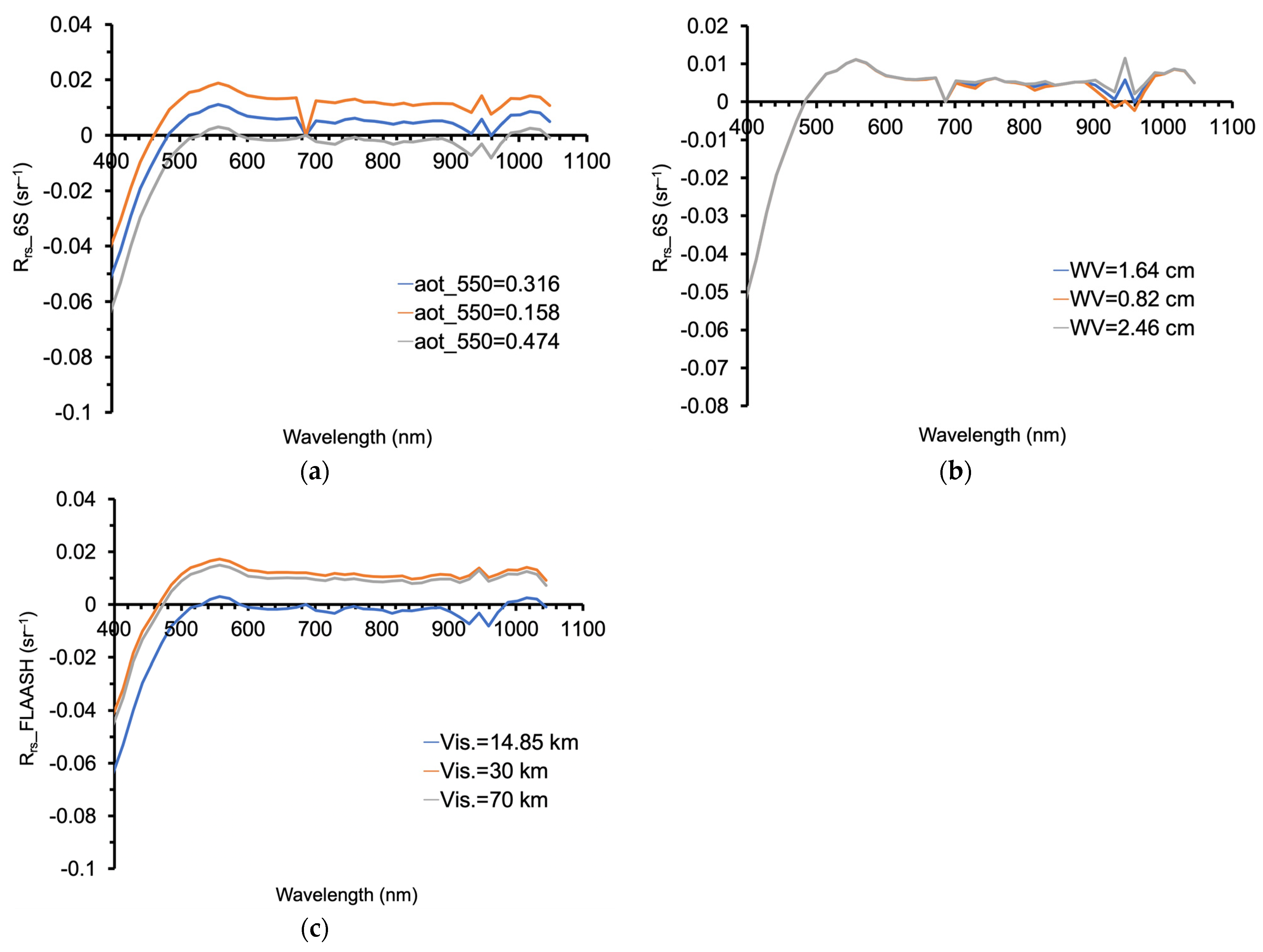
3.4. Variation of Polymer Results with Aerosol and Water Vapor for CASI-1500

For understanding the discrepancy between CASI-1500 and MODIS Rrs at each band, the variation in CASI-1500 Rrs with aot_550 and water vapour was investigated (Figure 9). The processing of CASI-1500 radiance data (as described in Section 2.3) was undertaken again with various aot_550 values, including 0, 0.01, 0.05, 0.1, 0.2, 0.3, and 0.4, and various water vapour values, including 0, 1, 1.5, 2, 3, and 4 cm, for the 6S input. The Rrs spectra obtained by applying Polymer to CASI-1500 Rrs for test locations showed that variation in CASI-1500 derived Rrs spectra due to aerosols and water vapour was small.

4. Discussion

4.1. Comparison among Polymer, 6S, and FLAASH

In this study, we applied Polymer to airborne hyperspectral CASI-1500 data and compared the resulting Rrs to two other widely used atmospheric correction approaches, i.e., 6S and FLAASH. The spectral shape of CASI-1500 Rrs using Polymer (Figure 3a) was similar to that of CASI-1500 apparent reflectance (Figure 2b), suggesting that the atmospheric effects influencing CASI-1500 radiance data on the acquisition day might be small. Moreover, the spectral shapes of CASI-1500 Rrs and MODIS Rrs using Polymer were highly correlated statistically, suggesting that the Rrs derived using Polymer were accurate.
In contrast, both 6S and FLAASH underestimated CASI-1500 Rrs, with negative values in the blue bands (400–500 nm). The Rrs values at other wavelengths were even larger than the CASI-1500 apparent reflectances, a clear indication that these two atmospheric correction approaches were estimating Rrs erroneously. Therefore, we conclude that the performance of Polymer is better than the performance of 6S and FLAASH. Despite the superior performance of Polymer, rigorous validation with in situ Rrs is necessary, which we plan to carry out when in situ Rrs data become available.
Polymer was originally designed to retrieve ocean colour in the presence of sun glint using MERIS data. The author concluded that Polymer greatly increased the spatial coverage of MERIS measurements for ocean colour and that the accuracy of retrieved data was not significantly reduced in high glint areas and remained the same as the standard algorithm outside sun glint areas [14]. The performance of Polymer was further evaluated by applying it to other satellite sensors. A recent study [22] compared Polymer with the traditional near-infrared (NIR) approach for MODIS-Aqua data and reported that Polymer did not perform better at blue bands but was comparable at green and red bands. Therefore, MODIS Rrs from Polymer was considered as reliable, at least not worse. The performance of Polymer to CASI data was then evaluated by comparing CASI Rrs with MODIS Rrs. However, CASI and MODIS Rrs showed big difference in their magnitude though their spectral shapes were similar. One possible cause for this difference may be errors in the MODIS Rrs.
Several studies [19,20] have compared Rrs after application of 6S and FLAASH to medium and high-resolution data. Recently, Eugenio et al. [18] applied 6S and FLAASH to WorldView-2 high-resolution satellite data and validated the atmospheric correction results with fields above water Rrs. They reported that both approaches achieved excellent results, although 6S produced slightly superior results. Our sub-optimal results using 6S and FLAASH for CASI-1500 hyperspectral imagery could be because the atmospheric products used were not accurate and the algorithms did not apply to these waters. In the future, to obtain more realistic atmospheric products, we need to consider two approaches. One is to make field measurements during CASI-1500 overflights, and the other is to develop algorithms to retrieve atmospheric products from CASI-1500 data.

4.2. Discrepancy of the CASI-1500 and MODIS Rrs with Polymer

The magnitude of CASI-1500 Rrs was approximately 0.8 times lower than that of MODIS Rrs (Figure 8). The possible reasons include: (1) dfference in the acquisition time of CASI-1500 versus MODIS data, the CASI-1500 data used was one day later than the MODIS data; (2) MODIS pixel size (1 km × 1 km) is much coarser than that of CASI-1500 (1 m × 1 m); (3) atmospheric products, such as MODIS water vapour and reanalysis aot_550, were also of much coarser spatial resolution than CASI-1500 data, which might affect the 6S output parameters and thus the atmospheric correction of CASI-1500 data with Polymer; (4) satellite measurements of coastal waters near land/water surfaces suffer from land adjacency effects [38], thus the MODIS 1 km pixels will most likely be affected by the adjacency and contamination of land signals much more than the low altitude and high resolution CASI data; and (5) errors in MODIS Rrs from Polymer. However, as we investigated the pixel CASI Rrs and averaged CASI Rrs within MODIS 1 km pixel were similar in spectral shape and magnitude, and the variation in Rrs using Polymer and CASI-1500 data with various values of aot_550 and water vapour and found them to be very small (Figure 6), we conclude that the discrepancies in Rrs between CASI-1500 and MODIS Rrs may be due to (1), (4), and (5).

5. Conclusions

Atmospheric correction may be required before application of airborne hyperspectral data analysis. The traditional atmospheric correction approach for CASI data has been FLAASH. However, the performance of FLAASH depends on the accuracy of input atmospheric parameters, including aerosol, water vapour, and ozone, which are often unavailable during the acquisition of airborne data.
Therefore, in this study, we evaluated three of the most widely used atmospheric correction approaches, i.e., Polymer, 6S, and FLAASH, and take the position that Polymer was the most suitable for application to CASI-1500 data. We further evaluated Polymer by comparing the Rrs derived from CASI-1500 and MODIS after using this atmospheric correction. Spectral shapes of Rrs from both sensors correlated significantly, although the magnitude of CASI-1500 Rrs was much lower than that of MODIS Rrs. We ascribe this difference to the one day difference in data acquisition between the two sensors, higher land adjacency effect for MODIS than for CASI-1500, and possible errors in MODIS Rrs from Polymer.
Our future plans include collecting in situ Rrs data to validate Rrs from CASI-1500 after application of the Polymer atmospheric correction, after which we will continue to modify the Polymer algorithm to improve its atmospheric correction and ocean reflectance models. In case of the atmospheric correction model, we plan to remove or reduce the effect of sky radiance, whereas for the ocean reflectance model, we plan to address the bottom reflectance effect in shallow waters.

Author Contributions

Conceptualization, M.Y. and W.K.; methodology, M.Y. and W.K.; software, M.Y., Y.H., F.A.K. and H.T.; validation, M.Y.; formal analysis, M.Y.; investigation, M.Y.; resources, W.K.; data curation, M.Y. and W.K.; writing—original draft preparation, M.Y.; writing—review and editing, M.Y., W.K., Y.H., H.T., F.A.K., Q.L., J.I.G. and H.d.R.G.; visualization, M.Y.; supervision, W.K.; project administration, W.K.; funding acquisition, W.K. All authors have read and agreed to the published version of the manuscript.

Funding

This research was supported by (1) basic research program through the National Research Foundation of Korea (NRF) funded by the Ministry of Science, ICT and Future Planning, grant number: NRF-2019R1F1A1062585.

Institutional Review Board Statement

Not applicable.

Informed Consent Statement

Not applicable.

Acknowledgments

We are thankful to the NRF and FIRA for providing the funding and to the Ocean Ecology Laboratory and Ocean Biology Processing Group of NASA Goddard Space Flight Center for providing daily Moderate-resolution Imaging Spectroradiometer (MODIS) Aqua L2 data, MODIS atmospheric products (MYD04, MYD05, and MYDO7), and reanalysis MERRA-2 data of Total Aerosol Extinction AOT [550 nm] (TOTEXTTAU), 2-m eastward wind (U2M), and 2-m northward wind (V2M). We are also thankful to the Korea Fisheries Resources Agency (FIRA) funded by the Ministry of Oceans and Fisheries, Republic of Korea. JIG and HRG are supported by NASA 80LARC21DA002-GLIMR AABO8078 and NOAA GST SA18-CUNY01.

Conflicts of Interest

The authors declare no conflict of interest. The funders had no role in the design of the study; in the collection, analyses, or interpretation of data; in the writing of the manuscript, or in the decision to publish the results.

References

  1. Moses, W.J.; Gitelson, A.A.; Perk, R.L.; Gurlin, D.; Rundquist, D.C.; Leavitt, B.C.; Barrow, T.M.; Brakhage, P. Estimation of chlorophyll-a concentration in turbid productive waters using airborne hyperspectral data. Water Res. 2012, 46, 993–1004. [Google Scholar] [CrossRef] [Green Version]
  2. Gould, R.W., Jr.; Arnone, R.A. Remote sensing estimates of inherent optical properties in a coastal environment. Remote Sens. Environ. 1997, 61, 290–301. [Google Scholar] [CrossRef]
  3. Kallio, K.; Kutser, T.; Hannonen, T.; Koponen, S.; Pulliainen, J.; Vepsaälaäinen, J.; Pyhaälahti, T. Retrieval of water quality from airborne imaging spectrometry of various lake types in different seasons. Sci. Total Environ. 2001, 268, 59–77. [Google Scholar] [CrossRef]
  4. Ibrahim, A.; Franz, B.; Ahmad, Z.; Healy, R.; Knobelspiesse, K.; Gao, B.; Proctor, C.; Zhai, P.-W. Atmospheric correction for hyperspectral ocean color retrieval with application to the Hyperspectral Imager for the Coastal Ocean (HICO). Remote Sens. Environ. 2018, 204, 60–75. [Google Scholar] [CrossRef] [Green Version]
  5. Gao, B.C.; Montes, M.J.; Davis, C.O.; Goetz, A.F.H. Atmospheric correction algorithms for hyperspectral remote sensing data of land and ocean. Remote Sens. Environ. 2009, 113, S17–S24. [Google Scholar] [CrossRef]
  6. Gao, B.C.; Davis Curtiss, O.; Goetz, A.F.H. A review of atmospheric correction techniques for hyperspectral remote sensing of land surfaces and ocean colour. In Proceedings of the 2006 IEEE International Symposium on Geoscience and Remote Sensing, Denver, CO, USA, 31 July–4 August 2006; pp. 1979–1981. [Google Scholar]
  7. Gao, B.-C.; Montes, M.J.; Ahmad, Z.; Davis, C.O. Atmospheric correction algorithm for hyperspectral remote sensing of ocean color from space. Appl. Opt. 2000, 39, 887–896. [Google Scholar] [CrossRef] [PubMed] [Green Version]
  8. Qu, Z.; Goetz, A.F.H.; Heidebrecht, K.B. High accuracy atmospheric correction for hyperspectral data (HATCH). In Proceedings of the Ninth JPL Airborne Earth Science Workshop, 23–25 February 2000; Green, R.O., Ed.; Jet Propulsion Laboratory: Pasadena, CA, USA, 2000. [Google Scholar]
  9. Gao, B.-C.; Heidebrecht, K.H.; Goetz, A.F.H. Derivation of scaled surface reflectances from AVIRIS data. Remote Sens. Environ. 1993, 44, 165–178. [Google Scholar] [CrossRef]
  10. Kruse, F.A. Use of airborne imaging spectrometer data to map minerals associated with hydrothermally altered rocks in the northern Grapevine Mountains, Nevada and California. Remote Sens. Environ. 1988, 24, 31–51. [Google Scholar] [CrossRef]
  11. Clark, R.N.; King, T.V.V. Causes of spurious features in spectral reflectance data. In Proceedings of the 3rd Airborne Imaging Spectrometer Data Analysis Workshop; Vane, G., Ed.; Jet Propulsion Laboratory: Pasadena, CA, USA, 1987; pp. 49–61. [Google Scholar]
  12. Conel, J.E.; Green, R.O.; Vane, G.; Bruegge, C.J.; Alley, R.E. AIS-2 radiometry and a comparison of methods for the recovery of ground reflectance. In Proceedings of the 3rd Airborne Imaging Spectrometer Data Analysis Workshop; Vane, G., Ed.; Jet Propulsion Laboratory: Pasadena, CA, USA, 1987; pp. 18–47. [Google Scholar]
  13. Roberts, D.A.; Yamaguchi, Y.; Lyon, R. Comparison of various techniques for calibration of AIS data. In Proceedings of the 2nd Airborne Imaging Spectrometer Data Analysis Workshop; Vane, G., Goetz, A.F.H., Eds.; Jet Propulsion Laboratory: Pasadena, CA, USA, 1986; pp. 21–30. [Google Scholar]
  14. Steinmetz, F.; Deschamps, P.-Y.; Ramon, D. Atmospheric correction in presence of sun glint: Application to MERIS. Opt. Express 2011, 19, 9783–9800. [Google Scholar] [CrossRef] [Green Version]
  15. Pu, R.; Landry, S.; Zhang, J. Evaluation of Atmospheric Correction Methods in Identifying Urban Tree Species with WorldView-2 Imagery. IEEE J. Sel. Top. Appl. Earth Obs. Remote Sens. 2015, 8, 1886–1897. [Google Scholar] [CrossRef]
  16. Vanonckelen, S.; Lhermitte, S.; Van Rompaey, A. The effect of atmospheric and topographic correction methods on land cover classification accuracy. Int. J. Appl. Earth Obs. Geoinf. 2013, 24, 9–21. [Google Scholar] [CrossRef] [Green Version]
  17. El Hajj, M.; Bégué, A.; Lafrance, B.; Hagolle, O.; Dedieu, G.; Rumeau, M. Relative Radiometric Normalization and Atmospheric Correction of a SPOT 5 Time Series. Sensors 2008, 8, 2774–2791. [Google Scholar] [CrossRef] [PubMed] [Green Version]
  18. Eugenio, F.; Marcello, J.; Martin, J.; Esparragón, D.R. Benthic habitat mapping using multispectral high-resolution imagery: Evaluation of shallow water atmospheric correction techniques. Sensors 2017, 17, 2639. [Google Scholar] [CrossRef] [PubMed] [Green Version]
  19. Marcello, J.; Eugenio, F.; Perdomo, U.; Medina, A. Assessment of Atmospheric Algorithms to Retrieve Vegetation in Natural Protected Areas Using Multispectral High-resolution Imagery. Sensors 2016, 16, 1624. [Google Scholar] [CrossRef] [Green Version]
  20. Nguyen, H.C.; Jung, J.; Lee, J.; Choi, S.U.; Hong, S.Y.; Heo, J. Optimal Atmospheric Correction for Above-Ground Forest Biomass Estimation with the ETM+ Remote Sensor. Sensors 2015, 15, 18865–18886. [Google Scholar] [CrossRef] [Green Version]
  21. Steinmetz, F.; Ramon, D. Sentinel-2 MSI and Sentinel-3 OLCI consistent ocean colour products using POLYMER. In Remote Sensing of the Open and Coastal Ocean and Inland Waters; International Society for Optics and Photonics: Bellingham, WA, USA, 2018; p. 107780E. [Google Scholar]
  22. Zhang, M.; Hu, C.; Cannizzaro, J.; English, D.; Barnes, B.B.; Carlson, P.; Yarbro, L. Comparison of two atmospheric correction approaches applied to MODIS measurements over north American waters. Remote Sens. Environ. 2018, 216, 442–455. [Google Scholar] [CrossRef]
  23. Wang, J.W.; Lee, Z.P.; Wei, J.W.; Du, K.P. A Scheme of Atmospheric Correction with A Revised POLYMER model Using Same-day Observations. Opt. Express 2020, 28, 26953–26976. [Google Scholar] [CrossRef]
  24. Vermote, E.; Tanré, D.; Deuzé, J.; Herman, M.; Morcrette, J.; Kotchenova, S. Second simulation of a satellite signal in the solar spectrum-vector (6SV) 6S User Guide Version 3. In Remote Sensing: Models and Methods for Image Processing; Schowengerdt, R.A., Ed.; Academic Press: Cambridge, MA, USA, 2006. [Google Scholar]
  25. Kotchenova, S.Y.; Vermote, E.F. Validation of a vector version of the 6S radiative transfer code for atmospheric correction of satellite data, Part II: Homogeneous Lambertian and anisotropic surfaces. Appl. Opt. 2007, 46, 4455–4464. [Google Scholar] [CrossRef] [Green Version]
  26. Kotchenova, S.Y.; Vermote, E.F.; Matarrese, R.; Klemm, F.J., Jr. Validation of a vector version of the 6S radiative transfer code for atmospheric correction of satellite data, Part I: Path radiance. Appl. Opt. 2006, 45, 6762–6774. [Google Scholar] [CrossRef] [Green Version]
  27. Hu, Y.; Liu, L.Y.; Liu, L.L.; Peng, D.L.; Jiao, Q.J.; Zhang, H. A Landsat-5 atmospheric correction based on MODIS atmosphere products and 6S model. IEEE J. Sel. Top. Appl. Earth Obs. Remote Sens. 2014, 7, 1609–1615. [Google Scholar] [CrossRef]
  28. Kruse, F.A. Comparison of ATREM, ACORN, and FLAASH atmospheric corrections using low-altitude AVIRIS data of Boulder, Colorado. In Proceedings of the 13th JPL Airborne Geosci. Workshop; International Society for Optics and Photonics: Pasadena, CA, USA, 2004. [Google Scholar]
  29. Hu, C.; Carder, K. Atmospheric correction for airborne sensors: Comment on a scheme used for CASI. Remote Sens. Environ. 2002, 79, 134–137. [Google Scholar] [CrossRef]
  30. Adler-Golden, S.; Berk, A.; Bernstein, L.S.; Richtsmeier, S.; Acharya, P.K.; Matthew, M.W.; Anderson, G.P.; Allred, C.L.; Jeong, L.S.; Chetwynd, J.H. FLAASH, a modtran4 atmospheric correction package for hyperspectral data retrievals and simulations. In Proceedings of the 7th JPL Airborne Earth Sci Workshop, Pasadena, CA, USA, 12–16 January 1998; Jet Propulsion Laboratory: Pasadena, CA, USA, 1998. [Google Scholar]
  31. Kim, W.; Kim, S.H.; Baek, S.; Kim, H.; Oh, J. A Preliminary Study on Benthic Mapping of Uljin Coast Based on Airborne Hyperspectral Imagery Towards the Whitening Detection. J. Coast. Res. 2020, 114, 464–468. [Google Scholar] [CrossRef]
  32. Cox, C.; Munk, W. Measurement of the roughness of the sea surface from photographs of the sun’s glitter. J. Opt. Soc. Am. 1954, 44, 838–850. [Google Scholar] [CrossRef]
  33. Wang, M.; Bailey, S.W. Correction of sun glint contamination on the SeaWiFS ocean and atmosphere products. Appl. Opt. 2001, 40, 4790–4798. [Google Scholar] [CrossRef]
  34. Cooley, T.; Anderson, G.P.; Felde, G.W.; Hoke, M.L.; Ratkowski, A.J.; Chetwynd, J.H.; Gardner, J.A.; Adler-Golden, S.M.; Matthew, M.W.; Berk, A. FLAASH, a MODTRAN4-based atmospheric correction algorithm, its application and validation. IEEE Int. Geosci. Remote Sens. Symp. 2002, 3, 1414–1418. [Google Scholar]
  35. Schowengerdt, R.A. Remote Sensing: Models and Methods for Image Processing; Academic Press: Cambridge, MA, USA, 2006. [Google Scholar]
  36. Wei, J.; Lee, Z.-P.; Shang, S. A system to measure the data quality of spectral remote sensing reflectance of aquatic environments. J. Geophys. Res. Ocean. 2016, 121, 8189–8207. [Google Scholar] [CrossRef]
  37. Gordon, H.R.; Wang, M. Retrieval of water-leaving radiance and aerosol optical thickness over the oceans with SeaWiFS: A preliminary algorithm. Appl. Opt. 1994, 33, 443–452. [Google Scholar] [CrossRef]
  38. Feng, L.; Hu, C. Land adjacency effects on MODIS Aqua top-of-atmosphere radiance in the shortwave infrared: Statistical assessment and correction. J. Geophys. Res. Ocean. 2017, 122, 4802–4818. [Google Scholar] [CrossRef]
Figure 1. Location of Uljin coast, Korea: (a) red symbols represent locations where CASI data were processed using Polymer, 6S, and FLAASH, and green symbols denote locations where MODIS data processed by Polymer were extracted; (b) water depth of the coastal waters with labelled contour lines.
Remotesensing 13 05062 g001
Figure 2. (a) CASI-1500 radiance data; (b) the calculated apparent reflectance data. The data were acquired on 4 May 2019 over the Uljin coast. Point1′ to Point8′ (Nos. 1, 9, 17, 25, 33, 41, 49, and 57) correspond from top to bottom to the evenly distributed line of red symbols in Figure 1.
Remotesensing 13 05062 g002
Figure 3. Averaged Rrs spectra from CASI-1500 atmospherically corrected using Polymer (a), 6S (b), FLAASH (c). The error bars in each plot represent one standard deviation.
Remotesensing 13 05062 g003
Figure 4. CASI-1500 Rrs spectra at various aot_550 values (a) and various water vapour values (b) after application of the 6S atmospheric correction, and at various visibility values (c) after application of the FLAASH atmospheric correction.
Remotesensing 13 05062 g004
Figure 5. CASI-1500 Rw images at 413, 442, 485, 529, 543, and 672 nm.
Remotesensing 13 05062 g005
Figure 6. Comparison of pixel (a) and averaged (b) CASI-1500 Rw spectra after applying the Polymer atmospheric correction.
Remotesensing 13 05062 g006
Figure 7. Comparison of averaged CASI-1500 and MODIS Rrs spectra after applying the Polymer atmospheric corrected algorithm. CASI-1500 and MODIS Rrs were averaged for Rrs from all locations denoted by red and green symbols in Figure 1a, respectively. The error bars represent one standard deviation.
Remotesensing 13 05062 g007
Figure 8. Scatter plot of the averaged CASI-1500 Rrs at bands 413, 442, 485, 529, 543, 672, 744, and 873 nm versus the averaged MODIS Rrs at bands 412, 443, 488, 531, 547, 667, 748, and 869 nm; N represents the data number for each band.
Remotesensing 13 05062 g008
Figure 9. CASI-1500 Rrs spectra at various aot_550 values (a) and various water vapour values (b) after application of the Polymer atmospheric correction.
Remotesensing 13 05062 g009
Table 1. Spectral bands and width of the CASI-1500 sensor for data acquired on 4 May 2019.
Band
Number
Center Wavelength
(nm)
Band
Number
Center Wavelength
(nm)
Band
Number
Center Wavelength
(nm)
Band
Number
Center Wavelength
(nm)
Full Width at
Half Maximum (nm)
1370.213542.825715.137887.17.2
2384.614557.226729.438901.5
339915571.527743.739915.8
4413.416585.928758.140930.2
5427.817600.329772.441944.5
6442.218614.630786.842958.8
7456.619629.031801.143973.2
847120643.332815.444987.5
9485.321657.733829.8451001.9
10499.722672.034844.1461016.2
11514.123686.435858.5471030.6
12528.524700.736872.8481044.9
Table 2. Description of the 6S input parameters for CASI-1500 data collected on 4 May 2019.
ParametersData SourceSpatial ResolutionTemporal ResolutionValue
Solar zenith angle33.663°
Solar azimuth angle239.218°
Sensor zenith angleBy pixel
Sensor azimuth angle270°
Total water vapourMYD051 km × 1 kmDaily1.77 cm
Total ozoneMYD071 km × 1 kmDaily0.34 cm-atm
Aerosol modelMaritime
aot_550MERRA-20.5° × 0.625°Hourly0.32
Wind speedMERRA-20.5° × 0.625°Hourly1.91 m s−1
Wind azimuth angle313.004°
Chl-a concentrationMODIS-Aqua Level-21 km × 1 kmDaily3.76 mg m−3
Sea water salinity 34.3 ppt
Table 3. Description of the FLAASH input parameters applied to CASI-1500 data collected on 4 May 2019.
ParameterValue
Image center location37.05057344°N,
129.41963701°E.
Sensor altitude2 km
Ground elevation0.01 km
Pixel size1 m
Flight date4-May-19
Flight time GMT5:17:47
Atmospheric modelMid-Latitude Summer
Aerosol modelMaritime
Aerosol retrievalNone
Initial visibility14.85 km
Water retrievalYes
Water absorption feature940 nm
Modtran resolution5 cm−1
Modtran multiscatter modelScaled DISORT
DISCORT streams number8
Publisher’s Note: MDPI stays neutral with regard to jurisdictional claims in published maps and institutional affiliations.

