Automated Building Detection from Airborne LiDAR and Very High-Resolution Aerial Imagery with Deep Neural Network

Abstract

The detection of buildings in the city is essential in several geospatial domains and for decision-making regarding intelligence for city planning, tax collection, project management, revenue generation, and smart cities, among other areas. In the past, the classical approach used for building detection was by using the imagery and it entailed human–computer interaction, which was a daunting proposition. To tackle this task, a novel network based on an end-to-end deep learning framework is proposed to detect and classify buildings features. The proposed CNN has three parallel stream channels: the first is the high-resolution aerial imagery, while the second stream is the digital surface model (DSM). The third was fixed on extracting deep features using the fusion of channel one and channel two, respectively. Furthermore, the channel has eight group convolution blocks of 2D convolution with three max-pooling layers. The proposed model’s efficiency and dependability were tested on three different categories of complex urban building structures in the study area. Then, morphological operations were applied to the extracted building footprints to increase the uniformity of the building boundaries and produce improved building perimeters. Thus, our approach bridges a significant gap in detecting building objects in diverse environments; the overall accuracy (OA) and kappa coefficient of the proposed method are greater than 80% and 0.605, respectively. The findings support the proposed framework and methodologies’ efficacy and effectiveness at extracting buildings from complex environments.

1. Introduction

The numerical growth of the population in urban centers through the migration of the population from rural to urban areas is a defining feature of today’s society. Humans continue to move to major cities from rural regions, pushing for accelerated urban growth, leading to high demand for living space and working space, and increasing the potential for precise, accurate, and up-to-date 3D city models. The production of such models is still a challenging task. In this context, generating automatic and accurate building maps as quickly as possible and with excellent accuracy of results is an increasingly stringent requirement taken into account by local public authorities and decision-makers. The results thus obtained have many uses, among which is the need for integrated and responsible planning of the city following the principles of sustainable development [1,2,3,4,5]. Hence, the condition of urban buildings remains a crucial research topic in computer vision and image processing technology [6]. A vast amount of energy is expended on the specialists’ interpretation and detection of features in photogrammetry imagery. However, it is inefficient and costly to discriminate buildings from other features and define their outline manually. As a result, many buildings detection approaches have been documented throughout the past several centuries [7,8,9].

Nevertheless, achieving one hundred percent accurate automatic building detection remains a pipe dream. There have been various explanations for this circumstance. The complex morphology of urban areas is a challenge to describe the shape of buildings and infrastructures accurately. In contrast, others have low-density structures, challenging scenes or uneven terrain, acquisition angles, shadows, and occlusions incidence. Furthermore, buildings and other comparable objects in an urban setting have similar spectral and spatial physiognomies [10,11]. Thanks to new technologies, different sensors such as satellite imagery, high-resolution aerial imagery, radar (radio detection and ranging), and even laser scanning sensors can be an excellent possibility for a solution [12]. Among the sensors mentioned above, one of the newest technologies that have transformed buildings’ detection and extraction is the airborne light detection and ranging (LiDAR) sensor. This innovative technology helps to improve urban building detection problems and is also valuable for informed decisions. LiDAR is widely referred to as laser scanners.

The airborne LiDAR sensor has a tremendous impact on city mapping, high accuracy, extensive area coverage, fast acquisition, and it provides an efficient and accurate building footprint because of its high-density point cloud, short data capture period, and good vertical accuracy, with high-density 3D point clouds for ground object collection [13,14]. The fundamental merit of LiDAR over the photogrammetric technique is its capability to penetrate depth based on height information [15,16]. In contrast, photogrammetry datasets generate massive data volumes that may necessitate parallel processing and, as a result, a putting fortune in computer hardware to quickly and efficiently process, distribute, and share. As a result of integrating many data sources, the accuracy and reliability of the extraction outcomes improve [17]. Hence, it leads to refinement and robustness of the extraction outputs. Thus, in recent times, advanced practices employ fusing data sources for building extraction from more sensors rather than adopting a single data source [18,19].

Conventionally, machine learning paradigms exploits “shallows” architectures; they initially alter acquired raw data into a multidimensional feature space and then optimally approximate linear or even nonlinear associations [20]. Consequently, machine learning is a suitable tool for the efficiency and robustness of the necessary forms of artificial intelligence algorithms. The deep learning methods are robust for several real-world fields such as image classification, detection, extraction, reconstruction, computer vision, and others [17]. It is possible to automatically extract outlines via machine learning approaches by building a deep neural network. Convolutional neural networks (CNN) are widely used for deep learning and are specifically suitable for image detection, extraction, and modelling. They vary from other neural networks in little ways: a visual cortex’s biologic Ral structure inspires CNNs and contains complex and straightforward cells [21]. These cells help to activate the sub-regions of a visual field.

These sub-regions are named receptive fields. The neurons in a convolutional layer link to the layers’ sub-regions before that layer as a substitute for being fully connected as in other forms of neural networks. The neurons are unresponsive to the areas outside of these sub-regions in the image. These sub-regions will cross paths. As a result, the neurons of CNN’s generate spatially associated effects. However, neurons in other forms of neural networks do not have any standard connections and generate independent results. The present study is an example of how much precious information can be obtained in a relatively short time and at a low cost, using a CNN to automatically detect and classify buildings via the combination of high imaging resolution and a LiDAR dataset.

2. Related Work

Building detection and extraction have a large body of literature. A portion of the relevant work is considered in this section. Airborne LiDAR is valuable tool for urban mapping operations compared to using conventional surveying, terrestrial LiDAR, mobile mapping, and other approaches. Studies have shown that they are capable of millimeters of mapping and accuracy. Various methods for building detection from airborne LiDAR point clouds are present in the literature. Yang et al. [11] presented a building boundary extraction method to transform point cloud to a grey-scale image, with each pixel’s value reflecting the height of the corresponding point. The features of the transformed images are subsequently trained in CNN from the start. However, there is a need for an approach that requires minimal user intervention for building detection. Maltezos et al. [20] proposed a CNN-based deep learning algorithm for extracting buildings from orthoimages using height information gathered from high image matching point clouds. The results from two test sites indicated promising possibilities for automatic building detection in aspects of resilience, adaptability, and performance.

Wierzbicki et al. [22] investigated the revised fully convolutional network U-Shape network (U-Net) for automatic extraction of building contours from high-resolution airborne orthoimagery and sparse LiDAR datasets. The end-to-end three-step process had an overall accuracy (OA) of 89.5% and a completeness of 80.7%.

Lu et al. [23] proposed a building’s edge detection technique from optical imagery via a richer convolutional features (RCF) network. The method detects building edges better than the baseline approach. Deep learning is a division of a more significant section of machine learning approaches, which encompasses algorithms with ranked processing layers executing nonlinear alterations to symbolize and learn data features successfully. A deep learning approach, CNNs are mainly used to solve simple computer vision problems, including image classification, object detection, localization, segmentation, and regeneration and segmentation. Elsayed et al. [24] proposed a deep learning-based classification algorithm for remote sensing images, specifically for high spatial resolution remote sensing (HSRRS) images with alterations and multi-scene classes so as to assist in developing appropriate classification techniques for urban built-up areas by adopting four deep neural networks. Dong et al. [4] employed a technique for detecting and regularizing the outline of individual buildings via a feature-based level fusion technique founded on features from dense image matching point clouds and orthophoto and primary aerial imagery using particle swarm optimization (PSO) techniques. Lai et al. [25] proposed a building extraction methodology based on the fusion of the LiDAR point cloud and texture characteristics from the height map created from the LiDAR point cloud. Wen et al. [26] employed machine learning-based point cloud classification approaches to allow extensive handcrafted features to identify each point in the point cloud, which have minimal applicability when it comes to the input point cloud. CNN’s have recently demonstrated impressive performance in a variety of image identification applications. CNN-based approaches have also been investigated for ground object detection applications in the geospatial realm. The research report of the CNN is made up of several layers of artificial neuron bunches in that outputs are joined through convolution procedures. CNN’s applications are not limited to classification, object detection, generative adversarial network (GAN) [27,28], or even 3D reconstruction and modelling. A deep CNN was proposed for classification and detection from the LiDAR dataset. Research shows supplementing the raw LiDAR data with features coming from a physical understanding of the information. Then, the power of a deep learning CNN model determines the correct input components appropriate for their classification problems [20]. The object is connected with CNNs for feature detection in an urban location, and certain LiDAR derivatives are fused with high-resolution aerial imagery to perform detection-building features. LiDAR data is combined with high-resolution aerial imagery for each pixel in this type of fusion scene. This integration is processed with a CNN filter generating a durable reaction to local input configurations. Airborne LiDAR is, at this time, the most in-depth and correct technique for generating digital elevation models (DEM) [29].

Similarly, to achieve pixel-wise semantic labelling, Sherrah [30] used fully convolutional neural organization (FCN). The convolutional layers have taken the place of the entirely connected layers, according to the research. The convolution sections were stacked to retrieve outputs that grew in size as the information sources got bigger. The digital surface model (DSM) was then coupled to high-resolution imagery for training and derivation. Wen et al. [31] proposed an automatic building methodology based on a created mask R-CNN assembly for identifying rotational bounding boxes. Simultaneously, segment building frameworks from a multi-layered base. It turned anticlockwise, and the region of interest (ROI) was made straight; feature maps were moved to the multi-branch prediction network. The pivot anchor with a slanted angle is utilized to relapse the revolution-bound box of buildings in the region proposed network (RPN) stage. At that moment, receptive field block (RFB) modules are infused into the segmentation division to handgrip variability on several scales, and different divisions produce the classification marks and horizontal rectangle coordinate. Zhou et al. [13] developed an approach that engages a deep neural network to detect and extract residential building objects from airborne LiDAR data. The method is not dependent on the understanding of pre-defined geometric or texture structures. Thus, it uses airborne LiDAR data sets with different point densities and impaired building features. Ghamisi et al. [32] proposed an automatic building extraction approach via a deep learning-based approach, a fused hyperspectral and LiDAR dataset to capture and detect spectral and spatial information. Xie et al. [33] created a framework for automatic building extraction via LiDAR and imagery by the hierarchical regularization method. It was generated as a Markow random field and unraveled through a graph cut algorithm. Moreover, Bittner et al. [34] employed an FCN which incorporates the image and height information from varied data fonts and automatically yields a full resolution binary building facade. Three parallel networks were combined to deliver comprehensive information from earlier layers to higher levels to generate accurate building shapes. The inputs are panchromatic (PAN) and normalized digital surface model (nDSM) images, RGB (red, green, and blue). All the same, the noise still existed due to occlusion.

Another inherent limitation connected to remotely sensed data is the LiDAR sparsity, including the complexities of urban objects or data inaccuracy. Finding effective ways for automatic building detection based on multisource data presents a concern. To overcome these tasks, Gilani et al. [35] introduced the fusion of LiDAR point clouds and orthoimagery. The building delineation algorithm detected the building sections and categorized them into grids. Nahhas et al. [36] proposed a deep learning-based building detection method that combines LiDAR data with high-resolution aerial imageries. This method further used DSM or normalized difference vegetation index (NDVI) to generate the mask by merging numerous low-level elements resulting from high-resolution aerial imagery and LiDAR data, such as spectral information, DSM, DEM, and nDSM. Then by employing CNN to extract high-level elements to distinguish the building points, level characteristics are extracted from the supplied low-level data. Li et al. [37] proposed a deep-learning-based method for building extraction from point cloud dataset, initially employing model generation to section the raw preprocessed multispectral LiDAR into several segments, which are openly fed into a CNN and totally conceal the initial inputs. Thereafter, a graph geometric moments (GGM) convolution is used to encrypt the local geometric assembly of points sets. Lastly, the GGM is employed to train and detect building points, and the test scenes of diversified dimensions can be fed into the model to achieve point-wise extraction output.

The vital task of employing LiDAR for building extraction through deep learning remains a research issue. This article introduced a deep learning method for building extraction via LiDAR data and high-resolution imagery fusion. The task of employing LiDAR for building extraction through deep learning remains a research issue. This article introduced a deep learning method for building extraction via LiDAR data and high-resolution imagery fusion. The main contributions are listed as follows: (i) We propose a deep learning-based approach for building extraction from LiDAR data and high-resolution aerial imagery. (ii) We developed and trained our network from scratch for our peculiar extraction framework. (iii) Our detected building outline was tested on diversified building forms found within our study area to test the transferability of the model, and the output attains the best performance of building extraction.

This paper is organized as follows: Section 2 presents the related literature of building extraction based on LiDAR and high-resolution images. The study area, materials, and methodology framework of the proposed CNN model architecture are presented in Section 3 including the implementation of the proposed method. The experimental results are also presented and discussed in Section 4. Lastly, the paper ends with conclusions in Section 5.

3. Study Area, Materials, and Methods

3.1. Study Area

The study was carried out over the Universiti Putra Malaysia (UPM) main campus with its adjoining areas in Serdang, close to the capital city, Kuala Lumpur, and Malaysia’s administrative capital city, Putrajaya. Geographically, it is on Latitude 3°21′0″ N and Longitude 101°15′0″ E. Furthermore, large and thick urban scenes are bounded with a mixture of low and elevated structures, vegetation, and vast water ponds and lakes. Figure 1 shows the location of three study areas, namely, A1, A2, and A3.

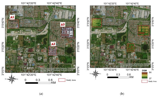
Figure 1. Wide-ranging whereabouts of study area: (a) aerial imageries for study areas A1, A2, and A3 and (b) digital surface model (DSM) for study areas A1, A2, and A3.

3.2. Data Used

Ground Data Solution Bhd captured LiDAR point cloud data and high-resolution aerial imageries across UPM and a portion of the Serdang area in 2015. The raw LiDAR information was acquired using the Riegel scanner on board the EC-120 helicopter, hovering at an average height above sea level of 600 m above the terrain surface. Using a focal length of 35 mm, a horizontal and vertical resolution of 72Dpi, and an exposure duration of 1/2500 s, the Canon EOS5D Mark III camera recorded the high-resolution aerial imagery (RGB color image) concurrently.

3.3. Methodology Applied

This study proposes a deep learning model to detect building objects from fused, very high-resolution aerial imagery and DSM derived from LiDAR. The general workflow of this model is in Figure 2.

Figure 2. General workflow of building extraction displaying various kernels of 2D-convolution when applying CNN-related techniques.

3.3.1. Overview of CNN

CNN’s are a sort of artificial neural network (ANN) used for image recognition and extraction. It is typically structured in a series of layers. The architecture allows the network to grasp several data representation levels, starting with low-level features in the lowest layers, such as corners and edges, and more acceptable feature information with high-level semantic information in the top layers. By utilizing a trainable 2-D convolutional filter, CNN takes advantage of the 2-D geometry of an input dataset (Equation (1)).

$$y_j^l=\sigma ({\displaystyle \sum }_{k\in -\frac{w}{2}\times \frac{w}{2}}{w}_{jk}\times y_k^{l-1}+b_j^l)$$

(1)

It connects single neurons at level l with a predefined limited area of fixed $W\times W$ from the beginning lay l − 1 and then gathers a weighted overall neuron accompanied by a specified activation function. The large one corresponds to a skew, with weights $jk$ shared through all neurons for each layer’s different dimensions. Compared to the typical multilayer perceptron (MLP), the allowed factors are significantly reduced in the model’s worth, which does not match since its class of neural networks lacks a weight distribution [34]. Furthermore, weight sharing brings translation equivariance, which is a form of a likened neural network attribute with $y_i=0=1$, and the bias can be assumed to go further than the weight. The activation function has the benefit of introducing nonlinearity into the network. After each convolutional layer CNN, the rectified linear unit (ReLU) is the highest available activation function. These aid in the conversion of all negative numbers to zero while positive values are maintained (Equation (2)).

$$y_{relu}^l=\max \left(0.y^l\right)$$

(2)

ReLU in neural networks can induce sparsity in the hidden units and are not affected by gradient vanishing issues [38].

CNN’s were initially designed for image classification issues, forecasting the suitable class linked with the input image. Henceforth, fully connected (FC) layers are the top layers of the network, enabling the combination of the complete image scene’s information. The last layer is a 1-D array, which comprises several neurons as likely classes, indicating class assignment as probabilities, frequently done via softmax normalization on distinct neurons. The classifier establishes the weights and biases that produce an optimal network classifier; it implies that the weight and biases will reduce the variance between the target and predicted values. Hence, misclassifications are dealt with by a loss function $L\left(x,t,p\right)$. Moreover, it is regularly applied across entropy loss functions (Equation (3)).

$$L\left(x,t,p\right)=-{\displaystyle \sum }_i{t}_{i}logp\left(x_i\right)$$

(3)

The mitigation against slowing down the learning rate (compared to the Euclidean distance loss function) gives an extra numerically unwavering gradient when paired with softmax normalization, where $x=\left\{x_1,\dots ,x_n\right\}$ is the set of input in the training dataset, and $t=\left\{t_1,\dots ,t_n\right\}$ is the equivalent set of target values. The $p\left(x_i\right)$ signifies the yield of the neural network for the input $x_i$. It curtails the logistic loss of the softmax outputs over the total patch. The gradient descent is a conventional approach to reduce the loss function. Furthermore, it is possible by its capacity to calculate the derivatives of the loss function with relation to parameter $\partial L\partial w_i$ and $\partial L\partial b_i$; updated using our learning rate $\lambda$ in the following way (Equations (4) and (5)):

$$w_i\leftarrow w_i-\frac{\partial L}{\partial w_i}$$

(4)

$$b_i\leftarrow b_i-\frac{\partial L}{\partial b_i}$$

(5)

The derivatives $\partial L$ and $\partial L$ $\partial w_i$ $\partial b_i$ are computed by the backpropagation algorithm typically applied in the stochastic gradient descent (SGD) optimization algorithm in insignificant batches for productivity.

This research aims to present a deep learning technique based on a CNN to categorize images and extract buildings from LiDAR images. Furthermore, the CNN model’s construction, training, and testing are used to classify images and extraction of building features. The CNN model’s performance, which is used to classify and extract building features, was evaluated using the confusion matrix concept. To this end, the language expresses a sense of balance between expressiveness and performance.

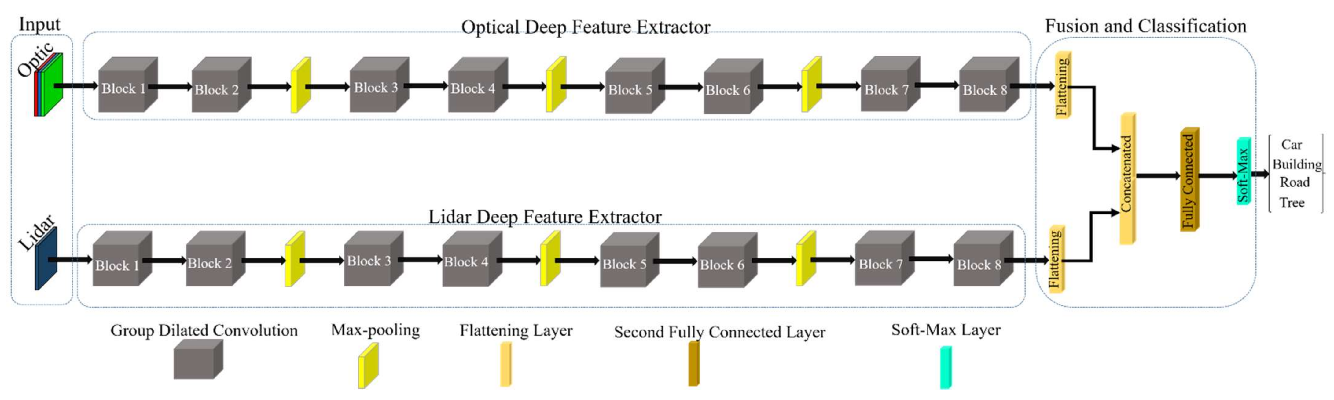
3.3.2. The Proposed Architecture of CNN

The structure of proposed deep learning based method has been inspired deep Siamese network [39]. Similarly, the proposed architecture for building extraction has double deep feature extraction streams to investigate the optical and DSM datasets and fusion them for building classification. The proposed architecture is applied in two main steps: (1) deep feature extraction by double streams channel and group convolution blocks and (2) classification. The deep features extraction has been conducted by 8 group convolution blocks in each stream. The three max-pooling layers are employed for reducing size feature map after convolution layers. The structure of both streams is similar while differing in the input. The first stream considers the deep feature extraction task for the optical dataset, and the second stream investigates the DSM dataset. Then, the extracted deep features from both streams are fused and are transformed into classification parts. The classification part has been carried out by a fully connected layer and a softmax layer. The fully connect layer is employed to represent as well the extracted the deep features by previous convolution layers. The softmax layer is employed to make a decision on input data.

Deep Feature Extraction

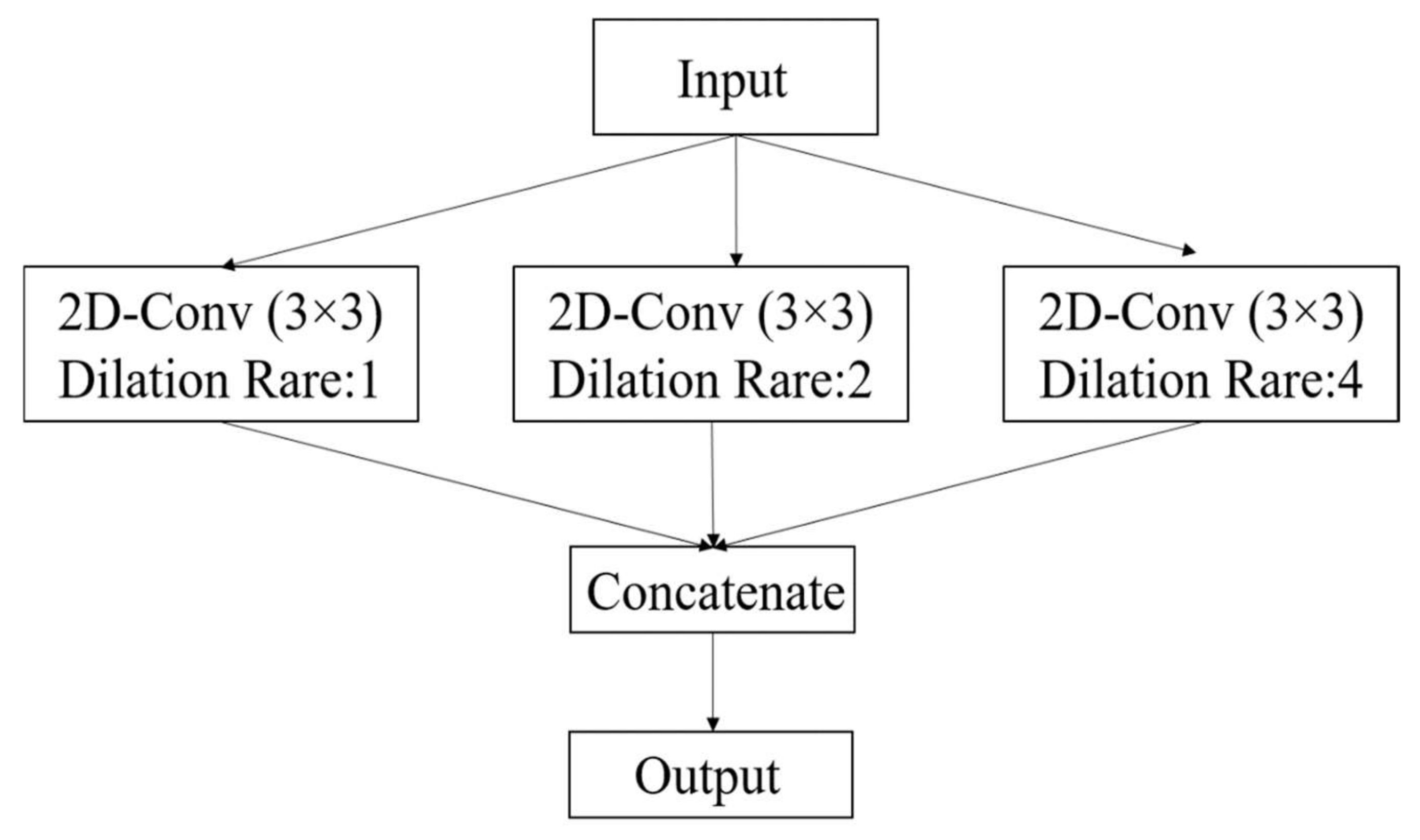
The deep learning-based methods are the most popular in the field of remote sensing due to their performance, providing promising results [40,41]. These deep learning-based methods able to represent the input data in an informative structure as well. The deep features are obtained by convolution layers in an automatic manner. The convolution layers extract the deep features by combining the spatial and spectral features from input data. Due to the different sizes of objects in the scene, many solutions have been proposed by studies (e.g., multi-scale convolution block or making it deeper) [42]. One suitable solution for variation of the scale of objects utilizes a dilated convolution block. The dilated convolution supports the exponential expansion of the receptive field without loss of resolution [39].

Figure 3 shows the structure of the proposed group convolution block in this study, in which we employed three dilated convolutions with different rates (1, 2, and 4). For a convolutional layer in the l_th layer, the computation is expressed according to Equation (6).

$$y^l=g\left(w^l{x}^{l-1}\right)+b^l$$

(6)

where x is the neuron input from the previous layer, $l-1$, $g$ is the activation function, $w$ is the weight template, and $b$ is the bias vector of current layer, $l$. The value ($v$) at position $\left(x,y\right)$ on the $j^{th}$ feature $i^{th}$ layer for the 3D-Dilated convolution layer is given by Equation (7).

$$v_{i,j}^{xy}=g(b_{i,j}+{\displaystyle \sum }_m{\displaystyle \sum }_{r=0}^{R_i-1}{\displaystyle \sum }_{s=0}^{S_i-1}{W}_{i,j,m}^{r,s,t}{v}_{i-1,m}^{\left(x+r\times d_1\right)\left(y+s\times d_2\right)})$$

(7)

where $b$ denotes bias, $g$ is the activation function, $m$ is the feature cube connected to the current feature cube in the ${\left(i-1\right)}^{th}$ layer, $W$ is the ${\left(r,s\right)}^{th}$ value of the kernel connected to the $m^{th}$ feature cube in the preceding layer, and $R$ and $S$ are the length, and width of the convolution kernel size, respectively. The $d_1$ and $d_2$ are also dilated convolution rates in length and width, respectively.

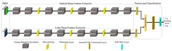
Figure 3. Proposed CNN model architecture.

Preprocessing

The proposed scheme involves four main sections: preprocessing our input data, data fusion, feature extraction and classification, and cleanup. The preprocessing stage includes but is not limited to the registration of ALS LiDAR. After filtering an intensity image, DSM were combined with RGB high-resolution aerial imagery. The generation of a DSM the raw point cloud was interpolated via the inverse weighted distance method algorithm of ArcGIS 10.7. After filtering, the point clouds were filtered to generate an intensity image, DEM, DSM, and nDSM combined with RGB from the high-resolution aerial imagery. At the same time, the DEM was generated from a non-ground point. Meanwhile, nDSM was derived based on the difference between DEM and DSM at 0.5 m spatial resolution.

Implementation Network

We integrate input data to train the CNN: a LiDAR dataset and high-resolution aerial imagery, DSM, and the high-resolution aerial imageries. We use three CNN templates to train them. Weights from other datasets, such as Alexnet, were not applied because the data was not RGB pre-trained; hence, the network was trained from scratch with random initialization.

Training and Testing Process

The dataset A2 was split randomly into two divisions: the first was used for the training process, which is 70% of the dataset, while the remaining 30% was used to test and validate the CNN model. Other two datasets, A1 and A3, were used to evaluate the transferability of the proposed framework. For the training process to be effective, the input parameters from the dataset, i.e., the CNN layers, and the training options must be defined. Training involves defining the optimizer, the number of iterations, and mini-batch size and defining the CNN layers. Therefore, after setting the above parameters, the training and testing process began. The model learned effective characteristics focusing on the increase in model accuracy and decreased model loss with time, categorizing the images and identifying building classes. The CNN model’s performance computation depended on the hyper-parameters: convolutional filters, dropout, and other layers. The CNN model was trained. Therefore, the model’s performance calculation effectively examines images, requiring more time for larger datasets. The CNN model was analyzed using the deep learning network analyzer application.

Quantitative Evaluation

The most popular indicator in classification is a confusion matrix. The horizontal axis is the expected label, and the vertical axis is the true label, as indicated in Table 1. The number that has been successfully classified is the diagonal element. Another criterion for classification is OA, which is used to assess the proportion of cases that are correctly classified [1]. As a result, the OA may be expressed as

$$OA=\frac{1}{N}{\displaystyle \sum }_{i=1}^n{C}_{ii}$$

(8)

where $i=1,2,\dots ,n$, and $C_{ii}$ is the number of correctly classified groups in i; $n$ is the number of classes, and $N$ is the overall sample size. To confirm reliability and measure classification precision, the kappa coeffcient was computed from the confusion matrix. As presented in Equations (9)–(11), it takes into account not only OA but also differences in the number of samples in each group.

$$k=\frac{p_o-p_e}{1-p_e}$$

(9)

$$p_o=\frac{1}{N}{\displaystyle \sum }_{i=1}^n{C}_{ii}$$

(10)

$$p_e=\frac{1}{N^2}{\displaystyle \sum }_{i=1}^n(C_{i+}\times C_{i+})$$

(11)

Table 1. The confusion matrix using the proposed method for Area1.

Classes	Non-Building	Building	Total	User Accuracy	Commission Error
(a) Area1 (DSM)
Non-Building	96.45%	18.24%	79.19%	94.92%	5.08%
Building	3.55%	81.76%	20.81%	86.70%	13.30%
Total	100.00%	100.00%	100.00%
Producer’s Accuracy	96.45%	81.76%		OA	Kappa Coefficient
Omission Error	3.55%	18.24%		93.20%	0.798
(b) Area1 (Optical)
Non-Building	92.80%	31.05%	79.17%	91.35%	8.65%
Building	7.20%	68.95%	20.83	73.06%	26.94%
Total	100%	100%	100%
Producer’s Accuracy	92.80%	68.95%		OA	Kappa Coefficient
Omission Error	7.20%	31.05%		87.53%	0.630
(c) Area1 (Fusion)
Non-Building	96.45%	18.24%	79.19%	94.92%	5.08%
Building	3.55%	81.76%	20.81%	86.70%	13.30%
Total	100%	100%	100%
Producer’s Accuracy	96.45%	81.76 %		OA	Kappa Coefficient
Omission Error	3.55%	18.24%		93.20%	0.787

The precision is a metric for determining the accuracy of each class, and it depicts the number classified into group $i$ by the model but that truly fit into the true class I ($i=1,2,\dots ,n$). It could be evaluated using the confusion matrix, and we can get the precision for each group for the $i-th$ classification as follows:

$$P_i=\frac{C_{ii}}{C+i}$$

(12)

4. Results and Discussion

4.1. Experimental Scenes and LiDAR Point Clouds

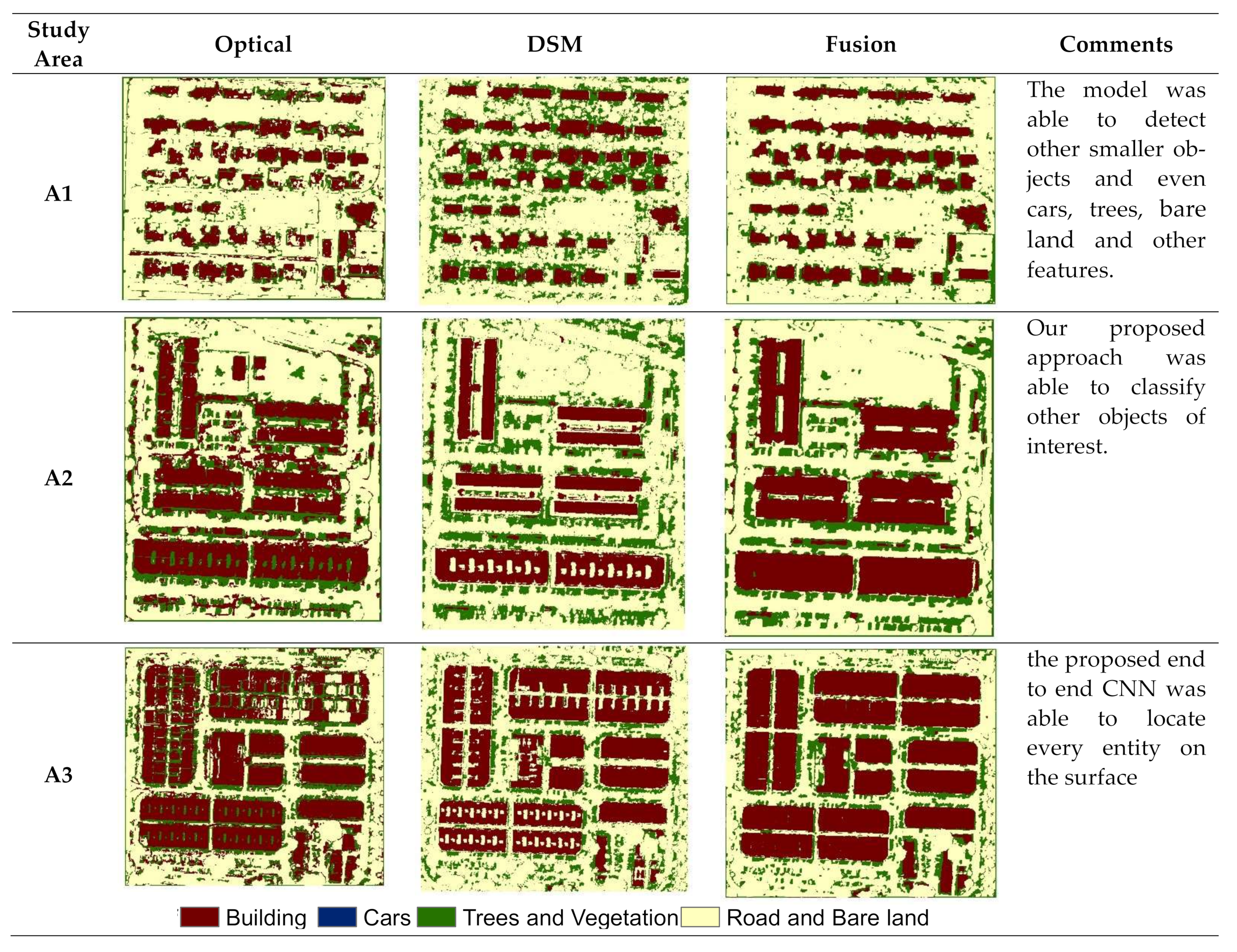
The building extraction studies reported in this article, involving the combination of LiDAR and very high-resolution area imagery data sources, were employed to know the performance of our proposed approach for binary building mask creation. The proposed building extraction model was evaluated on three datasets (i.e., Area1, Area2, and Area3) selected from (LiDAR and very high-resolution aerial imagery). The three different scenes are from subset areas. Area 1 is a fully residential neighborhood comprising detached small and medium houses with plenty of trees, while Area 2, on the other hand, consists of high-rise residential and business area buildings. In addition, Area 3 is a complex, dense urban development area with large building forms and roof patterns with fewer vegetation.

4.2. CNN Building Extraction Results

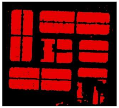
After training the network, three images of various subset areas (Area1, Area2, and Area3) were introduced as input for the network model to detect buildings from other features in the images. The pixels in the dataset are considered in two labels, explicitly building and non-building; since our interest was specifically on building objects, we took an interest in their classification and detection, as presented in Figure 4.

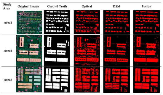
Figure 4. Classification outputs from three datasets. Optical, DSM, and fusion.

Table 1 shows the accuracy results in test area A1, where many small buildings and tall vegetation exist. We performed aerial assessment (percent) for each feature ground truth data, namely, the DSM, optical, and fusion to evaluate our model. From Table 1a, the OA was found to be 93.20%, while our kappa coefficient was found to be 0.798 for the DSM. For Table 1b, which is the optical, our OA was 87.53% with a kappa coefficient of 0.630, and lastly, for Table 1c, our OA was 93.20% and kappa was 0.787. Hence, we can conclude that the fusion of LiDAR and high-resolution aerial imagery and DSM only provided better performance than the optical alone.

Similarly, Table 2 presents test area A2, DSM (Table 2a) which has an OA of 91.06% and a kappa coefficient of 0.753, while optical (Table 2b) has an OA of 83.54% and kappa coefficient 0.606, and lastly, fusion (Table 2c) has an OA of 94.29% with a kappa coefficient of 0.859. We can deduce that fused output performed better than the DSM and optical.

Table 2. The confusion matrix using the proposed method for Area2.

Classes	Non-Building	Building	Total	User Accuracy	Commission Error
(a) Area2 (DSM)
Non-Building	97.76%	2.61%	79.25%	90.80%	9.20%
Building	2.24%	72.39%	20.75%	92.06%	7.94%
Total	100%	100%	100%
Producer’s Accuracy	97.76%	72.39%		OA	Kappa Coefficient
Omission Error	2.24%	27.61%		91.06%	0.753
(b) Area2 (Optical)
Non-Building	84.56%	19.29%	67.33%	92.44%	7.56%
Building	15.44%	80.71%	32.67%	65.20%	34.80%
Total	100%	100%	100%
Producer’s Accuracy	84.56%	80.71%		OA	Kappa Coefficient
Omission Error	15.44%	19.29%		83.5407%	0.606
(c) Area2 (Fusion)
Non-Building	93.72%	4.10%	70.07%	98.46%	1.54%
Building	6.28%	95.90%	29.93%	84.56%	15.44%
Total	100%	100%	100%
Producer’s Accuracy	93.72%	95.90%		OA	Kappa Coefficient
Omission Error	6.28%	4.10%		94.29%	0.859

Table 1 shows the accuracy results in test area A3. From Table 3a (DSM), we can deduce that the OA was 87.91%. In comparison, the kappa coefficient was 0.748, and optical (Table 3b) was 80.85% for OA. The kappa coefficient was 0.608, and in addition, in Table 3c (Fusion), the value was 91.87% for OA while the kappa was 0.834. This is an indication that our combination of LiDAR and high-resolution imagery is better for feature extraction than using only the DSM alone or the optical only.

Table 3. The confusion matrix using the proposed method for Area3.

Classes	Non-Building	Building	Total	User Accuracy	Commission Error
(a) Area3 (DSM)
Non-Building	85.30%	7.43%	57.24%	95.32%	4.68%
Building	14.70%	92.57%	42.76%	78.00%	22.00%
Total	100%	100%	100%
Producer’s Accuracy	85.30%	92.57%		OA	Kappa Coefficient
Omission Error	14.70%	7.43%		87.91%	0.748
(b) Area3 (Optical)
Non-Building	83.73%	23.00%	57.77%	82.97%	17.03%
Building	16.27%	77.00%	42.23%	77.95%	22.05%
Total	100%	100%	100%
Producer’s Accuracy	83.73%	77.00%		OA	Kappa Coefficient
Omission Error	16.27%	23.00%		80.85%	0.608
(c) Area3 (Fusion)
Non-Building	92.51%	8.98%	56.79%	93.24%	6.76%
Building	7.49%	91.02%	43.21%	90.07%	9.93%
Total	100%	100%	100%
Producer’s Accuracy	92.51%	91.02%		OA	Kappa Coefficient
Omission Error	7.49%	8.98%		91.8715%	0.834

The overall accuracies of the three study areas are: A1, 93.21% for DSM, 87.54% for optical image, and 93.21% for the fusion. Kappa coefficients of 0.798, 0.630, and 0.798, respectively, for study area A1. Moreover, for A2, the DSM was 91.07%, optical was 87.54%, and 93.21% for the fusion with kappa coefficients of 0.798, 0.630, and 0.798 respectively. In addition, for station A3, the value is 87.92% for DSM, 80.85% for optical, and 91.87% for the fusion. In totality, the fusion of the DSM and optical image provides the highest accuracy in detecting and extracting small buildings in location A1. The evaluation is summarized in Table 4. here, the OA and the kappa coefficient were used, and a comparison between their various performances is presented. The optical image generated output underperformed with the lowest accuracy compared to other parameters in all the study areas.

Table 4. The summary of the evaluation of the method using the OA and Kappa coefficient.

Datasets/Study Area	A1		A2		A3
	OA	Kappa	OA	Kappa	OA	Kappa
DSM	93.21%	0.798	91.07%	0.753	87.92%	0.748
Optical	87.54%	0.630	83.54%	0.606	80.85%	0.608
Fusion	93.21%	0.798	94.30%	0.859	91.87%	0.834

The results are better by fusion in area A2, which happens to be a highly complex area with a value of 94.30% and a kappa coefficient of 0.859, which is better than the optical image or DSM alone. Area A1 precedes this with a value of 93.21% with a kappa coefficient of 0.798, which shows a slight equivalent output with the DSM. This implies that at subset A1, there was not much difference in the results between the DSM and the fused output due to the nature of the buildings found, some of which are occluded and equally detached or of moderate height. The same scenario occurs in areas with mixed building forms, e.g., A3, where the OA is 91.87% and kappa coefficient is 0.834, although the fusion took the lead in the detection and classification.

The summary of results in the test areas A1, A2, and A3 in Figure 5 relates the different classification (building, cars, trees and vegetations, and road and bare land) and detection results from the proposed model. It can be seen that the image of the optical was used to detect buildings of various forms. However, the accuracy was just low compared to the DSM. The output from the DSM provided us with relatively higher accuracy compared to the optical. However, as demonstrated in Figure 5, the optical image fails to capture the voids between buildings and the geometry of the buildings in densely built-up areas. Note that by using the DSM to detect and classify objects, the accuracy was better. Hence, to further improve our result, we fused the LiDAR DSM and high-resolution aerial imagery to produce our fused image. The performance of this was very profound, and it was able to detect complex building objects found within the test area.

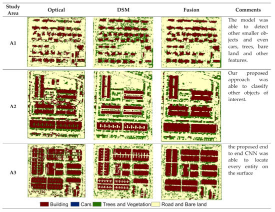
Figure 5. Classification outputs of building extraction displaying other detected features from end-to-end CNN approach.

In addition, a morphological dilation filter was used to correct the extracted buildings, compensating for the effects of shadow on building boundaries. The accuracy of the building per area is shown in Table 5. The difference between the accuracies of A1 and A3 in terms of their variation stood at 93.09% with a kappa coefficient = 0.788 for A1 in contrast to 92.16% with a kappa coefficient = 0.840 for A3. From this evaluation, we can infer that morphological operation does not always produce a refined result. Although it worked for A1, it did not work for A3. Moreover, the algorithm was able to detect and classify other features; however, because our focus is major on building features, the other features were eliminated. The end-to-end algorithm stood a chance of being used in the classification of other features and not just sand, ground, bare ground, and even mobile cars.

Table 5. The result of applying morphology to the proposed CNN technique.

Study Area	Fusion	Result Using Morphology	Discussion
A1		OA = 93.09% Kappa Coefficient = 0.78	A morphological dilation filter was used to correct the extracted buildings, compensating for the effects of shadow on building boundaries. Before applying morphological operation at area A1, the OA and the kappa coefficient were 93.22% and 0.798, respectively. After applying the OA, and kappa coefficient rose to 93.09% and 0.788. It implies the operation is effective for area A1.
A3		OA = 92.16% Kappa Coefficient = 0.840	The same operation was performed on area A3. The OA and kappa coefficient value was 92.16%, 0.840, and after this operation on A3, the new OA and kappa coefficient became 91.87%, 0.834. at the same time, the performance was poor for A3. Hence morphological operation cannot provide total refinement of all forms of building objects.

5. Conclusions

CNN’s have achieved remarkable solutions for various fields, including geospatial studies, and there is growing interest in LiDAR. However, deep learning has been the preferred method for a range of challenging tasks, including image classification and object detection and modelling. In this study, the end-to-end framework founded on deep learning is proposed for urban building detection and classification. A multi-dimensional convolution layer structure is used in the proposed scheme. Moreover, the proposed approach uses the advantages of fusion of LiDAR and high-resolution aerial imagery spectral RGB and deep feature differencing. We evaluated the result for urban buildings extraction for three different building forms and structures in difficult metropolitan locations of Serdang, in Selangor State, Malaysia. The results reveal that relying solely on high-resolution aerial imagery classification leads to low classification accuracy.

On the other hand, the application of DSM tends to increase the detection rate because it can correctly distinguish between buildings and ground characteristics. Low-level structures such as tree branches may be difficult to spot. This challenging issue can be solved by employing LiDAR and DSM integration, which uses spectral and height features to achieve high accuracy for small building categorization. There were some noticeable irregularities in some sections in the resulting building mask, due to occlusion, shadow by vegetation, or taller buildings, which makes building extracting in urban areas difficult. Lastly, our approach is fast, reliable, and productive for mapping buildings in the urban area for proper planning and mitigation against hazards, wildfires, and other related issues. The fusion of LiDAR with other ancillary datasets provides a rapid solution to urban remote sensing problems. This work demonstrated CNN’s capacity to effectively categorize building features using very-high-resolution aerial imageries and the LiDAR dataset, compared to adopting a single source of imageries, and indicated that dataset fusion is plausible. There is a need to evaluate the sensitivity of deep learning methods on mega multifaceted building structures such as the stadiums and high-rise buildings which will be the subject of future research work.

References

- Al-Najjar, H.A.H.; Kalantar, B.; Pradhan, B.; Saeidi, V. Land Cover Classification from fused DSM and UAV Images Using Convolutional Neural Networks. Remote Sens. 2019, 11, 1461. [Google Scholar] [CrossRef] [Green Version]
- Pradhan, B.; Al-Najjar, H.A.H.; Sameen, M.I.; Tsang, I.; Alamri, A.M. Unseen land cover classification fromhigh-resolution orthophotos using integration of zero-shot learning and convolutional neural networks. Remote Sens. 2020, 12, 1676. [Google Scholar] [CrossRef]
- Kalantar, B.; Ueda, N.; Al-Najjar, H.A.H.; Halin, A.A. Assessment of convolutional neural network architectures for earthquake-induced building damage detection based on pre-and post-event orthophoto images. Remote Sens. 2020, 12, 3529. [Google Scholar] [CrossRef]
- Dong, Y.; Zhang, L.; Cui, X.; Ai, H.; Xu, B. Extraction of buildings from multiple-view aerial images using a feature-level-fusion strategy. Remote Sens. 2018, 10, 1947. [Google Scholar] [CrossRef] [Green Version]
- Rottensteiner, F.; Sohn, G.; Gerke, M.; Wegner, J.D.; Breitkopf, U.; Jung, J. Results of the ISPRS benchmark on urban object detection and 3D building reconstruction. ISPRS J. Photogramm. Remote Sens. 2014, 93, 256–271. [Google Scholar] [CrossRef]
- Alidoost, F.; Arefi, H. A CNN-Based Approach for Automatic Building Detection and Recognition of Roof Types Using a Single Aerial Image. PFG J. Photogramm. Remote Sens. Geoinf. Sci. 2018, 86, 235–248. [Google Scholar] [CrossRef]
- Gibril, M.B.A.; Kalantar, B.; Al-Ruzouq, R.; Ueda, N.; Saeidi, V.; Shanableh, A.; Mansor, S.; Shafri, H.Z.M. Mapping heterogeneous urban landscapes from the fusion of digital surface model and unmanned aerial vehicle-based images using adaptive multiscale image segmentation and classification. Remote Sens. 2020, 12, 1081. [Google Scholar] [CrossRef] [Green Version]
- Grigillo, D.; Kanjir, U. Urban Object Extraction from Digital Surface Model and Digital Aerial Images. ISPRS Ann. Photogramm. Remote Sens. Spat. Inf. Sci. 2012, 3, 215–220. [Google Scholar] [CrossRef] [Green Version]
- Tomljenovic, I.; Höfle, B.; Tiede, D.; Blaschke, T. Building extraction from Airborne Laser Scanning data: An analysis of the state of the art. Remote Sens. 2015, 7, 3826–3862. [Google Scholar] [CrossRef] [Green Version]
- Fritsch, D.; Klein, M.; Gressin, A.; Mallet, C.; Demantké, J.Ô.; David, N.; Heo, J.; Jeong, S.; Park, H.H.K.; Jung, J.; et al. Generating 3D city models without elevation data. ISPRS J. Photogramm. Remote Sens. 2017, 64, 1–18. [Google Scholar] [CrossRef] [Green Version]
- Yang, H.; Wu, P.; Yao, X.; Wu, Y.; Wang, B.; Xu, Y. Building extraction in very high resolution imagery by dense-attention networks. Remote Sens. 2018, 10, 1768. [Google Scholar] [CrossRef] [Green Version]
- Fernandes, D.; Silva, A.; Névoa, R.; Simões, C.; Gonzalez, D.; Guevara, M.; Novais, P.; Monteiro, J.; Melo-Pinto, P. Point-cloud based 3D object detection and classification methods for self-driving applications: A survey and taxonomy. Inf. Fusion 2021, 68, 161–191. [Google Scholar] [CrossRef]
- Zhou, Z.; Gong, J. Automated residential building detection from airborne LiDAR data with deep neural networks. Adv. Eng. Inform. 2018, 36, 229–241. [Google Scholar] [CrossRef]
- Park, Y.; Guldmann, J.-M.M. Creating 3D city models with building footprints and LIDAR point cloud classification: A machine learning approach. Comput. Environ. Urban Syst. 2019, 75, 76–89. [Google Scholar] [CrossRef]
- Chang, Z.; Yu, H.; Zhang, Y.; Wang, K. Fusion of hyperspectral CASI and airborne LiDAR data for ground object classification through residual network. Sensors 2020, 20, 3961. [Google Scholar] [CrossRef] [PubMed]
- Elsayed, H.; Zahran, M.; Elshehaby, A.R.; Salah, M.; Elshehaby, A. Integrating Modern Classifiers for Improved Building Extraction from Aerial Imagery and LiDAR Data. Am. J. Geogr. Inf. Syst. 2019, 2019, 213–220. [Google Scholar] [CrossRef]
- Xie, Y.; Zhu, J.; Cao, Y.; Feng, D.; Hu, M.; Li, W.; Zhang, Y.; Fu, L. Refined Extraction of Building Outlines from High-Resolution Remote Sensing Imagery Based on a Multifeature Convolutional Neural Network and Morphological Filtering. IEEE J. Sel. Top. Appl. Earth Obs. Remote Sens. 2020, 13, 1842–1855. [Google Scholar] [CrossRef]
- Awrangjeb, M.; Ravanbakhsh, M.; Clive, S.F. Automatic detection of residential buildings using LIDAR data and multispectral imagery. ISPRS Jounal Photogramm. Remote Sens. 2013, 53, 1689–1699. [Google Scholar] [CrossRef] [Green Version]
- Gilani, S.A.N.; Awrangjeb, M.; Lu, G. Fusion of LiDAR data and multispectral imagery for effective building detection based on graph and connected component analysis. Int. Arch. Photogramm. Remote Sens. Spat. Inf. Sci. 2015, 40, 65–72. [Google Scholar] [CrossRef] [Green Version]
- Maltezos, E.; Doulamis, A.; Doulamis, N.; Ioannidis, C. Building extraction from LiDAR data applying deep convolutional neural networks. IEEE Geosci. Remote Sens. Lett. 2019, 16, 155–159. [Google Scholar] [CrossRef]
- Chen, C.; Gong, W.; Hu, Y.; Chen, Y.; Ding, Y.; Vi, C.; Vi, W.G. Learning Oriented Region-based Convolutional Neural Networks for Building Detection in Satellite Remote Sensing Images. Int. Arch. Photogramm. Remote Sens. Spat. Inf. Sci. 2017, XLII, 6–9. [Google Scholar] [CrossRef] [Green Version]
- Wierzbicki, D.; Matuk, O.; Bielecka, E. Polish cadastre modernization with remotely extracted buildings from high-resolution aerial orthoimagery and airborne LiDAR. Remote Sens. 2021, 13, 611. [Google Scholar] [CrossRef]
- Lu, T.; Ming, D.; Lin, X.; Hong, Z.; Bai, X.; Fang, J. Detecting building edges from high spatial resolution remote sensing imagery using richer convolution features network. Remote Sens. 2018, 10, 1496. [Google Scholar] [CrossRef] [Green Version]
- Li, W.; Liu, H.; Wang, Y.; Li, Z.; Jia, Y.; Gui, G. Deep Learning-Based Classification Methods for Remote Sensing Images in Urban Built-Up Areas. IEEE Access 2019, 7, 36274–36284. [Google Scholar] [CrossRef]
- Lai, X.; Yang, J.; Li, Y.; Wang, M. A building extraction approach based on the fusion of LiDAR point cloud and elevation map texture features. Remote Sens. 2019, 11, 1636. [Google Scholar] [CrossRef] [Green Version]
- Wen, C.; Yang, L.; Li, X.; Peng, L.; Chi, T. Directionally constrained fully convolutional neural network for airborne LiDAR point cloud classification. ISPRS J. Photogramm. Remote Sens. 2020, 162, 50–62. [Google Scholar] [CrossRef] [Green Version]
- Al-Najjar, H.A.H.; Pradhan, B.; Sarkar, R.; Beydoun, G.; Alamri, A. A New Integrated Approach for Landslide Data Balancing and Spatial Prediction Based on Generative Adversarial. Remote Sens. 2021, 13, 4011. [Google Scholar] [CrossRef]
- Al-Najjar, H.A.H.; Pradhan, B. Spatial landslide susceptibility assessment using machine learning techniques assisted by additional data created with generative adversarial networks. Geosci. Front. 2021, 12, 625–637. [Google Scholar] [CrossRef]
- Mousa, Y.A.; Helmholz, P.; Belton, D.; Bulatov, D. Building detection and regularisation using DSM and imagery information. Photogramm. Rec. 2019, 34, 85–107. [Google Scholar] [CrossRef] [Green Version]
- Sherrah, J. Fully Convolutional Networks for Dense Semantic Labelling of High-Resolution Aerial Imagery. arXiv 2016, arXiv:Abs/1606.02585. [Google Scholar]
- Wen, Q.; Jiang, K.; Wang, W.; Liu, Q.; Guo, Q.; Li, L.; Wang, P. Automatic building extraction from google earth images under complex backgrounds based on deep instance segmentation network. Sensors 2019, 19, 333. [Google Scholar] [CrossRef] [PubMed] [Green Version]
- Ghamisi, P.; Li, H.; Soergel, U.; Zhu, X.X. Hyperspectral and LiDAR fusion using deep three-stream convolutional neural networks. Remote Sens. 2018, 10, 1649. [Google Scholar] [CrossRef] [Green Version]
- Xie, L.; Zhu, Q.; Hu, H.; Wu, B.; Li, Y.; Zhang, Y.; Zhong, R. Hierarchical regularization of building boundaries in noisy aerial laser scanning and photogrammetric point clouds. Remote Sens. 2018, 10, 1996. [Google Scholar] [CrossRef] [Green Version]
- Bittner, K.; Adam, F.; Cui, S.; Körner, M.; Reinartz, P. Building Footprint Extraction From VHR Remote Sensing Images Combined With Normalized DSMs Using Fused Fully Convolutional Networks. IEEE J. Sel. Top. Appl. Earth Obs. Remote Sens. 2018, 11, 2615–2629. [Google Scholar] [CrossRef] [Green Version]
- Gilani, S.A.N.; Awrangjeb, M.; Lu, G. An Automatic Building Extraction and Regularisation Technique Using LiDAR Point Cloud Data and Orthoimage. Remote Sens. 2016, 8, 258. [Google Scholar] [CrossRef] [Green Version]
- Nahhas, F.H.; Shafri, H.Z.M.; Sameen, M.I.; Pradhan, B.; Mansor, S. Deep Learning Approach for Building Detection Using LiDAR-Orthophoto Fusion. J. Sens. 2018, 2018, 1–12. [Google Scholar] [CrossRef] [Green Version]
- Li, D.; Shen, X.; Yu, Y.; Guan, H.; Li, J.; Zhang, G.; Li, D. Building extraction from airborne multi-spectral LiDAR point clouds based on graph geometric moments convolutional neural networks. Remote Sens. 2020, 12, 3186. [Google Scholar] [CrossRef]
- Zhang, L.; Li, Z.; Li, A.; Liu, F. Large-scale urban point cloud labeling and reconstruction. ISPRS J. Photogramm. Remote. Sens. 2018, 138, 86–100. [Google Scholar] [CrossRef]
- Seydi, S.T.; Hasanlou, M.; Amani, M. A new end-to-end multi-dimensional CNN framework for land cover/land use change detection in multi-source remote sensing datasets. Remote Sens. 2020, 12, 2010. [Google Scholar] [CrossRef]
- Seydi, S.T.; Rastiveis, H. A Deep Learning Framework for Roads Network Damage Assessment Using Post-Earthquake Lidar Data. Int. Arch. Photogramm. Remote Sens. Spat. Inf. Sci. 2019, XLII, 12–14. [Google Scholar] [CrossRef] [Green Version]
- Seydi, S.T.; Hasanlou, M. A New Structure for Binary and Multiple Hyperspectral Change Detection Based on Spectral Unmixing and Convolutional Neural Network. Measurement 2021, 186, 110137. [Google Scholar] [CrossRef]
- Seydi, S.T.; Hasanlou, M.; Amani, M.; Huang, W. Oil Spill Detection Based on Multiscale Multidimensional Residual CNN for Optical Remote Sensing Imagery. IEEE J. Sel. Top. Appl. Earth Obs. Remote Sens. 2021, 14, 10941–10952. [Google Scholar] [CrossRef]
Publisher’s Note: MDPI stays neutral with regard to jurisdictional claims in published maps and institutional affiliations. |
© 2021 by the authors. Licensee MDPI, Basel, Switzerland. This article is an open access article distributed under the terms and conditions of the Creative Commons Attribution (CC BY) license (https://creativecommons.org/licenses/by/4.0/).