Abstract
Urban building morphology has a significant impact on the urban thermal environment (UTE). The sky view factor (SVF) is an important structure index of buildings and combines height and density attributes. These factors have impact on the land surface temperature (LST). Thus, it is crucial to analyze the relationship between SVF and LST in different spatial-temporal scales. Therefore, we tried to use a building vector database to calculate the SVF, and we used remote sensing thermal infrared band to retrieve LST. Then, we analyzed the influence between SVF and LST in different spatial and temporal scales, and we analyzed the seasonal variation, day–night variation, and the impact of building height and density of the SVF–LST relationship. We selected the core built-up area of Beijing as the study area and analyzed the SVF–LST relationship in four periods in 2018. The temporal experimental results indicated that LST is higher in the obscured areas than in the open areas at nighttime. In winter, the maximum mean LST is in the open areas. The spatial experimental results indicate that the SVF and LST relationship is different in the low SVF region, with 30 m and 90 m pixel scale in the daytime. This may be the shadow cooling effect around the buildings. In addition, we discussed the effects of building height and shading on the SVF–LST relationship, and the experimental results show that the average shading ratio is the largest at 0.38 in the mid-rise building area in winter.
1. Introduction
Rapid urbanization has resulted in increased urban population density, urban expansion, and the conversion of a large number of natural surfaces to artificial surfaces and buildings. The increases of impervious surfaces and building walls and the decrease of vegetation cover affect the urban thermal environment [1,2]. Residents that have lived in urban centers for a long time feel the increased effects of the surface urban heat island, which makes people feel physically and psychologically uncomfortable and affects the comfort level and quality of life of an urban living environment [3,4]. Therefore, the study of its influencing factors and mechanisms is particularly important in order to propose a scientific and reasonable strategy to alleviate the urban thermal environment [5,6].
Urban building morphology is an important influencing factor of an urban thermal environment. Most research exploring the influence of building morphology on an urban thermal environment used the two-dimensional and three-dimensional characteristics of buildings [7,8,9].
The horizontal characteristics of the buildings change the type of the original land cover. This affects the process of solar radiation absorption and the emission of long-wave radiation from the ground [10]. Relevant scholars characterized the building characteristics by building density. The land surface temperature describes the urban thermal environment, using the correlation analysis of the building density and LST, and the scholars found that the relationship between LST and building density is moderately correlated [11]. Li used Landsat imagery data to extract impermeable surface cover (ISP) and land surface temperature in Beijing and quantitatively analyzed the spatial distribution characteristics of both [12]. However, it was not comprehensive to consider only the relationship between the two-dimensional characteristics of buildings and the urban thermal environment [13].
Conversely, the different heights of the buildings’ canopy morphology change the radiation transmission process between the sun and the surface, which includes the absorption of solar radiation and the emission of long-wave radiation from the surface [14,15]. Therefore, scholars focused on the study of the influence of three-dimensional building morphology on the urban thermal environment [16,17,18]. By analyzing the relationship between the spatial distribution of surface temperature and urban morphology, related scholars have shown that the sky view factor has a higher relevance of influence on LST than building density [19]. Quantitative indicators of the three-dimensional form of the building include building height (BH) [20,21], sky view factor (SVF) [22,23], building floor area ratio (FAR) [24], building volume (BV) [25], etc. Where SVF is a dimensionless value ranging from 0 to 1, 0 indicates a completely obscured area, and 1 indicates an open area. From a radiation perspective, SVF is defined as the ratio of radiation received (or emitted) from the sky by a plane to the radiation emitted (or received) by the entire unit hemisphere radiation environment [26]. From a geometric point of view, SVF is the proportion of the visible area of the sky per unit range within an urban street due to shading by buildings or trees [27].
Since SVF links the dual definition of building morphology and solar radiation, an increasing amount of studies are focusing on the SVF–LST relationship. Zhang [28] used the data from meteorological stations to calculate the temperature parameters, while the SVF is calculated by a geometric method using the 3D database of buildings. The relationship between SVF and LST was negatively correlated at night and positively correlated at daytime, and there are differences between the two relationships at different spatial scales. However, because the weather station data are point data with few statistical values, the fitted relationship between continuous SVF and LST cannot be obtained. In addition, Scarano [29] obtained the statistical results of the relationship between continuous SVF and LST using Landsat8 thermal infrared image data to invert the surface temperature by radiative transfer equation, and the results showed that the two were positively correlated during the daytime. Scarano [30] inverted the LST from satellite images and the UAV data and analyzed the SVF–LST relationship at different spatial resolutions, concluding that the choice of the optimal study image scale was related to the image scale of the smallest feature of interest in the study area. However, the SVF–LST relationship is missing for the analysis of regions with different feature characteristics at local scales.
By summarizing the existing studies, the problems of current studies on the influence of SVF on urban land surface temperature are: (1) uncertainties in the SVF–LST relationship exist at different research image scales; (2) differences in the SVF–LST relationship of different season and diurnal.
To address the aforementioned problems, this study obtains continuous LST results from Landsat-8 thermal infrared images and ASTER_003 data. The continuous SVF results of the study area are further extracted by a geometric method based on the building vector data. Since SVF is a parameter that can describe the three-dimensional morphology of urban buildings, and previous studies have shown that SVF is closely related to an urban microclimate. This paper takes SVF as the main factor to explore the relationship between SVF and spatial and temporal distribution of land surface temperature. In addition, the cooling effect of building shadows is considered, and three types of different building height areas are used as test areas to further analyze the effect on the SVF–LST relationship.
2. Materials and Methods
2.1. Study Area and Data
Beijing is the capital of China and is located between 115°42′–117°24′E and 39°32′–41°36′N. The location of the study area is shown in Figure 1a. With warm temperate semi-humid semi-arid monsoon climate, the intra-annual temperature ranges between −17.0–41.9 °C (http://bj.cma.gov.cn/, accessed on 16 June 2021). In Beijing, summer is hot and rainy, while winter is cold and dry. As a modern city in China, Beijing is known to have a high level of urbanization and is the political, economic and cultural center.
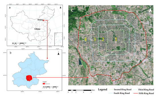
Figure 1.
Location of the study area. (a) Location of Beijing in China; (b) study area in Beijing; (c) four study areas divided by the ring road.
We selected the built-up area of Beijing as the study area, located within the fifth ring road. Area 1 is the second ring road region, area 2 is the region between the third ring road and the second ring road, area 3 is the region between the fourth ring road and third ring road, and area 4 is the region between the fifth ring road and fourth ring road, as shown in Figure 1c, where it is well built with a dense and heterogeneous layout of urban buildings. In addition, building form is one of the important factors affecting LST. Therefore, the built-up area of Beijing, with high urbanization and seasonal variation of climate, are conducive to the study of the influence of changes in sky view factors, caused by buildings, on urban LST.
Remote sensing images of Beijing and building data were used in this study. To analyze the daytime and seasonal differences between SVF and LST, four views of thermal infrared imagery from Landsat-8 with spatial resolution of 100 m, on 3 February 2018, 27 June 2018, 1 October 2018 and 4 December 2018 were used (https://earthexplorer.usgs.gov/, accessed on 15 May 2021). To analyze daytime and nighttime differences between SVF and LST, two views of ASTER_v8_003 surface temperature products were selected, which are daytime data with 11.17 a.m. on 5 October 2020 and 22:17 p.m. In addition, nighttime data on 23 September 2018 with spatial resolution of 90 m was analyzed (https://search.earthdata.nasa.gov/, accessed on 10 June 2021). The remote sensing images are shown in Table 1.

Table 1.
Satellite images data information.
The building data were in vector format and included the number of building floor and footprints of all the buildings in the built-up area in Beijing and were derived from the resource and environment science and data center (https://www.resdc.cn, accessed on 15 May 2021). The SVF was extracted using building floor and building bottom 2018 Beijing building vector data, where the height of each floor of the building was assumed to be 3 m for obtaining the urban building height.
2.2. Methods
2.2.1. Retrieval of the LST
The radiative transfer equation (RTE) was used to calculate the LST of the study area, and the thermal infrared band that is band ten of Landsat-8 was the input. This method was used to retrieve the LST on 3 February 2018, 27 June 2018, 1 October 2018 and 4 December 2018. In this paper, the main retrieval methods included radiometric calibration, blackbody radiation calculation, and LST retrieval [31]. The equation for the thermal infrared radiometric brightness is:
where represents the wavelength (); and are the scale factor obtained from the Landsat-8 satellite header file; DN represents the remote sensing image element value. The thermal infrared radiometric brightness is obtained by radiometric calibration of the above parameter.
where (LST) is the blackbody emissivity at a temperature of LST; is the thermal infrared radiance () obtained by radiometric calibration; , and is the thermal infrared band upward radiance, downward radiance and atmospheric transmittance obtained from the NASA website (http://atmcorr.gsfc.nasa.gov/, accessed on 15 May 2021) respectively; is the surface emissivity. Among them, the surface emissivity was estimated by the normalized vegetation index (NDVI) threshold method, which first calculates the vegetation coverage of each scene image by NDVI, calculates the temperature ratios of vegetation, bare soil and buildings in the surface, and then calculates the emissivity of different feature types by using the vegetation coverage and temperature ratios.
where and for Landsat-8.
2.2.2. Building SVF Calculation
The 3D forms of urban buildings are complex and vary depending on their height and structure. Previous studies used the aspect ratio as an indicator of the 3D morphology of buildings [27]. However, the width between buildings is more time-consuming and laborious to obtain in a larger study area. Furthermore, the previous definition of the SVF is the ratio of the amount of radiation received (or emitted) from the surface of the earth to the amount of radiation emitted (or received) from the entire hemisphere. The SVF can be explained from both solar radiation and building geometry perspectives. In addition, the SVF of the 3D building dataset can be quickly extracted by a computer program [32]. The method was programmed using the Relief Visualization Toolbox (RVT) based on IDL environment in the Environment for Visualizing Images (ENVI) [33]. The principle of spatial three-dimensional angle geometry is shown in Figure 2. The equation for calculating the SVF using the stereo angle principle is:
where R denotes the maximum radius of the observation range of a calculated point, indicates the maximum value of the building height within the observation range, indicates the number of search azimuths, is the azimuth angle within the observation range, and β indicates the maximum height angle obtained from the building height in the search for the maximum radius and azimuth angle. SVF indicates the percentage of the portion of the sky that can be seen at an observation point location.
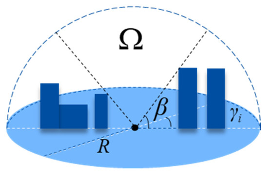
Figure 2.
Hemispheric model for the sky view factor calculation using RVT.
2.2.3. Statistical Analyses of the SVF and LST
This paper presents a quantitative analysis of the effect of SVF on the spatial distribution of LST. The statistical results of the relationship between the 3D morphology of buildings and the urban surface temperature distribution are analyzed by correlation analysis.
In this paper, the fitted regression equations are analyzed using the Pearson correlation coefficient. This measure can illustrate the relationship between two continuous variables. The calculation equation is:
where n is the total number of samples in a set, is the sample data value, and is the sample mean.
The first step is to process the results of the building parameters and the LST parameters. The average of the response parameters is taken at 0.01 intervals according to the SVF. Then, the average values of the parameters are plotted on a scatter plot. The correlation of the parameters is then described using linear and nonlinear fitting methods. Finally, the confidence level of the fit is tested by the mean squared error and significance level. Besides, the running time of each step of the experiment includes the retrieval of the LST, the calculation of building SVF, and the statistical analyses of the SVF and LST, as shown in Table A1.
3. Results and Discussion
3.1. The Building Characteristics at Different Areas
The building floor attributes of the building vector data were rasterized, the raster data were resampled to 30 m resolution, and the continuous SVF results extracted by RVT are shown in Figure 3a. It can be seen that the overall SVF distribution within the fifth Ring Road area of Beijing is higher in the lower and denser building height areas, such as the second Ring Road area and the edge of the fifth Ring Road and is lower in the higher and sparser building height areas, such as the third Ring Road and the area around the third Ring Road.
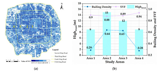
Figure 3.
Study area characteristics: (a) calculated SVF results of the study area; (b) buildings.
The average height and building density of the buildings describe the characteristics between different study areas. The building density of each study area is calculated using the building footprint attributes, and the results are shown in Figure 3b. It shows that the building density is lower in area 1 and area 4, while the building density is higher in area 2 and area 3. The building heights are approximately the same, with the heights in area 1 and area 4 being lower than in area 2 and area 3. In addition, the differences in the average SVF values in the four study areas are small, but it shows that the SVF values are larger in the regions with lower and less dense buildings and vice versa.
3.2. Seasonal Variation of SVF–LST Relationship
The results of the retrieval of land surface temperature in the study area from Landsat-8 remote sensing images selected for the fourth period of 2018 are shown in Figure 4a–d. The retrieval results are divided into five levels according to the natural break method [34], and the retrieval results show that the spatial distribution of land surface temperature varies greatly in different seasons. From the retrieval results of land surface temperature on 3 February 2018, the high temperature in area 1 and area 4 is more obvious; the inversion results obtained on 27 June show that the high temperature area in area 1 expands, the high temperature patches in area 2 and area 3 increase, including for the high temperature area in area 4. The inversion results from 1st October show that the high temperature area in the second ring is slightly smaller than that in June, but the high temperature area in area 4 is mostly concentrated in the southwest direction; the land surface temperature results from 4th December show that the high temperature area is mostly distributed in the western part of the city.
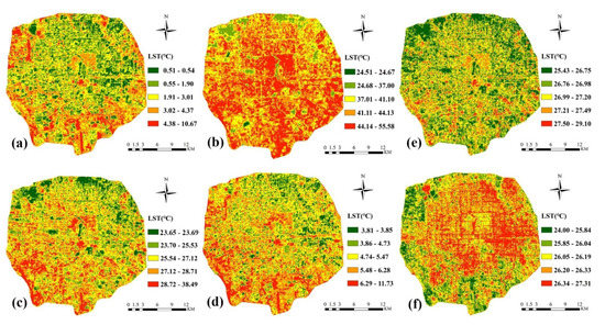
Figure 4.
LST results of the study area: (a) 3 February 2018 based on Landsat-8 data; (b) 27 June 2018 based on Landsat-8 data; (c) 1 October 2018 based on Landsat-8 data, (d) 4 December 2018 based on Landsat-8 data, (e) 5 October day based on ASTER data, (f) 23 September night based on ASTER data.
The average land surface temperatures from Landsat-8 data of area 1, 2, 3 and 4 were 2.34, 1.88, 2.13 and 2.82 °C on 3rd February; 45.25, 43.07, 42.61 and 42.24 °C on 27 June; 26.87, 26.62, 26.72 and 26.55 °C on 1 October; and 5.41, 5.13, 5.15, 5.45 °C on 4 December, respectively.
For analysis of the SVF–LST relationship during daytime and nighttime, we used the land surface temperature product of ASTER_08v003 with a spatial resolution of 90 m, as shown in Figure 4e,f. We explored the effect of nighttime and daytime variation on the SVF–LST relationship; the LST results on 5 October 2020 are shown in Figure 4e and the LST results on 23 September 2018 are shown in Figure 4f.
In order to be able to compare the average temperatures of different study areas in different seasons more clearly, the average temperatures were normalized, where 1 is the highest temperature and 0 is the lowest temperature in each season, as shown in Figure 5.
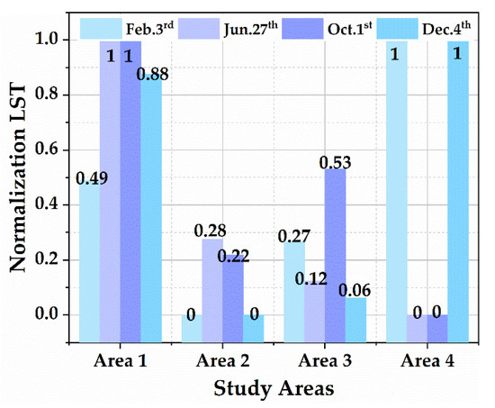
Figure 5.
Land surface temperature distribution based on Landsat-8 data.
It can be seen that the trend of LST changes on 3 February and 4 December are the same, with higher average LST in area 1 and 4, and lower average LST at area 2 and 3; the highest value of average LST on 27 June and 1 October was in area 1, and the lowest value was in area 4, but the average LST on 27 June gradually decreased from area 2 to 4, while on 1st October the temperature in area 3 was higher than that in area 1. It shows that there are differences in the distribution of LST in different seasons and study areas.
The correlation analysis between the retrieved LST and the corresponding SVF using Landsat-8 daily thermal infrared data for 3 February 2018, 27 June 2018, 1 October 2018 and 4 December 2018, in area 1, 2, 3 and 4, is shown in Figure 6, and the R2 of fitting results are shown in Table 2.
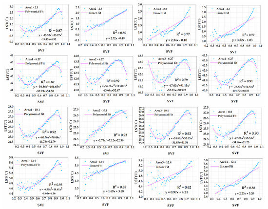
Figure 6.
Relationship between SVF and LST in different study areas and season based on Landsat-8 data.
Table 2.
The R2 of fitting results.
The statistical results of LST and SVF at the four periods show that the trends of the SVF and LST fitting results are the same in different loop regions on 3 February and 4 December, which are nonlinearly correlated in area 1 and positively linearly correlated in the remaining three areas, while the trends of SVF and LST fitting results are similar in different study areas on 27 June and 1 October.
Thus, there is a seasonal difference between SVF and LST. From the above results, we found that the positive correlation between SVF and LST was significant on 3 February and 4 December and that the temperature was cooler on the two periods. This relationship was opposite to the nighttime experiment. The main reason for the results may be that the land surface absorbs more solar radiation than it scatters. Where the SVF is lower, some part of the solar radiation is impeded by the buildings; thus, the LST is lower. In addition, where the SVF is higher, the openness of the areas can absorb solar radiation; therefore, the LST is higher.
Conversely, the SVF–LST relationship is more complex on 27 June and 1 October. The SVF–LST relationship is negatively correlated at the value of SVF at 0 to 0.4 and 0.9 to 1. We thought of SVF at 0 to 0.4 as a low visible region and 0.9 to 1 as high visible region. Considering vegetation, energy consumption of air conditioning, etc. as factors on LST, they are more significant on 27 June and 1 October. The LST reduced the value of SVF from 0 to 0.4. The LST was higher in the areas closer to buildings. That might be due to the heat emission from buildings in high temperature weather. As the distance between buildings increased, the air flow between them was enhanced, allowing the radiation between them to spread. Thus, the LST was lower in the SVF than the SVF at 0.2. Besides, between the buildings, there was vegetation. That might be due to a cooling effect by the air flow and vegetation around the building. In the high visible region, the functionality of this region may be largely in shadow. Therefore, in the high visible region, there is a cooling trend.
3.3. Day–Night Variation of SVF–LST Relationship
For analysis of the SVF–LST relationship on daytime and nighttime, we used the LST product of ASTER_08v003 with a spatial resolution of 90 m and selected the daytime data on 5 October 2020 and the nighttime data on 23 September 2018. The retrieval of LST based on ASTER data is shown in Figure 4e,f. The statistical and fitting results of the nighttime and daytime SVF–LST relationship of the four study areas are shown in Figure 7 and Figure 8.
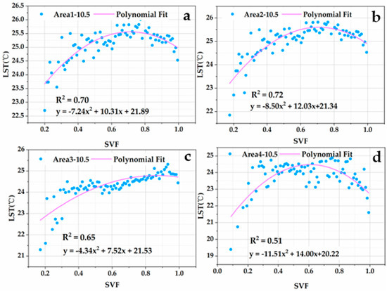
Figure 7.
SVF–LST relationship in different study areas based on ASTER data on 5 October day; (a) area 1; (b) area 2; (c) area 3; (d) area 4.
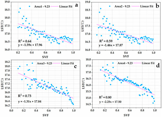
Figure 8.
SVF–LST relationship in different study areas based on ASTER data on 23 September night; (a) area 1; (b) area 2; (c) area 3; (d) area 4.
From Figure 7, we found that there is a non-linear relationship between SVF and LST in daytime. LST first increases and then decreases with an increase of SVF. Then, we calculated the fitted equations of the above statistics and the values of R2, shown in Table 3.
Table 3.
The R2 of fitting results.
Accordingly, the statistical results within the study areas are shown in Figure 8. We found that the SVF and LST are negatively and linearly correlated at nighttime, and the relationship between nighttime LST and SVF on 23 September is also negatively correlated in different areas in terms of the fitting results. Then, we calculated the fitted equations of the above statistics and the values of R2, as shown in Table 3.
From Table 3, we found that the average value of R2 on 23 September 2018 is higher than on 5 October 2020, and this is mainly because less disturbances could lead to the better fitting result in nighttime. At night, due to low sky visibility, the diffusion degree of surface thermal radiation is small; thus, the LST in the areas with low SVF is always high, while, in the area with higher SVF, the LST in this area is relatively lower because the open sky visibility would make enough space for surface thermal radiation diffusion. Therefore, we could see that low SVF and high surface heat storage capacity in the area adjacent to buildings would cause high LST at nighttime.
In the temporal analysis, we found that the SVF–LST relationship is significantly different in daytime and nighttime. The SVF–LST relationship is a significant negative correlation at night. The results show that the LST is lower in the area with higher SVF, and it might be that the main surface radiation processes at night are long-wave radiation emissions, and the area of high SVF with less surrounding obstacles is conducive to the long-wave radiation emission. While in low SVF areas, the long-wave radiation emission would be re-reflected by the walls of the building. This is not conducive to the surface long-wave radiation emission. Therefore, the LST is higher in lower SVF areas. The results are consistent with the findings of Yang [16].
In the daytime, the SVF–LST relationship is non-linear. We found that the LST increases with increasing SVF, where SVF is between 0 and 0.7, which may be because, in the high SVF areas, the surface would absorb more solar short-wave radiation, while the LST decreases with increasing SVF, where SVF is between 0.7 and 1. This is probably because in the high SVF area, even if the absorbed solar radiation is higher, there is less interaction with surrounding objects. Therefore, in high SVF areas, the LST tends to decrease compared to the increased reflected radiation, due to the interactions caused by the surrounding buildings. This is inconsistent with the findings of Zhang [23] in that the SVF–LST relationship is linearly and positively correlated.
The seasonal impact analysis of the SVF–LST relationship is inconsistent with the results of previous studies [18,29]. We found that the SVF–LST relationship is more complex than previous studies. The reasons for this result might be that the Landsat8 data have higher resolution than ASTER data, which can obtain more feature details. Thus, the SVF is in the region of 0–0.4, and the SVF–LST relationship is different between the two types of data. Besides, the reason for this relationship might be the influence of the features around the building on the LST.
3.4. Impact of Building Height and Density on SVF–LST Relationship
The SVF–LST relationship has differences during the daytime. Therefore, in order to analyze the different relationships between LST and SVF in the daytime, different scenes of building morphological features were selected to explore the combined effects of building height, density, SVF and shading on LST at 30 m spatial scale.
We selected three 3D building scenes, which were low-rise buildings with an average number of two floors, multi-story buildings with five floors and mid-rise buildings with seven floors. Because of the height limitation of buildings in the Beijing urban area, the distribution of high-rise buildings is more discrete and not suitable for continuous SVF–LST analysis; thus, the test area of this study does not include high-rise and super high-rise building areas.
In addition, in order to weaken the interference of natural ground surface such as vegetation and water bodies, the three building scenarios were avoided in these areas. The selected building and three-dimensional scenarios used a cesium lab as the test area: area 1 for low-rise buildings located in the northeast of the second ring, area 2 for multi-story buildings located in the northeast between the third and fourth rings, and area 3 for mid- and high-rise buildings located in the southwest between the third and fourth ring roads, as shown in Figure 9.

Figure 9.
Test area with different building heights: (a1,a2) test 1, mean height = 6 m; (b1,b2) test 2, mean height = 15 m; (c1,c2) test 3, mean height = 35 m.
The SVF–LST relationship in the three test areas were analyzed for the degree to which land surface temperature is affected by building height and density. The statistical results are shown in Figure 10. The results indicated that the LST is higher in building heights of 6 m and are lower at 21 m. Although the higher buildings include larger areas of building façades that absorbed more solar radiation, the tall buildings led to more shadow, which may explain why in the higher areas, the LST is higher.
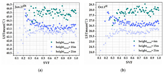
Figure 10.
The SVF–LST relationship with different building heights: (a) test in summer; (b) test in autumn.
In addition, we found the different SVF–LST relationships in three test areas. The most different SVF–LST relationship during the SVF was at 0 to 0.4, which is in the low visual area. This region is closer to buildings and includes the double effect because of the higher buildings and shadow rations, which make the cooling effect more noticeable. The heat storage capacity of the building improved the surrounding thermal environment of the buildings.
The SVF–LST relationship is different in the experiment of different scenes of building morphological features. We guess that there are many factors that lead to the different results in the SVF–LST relationship in the above three building scenes, such as the building shadow ratio, which reduces the LST and is relevant with regard to the height of the building. Conversely, the different building forms lead to different wind environments. However, we do not know the condition to measure the distribution of the wind in the selected building scenes. Therefore, we ignored the effect of a wind field on LST.
3.5. The Relationship between SVF and Building Shadow Ratios
The percentage of building shadows in different visual ranges of the three test areas in different seasons were counted.
First, we used a building vector database with characteristics of building height and solar altitude angle by the geometric position of the building and the sun to extract the building shadow in the three tests. Second, the buildings’ shadow ratio of different SVF intervals was counted. The SVF was divided into 0.1 intervals, and the number of shaded pixels in each interval was calculated, from which the shaded areas of buildings in different visual areas were calculated. The statistical results are shown in Figure 11. We selected summer, autumn and winter as the seasons, and did not select spring because the characteristic of building shadow in spring is not significant. The building shadow and LST data is shown in Table 4.
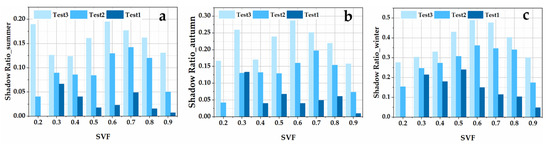
Figure 11.
The relationship between SVF and shade ratio in different seasons: (a) test in summer; (b) test in autumn; (c) test in winter.
Table 4.
Satellite images data information.
With the season change, the building shadow ratio will change because of the change of the solar angle. Therefore, the relationship between SVF and building shadows in three test areas in three seasons were counted separately. The average shading ratio of buildings in summer test areas 1, 2 and 3 were 0.03, 0.1 and 0.16, respectively, in which the shading ratio of mid-rise and multi-story building areas was the largest when SVF was 0.6, while the shading ratio of low-rise building areas was the largest when SVF was 0.3. This indicates that the shading area ratio of buildings increased with SVF when the average height of buildings was higher, and when the SVF reached 0.6, the shaded area of buildings gradually decreased. When the average height of the buildings was low and the density was high, the percentage of shaded area was smaller and the relationship with SVF was not significant. The average shading ratio of the three test areas in autumn was 0.06, 0.13 and 0.22, respectively, which was generally higher than that in summer. The shading ratio of the mid-rise and high-rise building areas was the largest at SVF 0.3 and 0.6, the multi-story building area was the largest at SVF 0.7, and the low-rise building area was the largest at SVF 0.3. The trend of shadow occupancy in the mid-rise and multi-story building areas increases with SVF and decreases after reaching the maximum value, while the low-rise building area decreases with increasing SVF. The statistical results of the three test areas in winter were consistent with each other, and the average shading ratios were 0.15, 0.28 and 0.38, respectively. The shading ratios in the mid-rise and multi-story building areas increased with SVF and decreased gradually when the SVF was 0.6, while the shading ratios in the low-rise building area showed a gradual decrease with an increase of SVF.
From the statistical results of SVF and building shadows in the three experimental areas, as shown in Figure 12, the SVF and shadow ratio are nonlinear when the building height is high, and the shadow ratio reaches a maximum as SVF is 0.6; the LST also decreases in this SVF region.
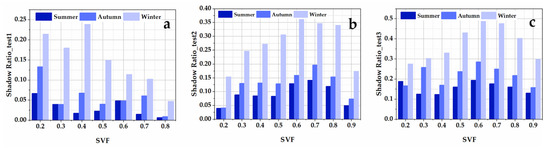
Figure 12.
The relationship between SVF and shade ratio in different test areas: (a) test 1; (b) test 2; (c) test 3.
3.6. Impact of Shadow Rations on LST-SVF Relationship
The building shadow extraction results were correlated, and seasonal differences were analyzed with the LST results at the corresponding time of different SVF intervals.
The average LST in each interval was calculated by dividing the SVF by 0.01, where the spatial resolution was 30 m. The statistical results of the three test areas in different seasons are shown in Figure 13.
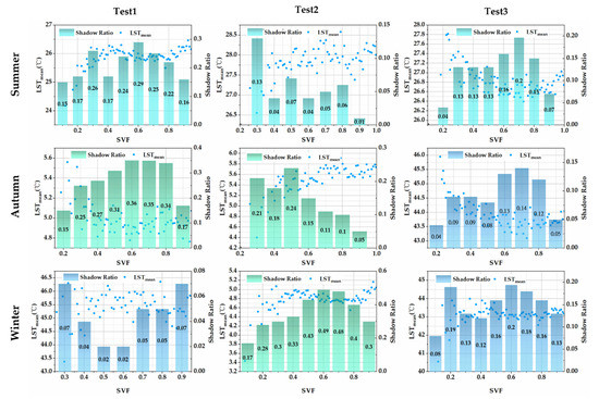
Figure 13.
Shading ratio and the SVF–LST relationship on three tests of different seasons.
The graph of statistical results shows that the consistency of SVF versus LST trends in the three test areas is better in test area 3 than in test areas 2 and 1, with test area 1 having a lower consistency of the correlation results. The average height of the buildings in test area 3 was 21 m. The SVF–LST relationship for all six groups of tests was that LST increased with SVF for the visibility range of 0 to 0.4, decreased with SVF for the visibility range of 0.4 to 0.6, and increased with SVF for the visibility range of 0.6–1. In addition, it can also be seen that the corresponding LST is lower in the areas with higher shadow occupancy, such as SVF in the region of 0.6, where the shadow occupancy is higher in all six groups of the tests, and their LSTs show a decreasing trend. The average height of the buildings in test area 2 is 15 m, which is of multi-story buildings. The statistical results of the six groups of tests show that the SVF–LST relationship is consistent, and the LST gradually decreases in the area where SVF is at 0 to 0.6, while in the area of 0.6 to 1, the LST is a slow and insignificant increasing trend. By comparing the Google Earth high-resolution images, it can be seen that the visible range with SVF values of 0 to 0.6 is mostly distributed in the area close to the buildings, and as the SVF values increase farther away from the buildings, the degree of heat storage decreases, and thus the LST gradually decreases in the area of 0 to 0.6 as the SVF becomes larger. However, the open area of test area 2 is distributed with six larger playgrounds, parking lots, squares, etc., with higher heat storage capacity; thus, the LST slowly increases in the area with SVF of 0.6 to 1. The average height of the buildings in test area 1 is 6 m.
The buildings are characterized by high density and low height. Probably because of the small area of the selected test area and the relatively small sample size for the statistics, the statistical results of the six sets of tests showed that the SVF–LST relationship was not obvious and differed. The SVF–LST relationship was increasing and then decreasing in the summer experiment results, and the relationship between the two in the autumn experiment results was a trend of increasing and then decreasing and then increasing, which was consistent with the results of the statistical relationship between the two in test area 3. The winter experiment results showed a trend of increasing LST with increasing SVF. The statistical results of test area 1 show that there is a seasonal difference between SVF and LST, and building morphology is not the dominant factor affecting LST. Although the main feature in test area 1 is a building, it may be because the building height is low, the degree of influence on LST is low, thus it can also be seen that there is a significant influence of the three-dimensional morphology of the building on the LST distribution.
The statistical results of the nine sets of correlation analysis in the three test areas show that the higher areas of buildings have a more obvious effect on the SVF–LST relationship. In addition, the histogram of the shading ratio of different SVF areas shows that the corresponding LST is lower in the areas with a higher shading ratio; conversely, the LST is higher in the areas with a lower shading ratio. However, the joint influence relationship between SVF and building shadows on LST is not clear.
4. Conclusions
In this paper, we selected the core built-up area of Beijing as the study area to explore the influence of sky view factor on the spatial and temporal distribution of an urban thermal environment. We used daytime and nighttime LST data from ASTER, and analyzed the relationship between LST and SVF. Then, we analyzed the SVF–LST relationship in different seasons by Landsat-8 thermal infrared data.
The results show that SVF and LST are positively correlated at night, and the relationship between them during the daytime varies depending on the image element scale and different seasons, as determined by LST data from ASTER. The nonlinear fitting results of the SVF–LST relationship at the image scale of 30 m are better than those at the image scale of 90 m. Therefore, three types of building scenes with different heights were selected in the study area, and the building shadows in different SVF intervals were counted at an image scale of 30 m. The seasonal differences of the SVF–LST relationship was also analyzed. The results show that the average building shadow ratio in winter was the largest in all three types of scenes, and the shadow ratio of multi-story and mid-rise buildings was the largest when the SVF was 0.6. The SVF was negatively correlated with the shadow ratio in the low-rise building area, while the trend of both increased and decreased in the multi-story and mid-rise building areas. In addition, the LST was lower in the areas with a higher shaded area, and the cooling effect of shading had some influence on the SVF–LST relationship. We found that the fitting results of SVF and LST were more consistent at the same time when the image element scale was 90 m, while the relationship between them differed for building scenes of different heights when the spatial scale was at 30 m. At small scales, more ground information can be obtained than at large scales. Thus, in addition to building morphology, factors such as vegetation, water bodies and anthropogenic heat can also impact the LST distribution, leading to various differences in the SVF–LST relationship.
In this study, we only used the SVF and building shadow ratio to analyze the influence of the 3D structure of buildings on LST in different building scenes. We ignored the interference of vegetation and water while the data were statistically analyzed. However, in different building functions that produce different anthropogenic heat, the environment around the building also affects the surface temperature; thus, further studies should consider the influence of the joint building functional area and the environment around the building on land surface temperature.
Author Contributions
Conceptualization, Q.C. (Qiang Chen) and Y.C.; Methodology, Q.C. (Qianhao Cheng); Software, Q.C. (Qianhao Cheng); Validation, Q.C. (Qiang Chen); Formal Analysis, Q.C. (Qiang Chen) and Y.C.; Investigation, Q.C. (Qianhao Cheng); Data Curation, Q.C. (Qianhao Cheng); Writing—Original Draft Preparation, Q.C. (Qianhao Cheng); Writing—Review and Editing, Q.C. (Qiang Chen), Q.C. (Qianhao Cheng), K.L., D.W., S.C.; Visualization, Q.C. (Qianhao Cheng); Supervision, Q.C. (Qianhao Cheng); Project Administration, Q.C. (Qiang Chen); Funding Acquisition, Q.C. (Qiang Chen). All authors have read and agreed to the published version of the manuscript.
Funding
This work was supported in part by the National Natural Science Foundation of China: 41801235, The Pyramid Talent Training Project of BUCEA: JDYC20200321, Beijing Natural Science Foundation 8192025, BUCEA Post Graduate Innovation Project: 31081021004.
Data Availability Statement
The data that support the findings of this study are available from the author upon reasonable request.
Acknowledgments
The authors would like to thank the editors and anonymous reviewers for their valuable time and efforts in reviewing this manuscript.
Conflicts of Interest
The authors declare no conflict of interest.
Appendix A
Table A1.
The running time of each step of the experiment.
Table A1.
The running time of each step of the experiment.
| Step | Data | Data Size (MB) | Running Time (s) | Software |
|---|---|---|---|---|
| 1. LST retrieval | Landsat-8 TIR | 920 | 60 | ENVI/IDL |
| ASTER | 6 | 30 | ENVI/IDL | |
| 2. SVF calculation | Building Vector | 182 | 150 | ArcGIS, ENVI/IDL |
| 3. SVF–LST analysis | LST retrieval images and SVF images | 11 | 30 | Origin, Matlab |
References
- Xie, M.; Chen, J.; Zhang, Q.; Li, H.; Fu, M.; Breuste, J. Dominant landscape indicators and their dominant areas influencing urban thermal environment based on structural equation model. Ecol. Indic. 2020, 111, 105992. [Google Scholar] [CrossRef]
- Kafy, A.-A.; Islam, M.; Sikdar, S.; Ashrafi, T.J.; Al-Faisal, A.; Islam, M.A.; Al Rakib, A.; Khan, M.H.H.; Sarker, M.H.S.; Ali, M.Y. Remote Sensing-Based Approach to Identify the Influence of Land Use/Land Cover Change on the Urban Thermal Environment: A Case Study in Chattogram City, Bangladesh. In Re-Envisioning Remote Sensing Applications; CRC Press: Boca Raton, FL, USA, 2021; pp. 217–240. [Google Scholar]
- Sharma, R.; Pradhan, L.; Kumari, M.; Bhattacharya, P. Assessing urban heat islands and thermal comfort in Noida City using geospatial technology. Urban Clim. 2021, 35, 100751. [Google Scholar] [CrossRef]
- Makvandi, M.; Zhou, X.; Li, C.; Deng, Q. A Field Investigation on Adaptive Thermal Comfort in an Urban Environment Considering Individuals’ Psychological and Physiological Behaviors in a Cold-Winter of Wuhan. Sustainability 2021, 13, 678. [Google Scholar] [CrossRef]
- Kim, S.W.; Brown, R.D. Urban heat island (UHI) intensity and magnitude estimations: A systematic literature review. Sci. Total Environ. 2021, 779, 146389. [Google Scholar] [CrossRef]
- Delpak, N.; Sajadzadeh, H.; Hasanpourfard, S.; Aram, F. The Effect of Street Orientation on Outdoor Thermal Comfort in a Cold Mountainous Climate. Preprints 2021. [CrossRef]
- Yang, J.; Ren, J.; Sun, D.; Xiao, X.; Xia, J.C.; Jin, C.; Li, X. Understanding land surface temperature impact factors based on local climate zones. Sustain. Cities Soc. 2021, 69, 102818. [Google Scholar] [CrossRef]
- Yang, Z.; Chen, Y.; Zheng, Z.; Huang, Q.; Wu, Z. Application of building geometry indexes to assess the correlation between buildings and air temperature. Build. Environ. 2020, 167, 106477. [Google Scholar] [CrossRef]
- Zhao, C.; Jensen, J.L.; Weng, Q.; Currit, N.; Weaver, R. Use of Local Climate Zones to investigate surface urban heat islands in Texas. GISci. Remote Sens. 2020, 57, 1083–1101. [Google Scholar] [CrossRef]
- Ma, Y.; Zhang, S.; Yang, K.; Li, M. Influence of spatiotemporal pattern changes of impervious surface of urban megaregion on thermal environment: A case study of the Guangdong–Hong Kong–Macao Greater Bay Area of China. Ecol. Indic. 2021, 121, 107106. [Google Scholar] [CrossRef]
- Govind, N.R.; Ramesh, H. The impact of spatiotemporal patterns of land use land cover and land surface temperature on an urban cool island: A case study of Bengaluru. Environ. Monit. Assess. 2019, 191, 283. [Google Scholar] [CrossRef]
- Feng, L.; Zhao, M.; Zhou, Y.; Zhu, L.; Tian, H. The seasonal and annual impacts of landscape patterns on the urban thermal comfort using Landsat. Ecol. Indic. 2020, 110, 105798. [Google Scholar] [CrossRef]
- Alavipanah, S.; Schreyer, J.; Haase, D.; Lakes, T.; Qureshi, S. The effect of multi-dimensional indicators on urban thermal conditions. J. Clean. Prod. 2018, 177, 115–123. [Google Scholar] [CrossRef]
- Guo, J.; Sun, B.; Qin, Z.; Wong, M.S.; Wong, S.W.; Yeung, C.W.; Wang, H.; Sawaid, A.; Shen, G.Q. Analysing the effects for different scenarios on surrounding environment in a high-density city. Cities 2020, 99, 102585. [Google Scholar] [CrossRef]
- Sun, F.; Liu, M.; Wang, Y.; Wang, H.; Che, Y. The effects of 3D architectural patterns on the urban surface temperature at a neighborhood scale: Relative contributions and marginal effects. J. Clean. Prod. 2020, 258, 126702. [Google Scholar] [CrossRef]
- Yang, J.; Menenti, M.; Wu, Z.; Wong, M.S.; Abbas, S.; Xu, Y.; Shi, Q. Assessing the impact of urban geometry on surface urban heat island using complete and nadir temperatures. Int. J. Climatol. 2021, 41, E3219–E3238. [Google Scholar] [CrossRef]
- Liu, Y.; Li, Q.; Yang, L.; Mu, K.; Zhang, M.; Liu, J. Urban heat island effects of various urban morphologies under regional climate conditions. Sci. Total Environ. 2020, 743, 140589. [Google Scholar] [CrossRef]
- Xu, Y.; Ren, C.; Ma, P.; Ho, J.; Wang, W.; Lau, K.K.-L.; Lin, H.; Ng, E. Urban morphology detection and computation for urban climate research. Landsc. Urban Plan. 2017, 167, 212–224. [Google Scholar] [CrossRef]
- Xiao, M.; Lin, Y.; Han, J.; Zhang, G. A review of green roof research and development in China. Renew. Sustain. Energy Rev. 2014, 40, 633–648. [Google Scholar] [CrossRef]
- Chen, Y.; Wu, J.; Yu, K.; Wang, D. Evaluating the impact of the building density and height on the block surface temperature. Build. Environ. 2020, 168, 106493. [Google Scholar] [CrossRef]
- Zheng, Z.; Zhou, W.; Yan, J.; Qian, Y.; Wang, J.; Li, W. The higher, the cooler? Effects of building height on land surface temperatures in residential areas of Beijing. Phys. Chem. Earth Parts A/B/C 2019, 110, 149–156. [Google Scholar] [CrossRef]
- Wang, Y.; Akbari, H. Effect of Sky View Factor on Outdoor Temperature and Comfort in Montreal. Environ. Eng. Ence 2014, 31, 272–287. [Google Scholar] [CrossRef]
- Zhang, J.; Gou, Z.; Lu, Y.; Lin, P. The impact of sky view factor on thermal environments in urban parks in a subtropical coastal city of Australia. Urban For. Urban Green. 2019, 44, 126422. [Google Scholar] [CrossRef]
- Cai, H.; Xu, X. Impacts of built-up area expansion in 2D and 3D on regional surface temperature. Sustainability 2017, 9, 1862. [Google Scholar] [CrossRef] [Green Version]
- Yang, J.; Shi, B.; Xia, G.; Xue, Q.; Cao, S.-J. Impacts of Urban form on Thermal Environment near the Surface Region at Pedestrian Height: A Case Study Based on High-density Built-up Areas of Nanjing City in China. Sustainability 2020, 12, 1737. [Google Scholar] [CrossRef] [Green Version]
- Oke, T.R. Boundary Layer Climates, 2nd ed.; Routledge: London, UK, 2015. [Google Scholar]
- Miao, C.; Yu, S.; Hu, Y.; Zhang, H.; He, X.; Chen, W. Review of methods used to estimate the sky view factor in urban street canyons. Build. Environ. 2020, 168, 106497. [Google Scholar] [CrossRef]
- Zhang, H.L.; Zhu, Y.S.; Gao, Y.; Zhang, G.X. The Relationship Between Urban Spatial Morphology Parameters and Urban Heat Island Intensity Under Fine Weather Condition. J. Appl. Meteorol. Sci. 2016, 27, 249–256. [Google Scholar]
- Scarano, M.; Sobrino, J.A. On the relationship between the sky view factor and the land surface temperature derived by Landsat-8 images in Bari, Italy. Int. J. Remote Sens. 2015, 36, 4820–4835. [Google Scholar] [CrossRef]
- Scarano; Mancini. Assessing the relationship between sky view factor and land surface temperature to the spatial resolution. Int. J. Remote Sens. 2017, 38, 6910–6929. [Google Scholar] [CrossRef]
- Yu, W.; Ma, M.; Yang, H.; Tan, J.; Li, X. Supplement of the radiance-based method to validate satellite-derived land surface temperature products over heterogeneous land surfaces. Remote Sens. Environ. 2019, 230, 111188. [Google Scholar] [CrossRef]
- Qaid, A.; Lamit, H.B.; Ossen, D.R.; Rasidi, M.H. Effect of the position of the visible sky in determining the sky view factor on micrometeorological and human thermal comfort conditions in urban street canyons. Theor. Appl. Climatol. 2018, 131, 1083–1100. [Google Scholar] [CrossRef]
- Zaksek, K.; Oštir, K.; Kokalj, Ž. Sky-View Factor as a Relief Visualization Technique. Remote Sens. 2011, 3, 398. [Google Scholar] [CrossRef] [Green Version]
- Fariza, A.; Basofi, A.; Aryani, M. Spatial mapping of diphtheria vulnerability level in East Java, Indonesia, using analytical hierarchy process–natural break classification. In Proceedings of the Journal of Physics: Conference Series; IOP Publishing: Bristol, UK, 2021; p. 012009. [Google Scholar]
Publisher’s Note: MDPI stays neutral with regard to jurisdictional claims in published maps and institutional affiliations. |
© 2021 by the authors. Licensee MDPI, Basel, Switzerland. This article is an open access article distributed under the terms and conditions of the Creative Commons Attribution (CC BY) license (https://creativecommons.org/licenses/by/4.0/).