
Remote Sensing of Local Warming Trend in Alberta, Canada during 2001–2020, and Its Relationship with Large-Scale Atmospheric Circulations

 ,
,  , ,
, , 
Abstract
:1. Introduction
2. Study Area and Data Used
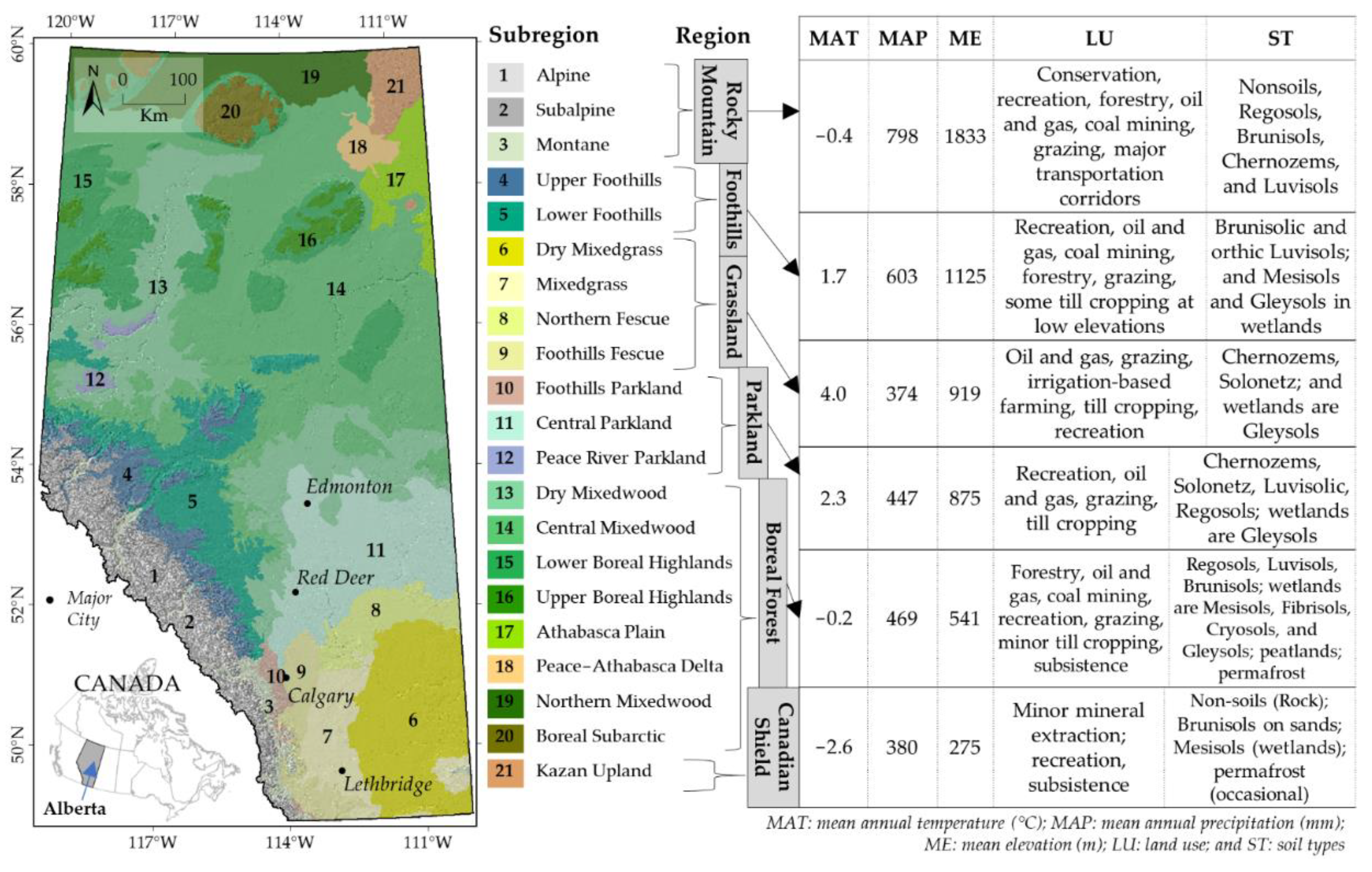
2.1. Description of the Study Area
2.2. Data Used and Their Preprocessing
3. Methods
3.1. Mapping Local Warming Trend
3.1.1. Mann–Kendall Test
3.1.2. Sen’s Slope Estimator
3.2. Correlating Atmospheric Oscillations
4. Results
4.1. Analysis of Local Warming Trend at the Natural Subregion Scale
4.2. Correlation Analysis of LST Anomalies with the Atmospheric Oscillations
5. Discussion
6. Conclusions
Author Contributions
Funding
Acknowledgments
Conflicts of Interest
References
- Jones, P.D.; Lister, D.H.; Osborn, T.J.; Harpham, C.; Salmon, M.; Morice, C.P. Hemispheric and large-scale land-surface air temperature variations: An extensive revision and an update to 2010. J. Geophys. Res. Atmos. 2012, 117. [Google Scholar] [CrossRef] [Green Version]
- Ji, F.; Wu, Z.; Huang, J.; Chassignet, E.P. Evolution of Land Surface Air Temperature Trend. Nat. Clim. Chang. 2014, 4, 462–466. [Google Scholar] [CrossRef]
- Routson, C.C.; Nicholas, P.; Kaufman, D.S.; Michael, P.; Goosse, H.; Shuman, B.N.; Rodysill, J.R.; Ault, T. Mid-latitude net precipitation decreased with Arctic warming during the Holocene. Nature 2019, 568, 83–87. [Google Scholar] [CrossRef] [PubMed]
- Serreze, M.C.; Barry, R.G. Processes and impacts of Arctic amplification: A research synthesis. Glob. Planet. Chang. 2011, 77, 85–96. [Google Scholar] [CrossRef]
- Bush, E.; Lemmen, D.S. (Eds.) Canada’s Changing Climate Report; Government of Canada: Ottawa, ON, Canada, 2019.
- IPCC 2013. Climate Change 2013: The Physical Science Basis. Working Group I Contribution to the Fifth Assessment Report of the Intergovernmental Panel on Climate Change; Stocker, T.F., Qin, D., Plattner, G.K., Tignor, M.M.B., Allen, S.K., Boschung, J., Nauels, A., Xia, Y., Bex, V., Midgley, P.M., Eds.; Cambridge University Press: Cambridge, UK; New York, NY, USA, 2013; Volume 9781107057, ISBN 9781107415324. [Google Scholar]
- McCarthy, M.P.; Best, M.J.; Betts, R.A. Climate change in cities due to global warming and urban effects. Geophys. Res. Lett. 2010, 37. [Google Scholar] [CrossRef] [Green Version]
- Rahaman, K.R.; Hassan, Q.K.; Chowdhury, E.H. Quantification of Local Warming Trend: A Remote Sensing-Based Approach. PLoS ONE 2017, 12, e0196882. [Google Scholar] [CrossRef]
- Yan, Y.; Mao, K.; Shi, J.; Piao, S.; Shen, X.; Dozier, J.; Liu, Y.; Ren, H.-l.; Bao, Q. Driving forces of land surface temperature anomalous changes in North America in 2002–2018. Sci. Rep. 2020, 10, 6931. [Google Scholar] [CrossRef]
- Lynch, M.; Evans, A. 2017 Wildfire Season: An Overview, Southwestern U.S. Special Report; Ecological Restoration Institute and Southwest Fire Science Consortium, Northern Arizona University: Flagstaff, AZ, USA, 2018. [Google Scholar]
- Menne, M.J.; Williams, C.N.; Palecki, M.A. On the reliability of the U.S. surface temperature record. J. Geophys. Res. 2010, 115. [Google Scholar] [CrossRef] [Green Version]
- Mahlstein, I.; Hegerl, G.; Solomon, S. Emerging local warming signals in observational data. Geophys. Res. Lett. 2012, 39. [Google Scholar] [CrossRef]
- Maduako, I.N.; Ebinne, E.; Idorenyin, U.; Ndukwu, R.I. Accuracy Assessment and Comparative Analysis of IDW, Spline and Kriging in Spatial Interpolation of Landform (Topography): An Experimental Study. J. Geogr. Inf. Syst. 2017, 9, 354–371. [Google Scholar] [CrossRef] [Green Version]
- Bhunia, G.S.; Shit, P.K.; Maiti, R. Comparison of GIS-based interpolation methods for spatial distribution of soil organic carbon (SOC). J. Saudi Soc. Agric. Sci. 2018, 17, 114–126. [Google Scholar] [CrossRef] [Green Version]
- Ahmed, M.R.; Hassan, Q.K.; Abdollahi, M.; Gupta, A. Introducing a new remote sensing-based model for forecasting forest fire danger conditions at a four-day scale. Remote Sens. 2019, 11, 2101. [Google Scholar] [CrossRef] [Green Version]
- Akbar, T.A.; Hassan, Q.K.; Ishaq, S.; Batool, M.; Butt, H.J.; Jabbar, H. Investigative Spatial Distribution and Modelling of Existing and Future Urban Land Changes and Its Impact on Urbanization and Economy. Remote Sens. 2019, 11, 105. [Google Scholar] [CrossRef] [Green Version]
- Luintel, N.; Ma, W.; Ma, Y.; Wang, B.; Subba, S. Spatial and temporal variation of daytime and nighttime MODIS land surface temperature across Nepal. Atmos. Ocean. Sci. Lett. 2019, 12, 305–312. [Google Scholar] [CrossRef] [Green Version]
- Olivares-Contreras, V.A.; Mattar, C.; Gutiérrez, A.G.; Jiménez, J.C. Warming trends in Patagonian subantartic forest. Int. J. Appl. Earth Obs. Geoinf. 2019, 76, 51–65. [Google Scholar] [CrossRef]
- Jiménez-Muñoz, J.C.; Sobrino, J.A.; Mattar, C.; Malhi, Y. Spatial and temporal patterns of the recent warming of the Amazon forest. J. Geophys. Res. Atmos. 2013, 118, 5204–5215. [Google Scholar] [CrossRef]
- Aguilar-Lome, J.; Espinoza-Villar, R.; Espinoza, J.C.; Rojas-Acuña, J.; Willems, B.L.; Leyva-Molina, W.M. Elevation-dependent warming of land surface temperatures in the Andes assessed using MODIS LST time series (2000–2017). Int. J. Appl. Earth Obs. Geoinf. 2019, 77, 119–128. [Google Scholar] [CrossRef]
- Qie, Y.; Wang, N.; Wu, Y.; Chen, A. Variations in winter surface temperature of the Purog Kangri Ice Field, Qinghai-Tibetan Plateau, 2001-2018, using MODIS data. Remote Sens. 2020, 12, 1133. [Google Scholar] [CrossRef] [Green Version]
- Fallah Ghalhari, G.; Khoshhal Dastjerdi, J.; Habibi Nokhandan, M. Using Mann Kendal and t-test methods in identifying trends of climatic elements: A case study of northern parts of Iran. Manag. Sci. Lett. 2012, 2, 911–920. [Google Scholar] [CrossRef]
- Gocic, M.; Trajkovic, S. Analysis of changes in meteorological variables using Mann-Kendall and Sen’s slope estimator statistical tests in Serbia. Glob. Planet. Chang. 2013, 100, 172–182. [Google Scholar] [CrossRef]
- Rahman, A.-U.; Dawood, M. Spatio-statistical analysis of temperature fluctuation using Mann–Kendall and Sen’s slope approach. Clim. Dyn. 2017, 48, 783–797. [Google Scholar] [CrossRef]
- Li, Y.; Wang, L.; Zhang, L.; Wang, Q. Monitoring the Interannual Spatiotemporal Changes in the Land Surface Thermal Environment in Both Urban and Rural Regions from 2003 to 2013 in China Based on Remote Sensing. Adv. Meteorol. 2019, 2019, 1–17. [Google Scholar] [CrossRef] [Green Version]
- Muster, S.; Langer, M.; Abnizova, A.; Young, K.L.; Boike, J. Spatio-temporal sensitivity of MODIS land surface temperature anomalies indicates high potential for large-scale land cover change detection in Arctic permafrost landscapes. Remote Sens. Environ. 2015, 168, 1–12. [Google Scholar] [CrossRef] [Green Version]
- Ejiagha, I.R.; Ahmed, M.R.; Hassan, Q.K.; Dewan, A.; Gupta, A.; Rangelova, E. Use of Remote Sensing in Comprehending the Influence of Urban Landscape’s Composition and Configuration on Land Surface Temperature at Neighbourhood Scale. Remote Sens. 2020, 12, 2508. [Google Scholar] [CrossRef]
- Pepin, N.; Deng, H.; Zhang, H.; Zhang, F.; Kang, S.; Yao, T. An Examination of Temperature Trends at High Elevations Across the Tibetan Plateau: The Use of MODIS LST to Understand Patterns of Elevation-Dependent Warming. J. Geophys. Res. Atmos. 2019, 124, 5738–5756. [Google Scholar] [CrossRef] [Green Version]
- Harris, P.P.; Huntingford, C.; Cox, P.M. Amazon Basin climate under global warming: The role of the sea surface temperature. Philos. Trans. R. Soc. B Biol. Sci. 2008, 363, 1753–1759. [Google Scholar] [CrossRef] [Green Version]
- Pepin, N.; Bradley, R.S.; Diaz, H.F.; Baraer, M.; Caceres, E.B.; Forsythe, N.; Fowler, H.; Greenwood, G.; Hashmi, M.Z.; Liu, X.D.; et al. Elevation-dependent warming in mountain regions of the world. Nat. Clim. Chang. 2015, 5, 424–430. [Google Scholar] [CrossRef] [Green Version]
- Hall, D.K.; Williams, R.S.; Luthcke, S.B.; Digirolamo, N.E. Greenland ice sheet surface temperature, melt and mass loss: 2000–2006. J. Glaciol. 2008, 54, 81–93. [Google Scholar] [CrossRef] [Green Version]
- Shabbar, A.; Khandekar, M. The impact of el Nino-Southern oscillation on the temperature field over Canada: Research note. Atmos.-Ocean 1996, 34, 401–416. [Google Scholar] [CrossRef]
- Bonsal, B.; Shabbar, A. Large-Scale Climate Oscillations Influencing Canada, 1900-2008; Canadian Biodiversity: Ecosystem Status and Trends 2010. Technical Thematic Report No. 4; Canadian Councils of Resource Ministers: Ottawa, ON, USA,, 2011; 20p.
- Slonosky, V.C.; Jones, P.D.; Davies, T.D. Impacts of low frequency variability modes on Canadian winter temperature. Int. J. Climatol. 2001, 21, 95–108. [Google Scholar] [CrossRef]
- Chen, Z.; Gan, B.; Wu, L.; Jia, F. Pacific-North American teleconnection and North Pacific Oscillation: Historical simulation and future projection in CMIP5 models. Clim. Dyn. 2018, 50, 4379–4403. [Google Scholar] [CrossRef] [Green Version]
- Rafferty, J.P. North Atlantic Oscillation (Climatology). Available online: https://www.britannica.com/science/North-Atlantic-Oscillation (accessed on 22 June 2021).
- Statistics Canada. 2001 Census: Alberta Population. Available online: https://www12.statcan.gc.ca/English/profil01/CP01/Details/Page.cfm?Lang=E&Geo1=CMA&Code1=835__&Geo2=PR&Code2=48&Data=Count&SearchText=Edmonton&SearchType=Begins&SearchPR=01&B1=Population&Custom= (accessed on 14 June 2021).
- Statistics Canada. Census Profile, 2016 Census: Alberta. Available online: https://www12.statcan.gc.ca/census-recensement/2016/dp-pd/prof/details/page.cfm?Lang=E&Geo1=PR&Code1=48&Geo2=PR&Code2=01&SearchText=Alberta&SearchType=Begins&SearchPR=01&B1=Population&TABID=1&type=0 (accessed on 14 June 2021).
- Government of Alberta. Population Statistics: Alberta population Estimates. Available online: https://www.alberta.ca/population-statistics.aspx (accessed on 14 June 2021).
- Government of Alberta. Alberta Population Estimates-Data Tables. Municipal (Census Subdivision) Population Estimates: 2016–2020 (updated 23 March 2021). Available online: https://open.alberta.ca/dataset/alberta-population-estimates-data-tables (accessed on 14 June 2021).
- Natural Regions Committee 2006. Natural Regions and Subregions of Alberta; Downing, D.J., Pettapiece, W.W., Eds.; Government of Alberta: Edmonton, AL, Canada, 2006.
- Achuff, P.L. Natural Regions, Subregions and Natural History Themes of Alberta: A Classification for Protected Areas Management; Alberta Environmental Protection: Edmonton, AL, Canada, 1994. [Google Scholar]
- Marshall, I.B.; Smith, S.C.A.; Selby, C.J. A national framework for monitoring and reporting on environmental sustainability in Canada. Environ. Monit. Assess. 1996, 39, 25–38. [Google Scholar] [CrossRef] [PubMed]
- Mann, H.B. Nonparametric Tests Against Trend. Econometrica 1945, 13, 15. [Google Scholar] [CrossRef]
- Kendall, M.G. Rank Correlation Methods. J. R. Stat. Soc. Ser. D. Stat. 1971, 20, 74. [Google Scholar] [CrossRef]
- Sen, P.K. Estimates of the Regression Coefficient Based on Kendall’s Tau. J. Am. Stat. Assoc. 1968, 63, 1379–1389. [Google Scholar] [CrossRef]
- Nunifu, T.; Long, F. Methods and Procedures for Trend Analysis of Air QUality Data; Government of Alberta, Ministry of Environment and Parks: Edmonton, AL, Canada, 2019; ISBN 978-1-4601-3637-9.
- Kocsis, T.; Kovács-Székely, I.; Anda, A. Comparison of parametric and non-parametric time-series analysis methods on a long-term meteorological data set. Cent. Eur. Geol. 2017, 60, 316–332. [Google Scholar] [CrossRef]
- Hirsch, R.M.; Slack, J.R.; Smith, R.A. Techniques of trend analysis for monthly water quality data. Water Resour. Res. 1982, 18, 107–121. [Google Scholar] [CrossRef] [Green Version]
- Wang, Z.; Lu, Z.; Cui, G. Spatiotemporal variation of land surface temperature and vegetation in response to climate change based on NOAA-AVHRR data over China. Sustainability 2020, 12, 3601. [Google Scholar] [CrossRef]
- Gilewski, P.; Nawalany, M. Inter-comparison of Rain-Gauge, Radar, and Satellite (IMERG GPM) precipitation estimates performance for rainfall-runoff modeling in a mountainous catchment in Poland. Water 2018, 10, 1665. [Google Scholar] [CrossRef] [Green Version]
- Rauf, A.U.; Ghumman, A.R. Impact assessment of rainfall-runoffsimulations on the flow duration curve of the Upper Indus river-a comparison of data-driven and hydrologic models. Water 2018, 10, 876. [Google Scholar] [CrossRef] [Green Version]
- Ommanney, C.S.L. Glaciers of the Canadian Rockies. In Satellite Image Atlas of the Glaciers of the World—North America; Williams, R.S., Jr., Ferrignod, J.G., Eds.; U.S. Geological Survey: Reston, VA, USA, 2002; pp. J199–J289. [Google Scholar]
- Rangwala, I.; Miller, J.R. Climate change in mountains: A review of elevation-dependent warming and its possible causes. Clim. Chang. 2012, 114, 527–547. [Google Scholar] [CrossRef]
- Beniston, M.; Diaz, H.F.; Bradley, R.S. Climatic change at high elevation sites: An overview. Clim. Chang. 1997, 36, 233–251. [Google Scholar] [CrossRef]
- Messerli, B.; Ives, J.D. Mountains of the World: A Global Priority; The Parthenon Publishing Group: New York, NY, USA, 1997. [Google Scholar]
- Vuille, M.; Franquist, E.; Garreaud, R.; Casimiro, W.S.L.; Cáceres, B. Impact of the global warming hiatus on Andean temperature. J. Geophys. Res. Atmos. 2015, 120, 3745–3757. [Google Scholar] [CrossRef] [Green Version]
- Bonsal, B.R.; Prowse, T.D. Trends and variability in spring and autumn 0°C-isotherm dates over Canada. Clim. Chang. 2003, 57, 341–358. [Google Scholar] [CrossRef]
- Schwartz, M.D.; Ahas, R.; Aasa, A. Onset of spring starting earlier across the Northern Hemisphere. Glob. Chang. Biol. 2006, 12, 343–351. [Google Scholar] [CrossRef]
- Burn, D.H. Climatic influences on streamflow timing in the headwaters of the Mackenzie River Basin. J. Hydrol. 2008, 352, 225–238. [Google Scholar] [CrossRef]
- Stewart, I.T.; Cayan, D.R.; Dettinger, M.D. Changes toward earlier streamflow timing across western North America. J. Clim. 2005, 18, 1136–1155. [Google Scholar] [CrossRef]
- Deng, G.; Zhang, H.; Guo, X.; Shan, Y.; Ying, H.; Rihan, W.; Li, H.; Han, Y. Asymmetric Effects of Daytime and Nighttime Warming on Boreal Forest Spring Phenology. Remote Sens. 2019, 11, 1651. [Google Scholar] [CrossRef] [Green Version]
- Van Der Velde, R.; Su, Z.; Ek, M.; Rodell, M.; Ma, Y. Influence of thermodynamic soil and vegetation parameterizations on the simulation of soil temperature states and surface fluxes by the Noah LSM over a Tibetan plateau site. Hydrol. Earth Syst. Sci. 2009, 13, 759–777. [Google Scholar] [CrossRef] [Green Version]
- Peters-Lidard, C.D.; Blackburn, E.; Liang, X.; Wood, E.F. The effect of soil thermal conductivity parameterization on surface energy fluxes and temperatures. J. Atmos. Sci. 1998, 55, 1209–1224. [Google Scholar] [CrossRef]
- Government of Alberta. Alberta Agriculture and Forestry. Alberta Irrigation Information 2019; Lethbridge: Edmonton, AL, Canada, 2020; 34p.
- Shen, S.S. An Assessment of the Change in Temperature and Precipitation in Alberta; Science and Technology Branch, Environmental Sciences Division, Alberta Environment: Edmonton, AL, Canada, 1999. [Google Scholar]
- Liu, T.; Yu, L.; Zhang, S. Land Surface Temperature Response to Irrigated Paddy Field Expansion: A Case Study of Semi-arid Western Jilin Province, China. Sci. Rep. 2019, 9, 5278. [Google Scholar] [CrossRef]
- Yang, Q.; Huang, X.; Tang, Q. Irrigation cooling effect on land surface temperature across China based on satellite observations. Sci. Total Environ. 2020, 705, 135984. [Google Scholar] [CrossRef] [PubMed]
- Gan, T.Y. Hydroclimatic trends and possible climatic warming in the Canadian Prairies. Water Resour. Res. 1998, 34, 3009–3015. [Google Scholar] [CrossRef]
- Chaikowsky, C. Analysis of Alberta Temperature Observations and Estimates by Global Climate Models; Environmental Sciences Division, Alberta Environment: Edmonton, AL, Canada, 2000. [Google Scholar]
- Newton, B.W.; Farjad, B.; Orwin, J.F. Spatial and temporal shifts in historic and future temperature and precipitation patterns related to snow accumulation and melt regimes in Alberta, Canada. Water 2021, 13, 1013. [Google Scholar] [CrossRef]
- Isaac, G.A.; Stuart, R.A. Temperature–Precipitation Relationships for Canadian Stations. J. Clim. 1992, 5, 822–830. [Google Scholar] [CrossRef] [Green Version]
- Liu, Z.; Yoshmura, K.; Bowen, G.J.; Welker, J.M. Pacific-North American teleconnection controls on precipitation isotopes (δ18O) across the Contiguous United States and Adjacent Regions: A GCM-based analysis. J. Clim. 2014, 27, 1046–1061. [Google Scholar] [CrossRef]
- NOAA. National Centers for Environmental Information. Equatorial Pacific Sea Surface Temperatures. Available online: https://www.ncdc.noaa.gov/teleconnections/enso/indicators/sst/ (accessed on 15 July 2021).
- Mantua, N.J.; Hare, S.R.; Zhang, Y.; Wallace, J.M.; Francis, R.C. A Pacific Interdecadal Climate Oscillation with Impacts on Salmon Production. Bull. Am. Meteorol. Soc. 1997, 78, 1069–1079. [Google Scholar] [CrossRef]
- Wu, A.; Hsieh, W.W.; Shabbar, A.; Boer, G.J.; Zwiers, F.W. The nonlinear association between the Arctic Oscillation and North American winter climate. Clim. Dyn. 2006, 26, 865–879. [Google Scholar] [CrossRef]


| Natural Region | Natural Subregion | Month | Annual | |||||||||||
|---|---|---|---|---|---|---|---|---|---|---|---|---|---|---|
| Jan | Feb | Mar | Apr | May | Jun | Jul | Aug | Sep | Oct | Nov | Dec | |||
| Rocky Mountain | Alpine | −0.018 | −0.162 | 0.020 | −0.025 | 0.163 ^ | −0.025 | −0.023 | 0.011 | 0.047 | −0.047 | −0.009 | 0.036 | −0.008 |
| Subalpine | −0.005 | −0.163 | −0.008 | −0.020 | 0.162 | −0.046 | −0.020 | 0.035 | 0.024 | −0.067 | −0.048 | 0.038 | −0.018 | |
| Montane | −0.074 | −0.107 | −0.199 | −0.111 | 0.054 | −0.064 | −0.081 | 0.028 | −0.012 | −0.130 | −0.192 | 0.033 | −0.066 * | |
| Foothills | Upper Foothills | −0.020 | −0.222 | −0.044 | −0.062 | 0.166 * | −0.023 | −0.038 | 0.029 | 0.045 | −0.049 | −0.185 | 0.070 | −0.023 |
| Lower Foothills | −0.010 | −0.172 | −0.020 | −0.129 | 0.189 * | −0.031 | −0.060 | −0.010 | 0.044 | 0.008 | −0.260 | 0.113 | −0.037 | |
| Grassland | Dry Mixedgrass | −0.081 | −0.119 | −0.023 | −0.271 | 0.045 | 0.046 | −0.226 ^ | 0.050 | 0.025 | −0.127 | −0.311 ^ | −0.007 | −0.088 |
| Mixedgrass | −0.085 | −0.173 | −0.084 | −0.186 | 0.027 | −0.040 | −0.190 | 0.061 | 0.092 | −0.179 | −0.344 ^ | −0.003 | −0.111 ^ | |
| Northern Fescue | −0.043 | −0.094 | −0.007 | −0.308 * | 0.007 | −0.064 | −0.341 * | −0.157 | −0.082 | −0.046 | −0.310 | 0.007 * | −0.142 ** | |
| Foothills Fescue | −0.085 | −0.130 | −0.128 | −0.167 | 0.090 | −0.057 | −0.142 ** | 0.020 | 0.031 | −0.149 | −0.360 * | −0.065 | −0.120 * | |
| Parkland | Foothills Parkland | −0.183 | −0.122 | −0.143 | −0.066 | 0.089 | −0.046 | −0.108 ^ | −0.009 | −0.013 | −0.146 | −0.258 | −0.017 | −0.093 ^ |
| Central Parkland | −0.004 | −0.108 | 0.030 | −0.246 | 0.003 | −0.066 | −0.198 * | −0.204 * | −0.077 | −0.044 | −0.278 | 0.034 | −0.126 * | |
| Peace River Parkland | 0.059 | −0.015 | 0.001 | −0.037 | 0.245 * | −0.117 | −0.126 | −0.097 | 0.008 | −0.012 | −0.368 * | 0.186 | −0.023 | |
| Boreal Forest | Dry Mixedwood | 0.068 | −0.092 | −0.016 | −0.153 | 0.163 * | −0.025 | −0.128 | −0.038 | −0.011 | −0.058 | −0.273 ^ | 0.151 | −0.052 |
| Central Mixedwood | 0.056 | −0.147 | 0.044 | −0.117 | 0.154 * | 0.024 | −0.046 | 0.051 | 0.001 | −0.109 | −0.202 | 0.052 | 0.001 | |
| Lower Boreal Highlands | 0.017 | −0.203 | 0.058 | −0.138 | 0.214 * | 0.010 | −0.019 | 0.043 | −0.084 | −0.068 | −0.154 | 0.047 | 0.005 | |
| Upper Boreal Highlands | 0.099 | −0.133 | 0.031 | −0.087 | 0.189 * | 0.024 | 0.007 | 0.064 | 0.019 | −0.112 | −0.230 | 0.015 | 0.000 | |
| Athabasca Plain | 0.029 | −0.208 | −0.009 | 0.035 | 0.320 * | 0.108 | 0.030 | 0.199 * | −0.032 | −0.155 | −0.219 | −0.134 | −0.006 | |
| Peace–Athabasca Delta | 0.003 | −0.128 | 0.037 | 0.051 | 0.240 * | 0.000 | −0.026 | 0.107 | 0.000 | −0.170 | −0.212 | −0.123 | −0.017 | |
| Northern Mixedwood | 0.028 | −0.162 | 0.057 | −0.013 | 0.248 * | 0.080 * | 0.039 | 0.106 | 0.014 | −0.097 | −0.128 | −0.004 | 0.026 | |
| Boreal Subarctic | 0.109 | −0.154 | 0.052 | 0.046 | 0.225 * | 0.036 | −0.035 | 0.051 | 0.043 | −0.086 | −0.103 | −0.032 | 0.022 | |
| Canadian Shield | Kazan Upland | 0.011 | −0.097 | −0.017 | −0.016 | 0.230 * | −0.015 | −0.005 | 0.116 | −0.024 | −0.185 | −0.110 | −0.029 | −0.013 |
| Alberta (Study area) | −0.026 | −0.127 | 0.038 | −0.131 | 0.141 * | 0.004 | −0.079 | 0.002 | −0.004 | −0.047 | −0.219 | 0.044 | −0.032 | |
| Natural Region | Natural Subregion | Month | Annual | |||||||||||
|---|---|---|---|---|---|---|---|---|---|---|---|---|---|---|
| Jan | Feb | Mar | Apr | May | Jun | Jul | Aug | Sep | Oct | Nov | Dec | |||
| Rocky Mountain | Alpine | 0.053 | −0.117 | 0.027 | −0.013 | 0.190 * | 0.019 | 0.013 | 0.060 | 0.013 | −0.050 | −0.023 | −0.003 | 0.013 |
| Subalpine | 0.029 | −0.120 | 0.019 | −0.003 | 0.172 * | −0.008 | −0.013 | 0.085 | 0.023 | −0.049 | −0.026 | −0.011 | 0.008 | |
| Montane | 0.022 | −0.072 | −0.104 | −0.067 | 0.049 | 0.042 | −0.044 | 0.095 ^ | 0.020 | −0.047 | −0.103 | 0.056 | 0.002 | |
| Foothills | Upper Foothills | −0.022 | −0.255 | −0.064 | −0.074 | 0.136 * | 0.027 | −0.017 | 0.059 | 0.030 | −0.075 | −0.139 | 0.047 | −0.027 |
| Lower Foothills | 0.018 | −0.211 | −0.045 | −0.097 | 0.118 * | 0.033 | −0.004 | 0.056 | 0.006 | −0.070 | −0.193 | 0.023 | −0.021 | |
| Grassland | Dry Mixedgrass | −0.089 | −0.050 | −0.134 | −0.136 | −0.013 | 0.027 | −0.058 | 0.075 | 0.007 | −0.150 ^ | −0.188 * | −0.005 | −0.041 |
| Mixedgrass | −0.024 | −0.073 | −0.140 | −0.075 | 0.000 | 0.042 | −0.038 | 0.089 ^ | 0.026 | −0.108 | −0.102 | 0.032 | −0.017 | |
| Northern Fescue | 0.037 | −0.155 | −0.069 | −0.143 | 0.014 | 0.030 | −0.014 | 0.063 | −0.007 | −0.074 | −0.252 ^ | 0.013 | −0.056 | |
| Foothills Fescue | −0.018 | −0.124 | −0.124 | −0.095 | −0.007 | 0.034 | −0.032 | 0.082 * | 0.043 | −0.092 | −0.105 | 0.074 | −0.022 | |
| Parkland | Foothills Parkland | −0.029 | −0.118 | −0.094 | −0.091 | 0.010 | 0.051 | −0.019 | 0.091 * | 0.062 | −0.070 | −0.100 | 0.034 | −0.020 |
| Central Parkland | 0.042 | −0.176 | −0.022 | −0.107 | 0.093 | 0.073 | 0.007 | 0.071 * | 0.053 | −0.052 | −0.253 | 0.098 | −0.040 | |
| Peace River Parkland | 0.032 | −0.130 | −0.053 | −0.031 | 0.182 * | 0.018 | −0.022 | 0.078 | 0.026 | −0.084 | −0.197 | 0.037 | −0.007 | |
| Boreal Forest | Dry Mixedwood | 0.007 | −0.232 | −0.007 | −0.145 | 0.149 * | 0.051 | −0.001 | 0.060 | −0.040 | −0.082 | −0.200 | 0.107 | −0.041 |
| Central Mixedwood | 0.062 | −0.053 | 0.045 | −0.111 | 0.139 ^ | 0.038 | 0.012 | 0.105 | 0.039 | −0.065 | −0.210 | 0.040 | −0.021 | |
| Lower Boreal Highlands | 0.125 | −0.098 | 0.049 | −0.072 | 0.188 ** | 0.031 | 0.018 | 0.099 | 0.034 | −0.079 | −0.244 | 0.078 | −0.013 | |
| Upper Boreal Highlands | 0.109 | −0.085 | 0.004 | −0.060 | 0.186 * | 0.053 | 0.021 | 0.079 | 0.036 | −0.077 | −0.244 | 0.049 | −0.012 | |
| Athabasca Plain | −0.006 | −0.108 | 0.001 | −0.109 | 0.151 | 0.069 | 0.016 | 0.059 | 0.049 | −0.097 | −0.189 | −0.113 | −0.031 | |
| Peace–Athabasca Delta | 0.088 | −0.082 | 0.009 | −0.086 | 0.164 ^ | 0.094 | 0.033 | 0.137 ^ | 0.075 | −0.101 | −0.199 | −0.089 | 0.001 | |
| Northern Mixedwood | 0.058 | −0.101 | 0.043 | −0.123 | 0.134 * | 0.038 | −0.022 | 0.119 | 0.030 | −0.064 | −0.200 ^ | 0.047 | −0.009 | |
| Boreal Subarctic | 0.095 | −0.089 | 0.106 | −0.100 | 0.157 * | 0.040 | −0.014 | 0.095 | 0.036 | −0.034 | −0.219 | 0.058 | −0.002 | |
| Canadian Shield | Kazan Upland | 0.057 | −0.099 | −0.007 | −0.116 | 0.149 | 0.052 | −0.001 | 0.063 | 0.001 | −0.137 | −0.151 | −0.086 | −0.026 |
| Alberta (Study area) | 0.010 | −0.097 | −0.020 | −0.087 | 0.114 ^ | 0.050 | −0.002 | 0.085 | 0.031 | −0.085 | −0.197 | 0.039 | −0.028 | |
| LST | Confidence Level (%) | Area Coverage (%) | |||||||||||||
|---|---|---|---|---|---|---|---|---|---|---|---|---|---|---|---|
| Jan | Feb | Mar | Apr | May | Jun | Jul | Aug | Sep | Oct | Nov | Dec | Annual | |||
| Day | Not significant | 98.72 | 97.24 | 99.71 | 94.15 | 53.21 | 87.62 | 77.13 | 83.09 | 99.90 | 97.77 | 76.59 | 99.98 | 78.98 | |
| Cooling | ≥90 | 0.21 | 2.19 | 0.22 | 4.08 | 0.04 | 2.57 | 8.65 | 2.95 | 0.07 | 1.78 | 16.86 | 0.01 | 7.61 | |
| ≥95 | 0.02 | 0.56 | 0.04 | 1.71 | 0.00 | 1.59 | 10.20 | 4.31 | 0.01 | 0.43 | 6.44 | 0.00 | 10.12 | ||
| ≥99 | 0.00 | 0.01 | 0.00 | 0.06 | 0.00 | 0.33 | 2.38 | 2.21 | 0.00 | 0.01 | 0.11 | 0.00 | 2.81 | ||
| Warming | ≥90 | 0.80 | 0.00 | 0.03 | 0.00 | 15.26 | 3.05 | 0.90 | 3.56 | 0.02 | 0.00 | 0.00 | 0.01 | 0.29 | |
| ≥95 | 0.25 | 0.00 | 0.00 | 0.00 | 23.15 | 3.76 | 0.69 | 3.21 | 0.00 | 0.00 | 0.00 | 0.00 | 0.19 | ||
| ≥99 | 0.00 | 0.00 | 0.00 | 0.00 | 8.34 | 1.09 | 0.06 | 0.66 | 0.00 | 0.00 | 0.00 | 0.00 | 0.00 | ||
| Night | Not significant | 99.34 | 97.01 | 99.58 | 94.61 | 55.37 | 85.48 | 97.61 | 76.98 | 99.71 | 97.15 | 78.88 | 99.94 | 96.17 | |
| Cooling | ≥90 | 0.10 | 2.28 | 0.33 | 4.44 | 0.03 | 0.29 | 1.19 | 0.00 | 0.00 | 2.12 | 15.07 | 0.00 | 2.36 | |
| ≥95 | 0.03 | 0.67 | 0.03 | 0.93 | 0.00 | 0.16 | 0.40 | 0.00 | 0.00 | 0.72 | 5.88 | 0.00 | 1.12 | ||
| ≥99 | 0.00 | 0.03 | 0.00 | 0.00 | 0.00 | 0.04 | 0.02 | 0.00 | 0.00 | 0.00 | 0.17 | 0.00 | 0.22 | ||
| Warming | ≥90 | 0.47 | 0.00 | 0.06 | 0.02 | 14.00 | 7.40 | 0.52 | 13.29 | 0.23 | 0.00 | 0.00 | 0.06 | 0.11 | |
| ≥95 | 0.06 | 0.00 | 0.00 | 0.00 | 21.88 | 5.46 | 0.23 | 8.67 | 0.05 | 0.00 | 0.00 | 0.00 | 0.01 | ||
| ≥99 | 0.00 | 0.00 | 0.00 | 0.00 | 8.73 | 1.16 | 0.04 | 1.05 | 0.00 | 0.00 | 0.00 | 0.00 | 0.00 | ||
| Month | Natural Region | Rocky Mountain | Foothills | Grassland | Parkland | Boreal Forest | Ca Sd | Alberta | |||||||||||||||
|---|---|---|---|---|---|---|---|---|---|---|---|---|---|---|---|---|---|---|---|---|---|---|---|
| Subregion | 1 | 2 | 3 | 4 | 5 | 6 | 7 | 8 | 9 | 10 | 11 | 12 | 13 | 14 | 15 | 16 | 17 | 18 | 19 | 20 | 21 | ||
| Jan | Day | 0.62 | 0.57 | 0.30 | 0.52 | 0.51 | 0.11 | 0.00 | 0.25 | 0.02 | 0.21 | 0.39 | 0.49 | 0.51 | 0.41 | 0.48 | 0.43 | 0.27 | 0.24 | 0.46 | 0.43 | 0.35 | 0.44 |
| Night | 0.61 | 0.61 | 0.29 | 0.42 | 0.46 | 0.34 | 0.30 | 0.46 | 0.30 | 0.31 | 0.44 | 0.43 | 0.47 | 0.45 | 0.47 | 0.44 | 0.33 | 0.29 | 0.42 | 0.42 | 0.42 | 0.48 | |
| Feb | Day | 0.82 | 0.82 | 0.78 | 0.80 | 0.77 | 0.66 | 0.72 | 0.67 | 0.75 | 0.79 | 0.70 | 0.71 | 0.70 | 0.59 | 0.60 | 0.66 | 0.40 | 0.37 | 0.46 | 0.59 | 0.32 | 0.71 |
| Night | 0.82 | 0.81 | 0.71 | 0.80 | 0.78 | 0.62 | 0.68 | 0.66 | 0.66 | 0.71 | 0.70 | 0.81 | 0.70 | 0.65 | 0.69 | 0.67 | 0.50 | 0.51 | 0.57 | 0.63 | 0.51 | 0.73 | |
| Mar | Day | 0.56 | 0.59 | 0.58 | 0.60 | 0.60 | 0.51 | 0.56 | 0.49 | 0.55 | 0.57 | 0.52 | 0.64 | 0.63 | 0.63 | 0.64 | 0.63 | 0.66 | 0.63 | 0.58 | 0.60 | 0.62 | 0.64 |
| Night | 0.61 | 0.61 | 0.52 | 0.60 | 0.58 | 0.49 | 0.51 | 0.53 | 0.53 | 0.51 | 0.55 | 0.59 | 0.61 | 0.62 | 0.63 | 0.63 | 0.60 | 0.58 | 0.65 | 0.59 | 0.58 | 0.63 | |
| Apr | Day | 0.73 | 0.73 | 0.75 | 0.80 | 0.81 | 0.53 | 0.59 | 0.64 | 0.65 | 0.68 | 0.75 | 0.69 | 0.76 | 0.78 | 0.76 | 0.79 | 0.66 | 0.63 | 0.72 | 0.75 | 0.68 | 0.79 |
| Night | 0.72 | 0.72 | 0.75 | 0.80 | 0.78 | 0.68 | 0.74 | 0.75 | 0.78 | 0.83 | 0.72 | 0.70 | 0.68 | 0.74 | 0.77 | 0.77 | 0.67 | 0.64 | 0.72 | 0.14 | 0.66 | 0.79 | |
| May | Day | 0.08 | 0.07 | 0.03 | 0.15 | 0.03 | −0.17 | −0.13 | −0.19 | −0.10 | −0.08 | −0.31 | 0.00 | −0.06 | 0.03 | 0.13 | 0.13 | 0.09 | 0.04 | 0.21 | 0.22 | 0.09 | 0.01 |
| Night | 0.20 | 0.17 | −0.01 | 0.19 | 0.22 | −0.24 | −0.23 | −0.22 | −0.12 | 0.07 | −0.01 | 0.38 | 0.20 | 0.12 | 0.17 | 0.14 | 0.13 | 0.07 | 0.14 | 0.12 | 0.11 | 0.11 | |
| Jun | Day | −0.09 | −0.11 | 0.09 | −0.04 | −0.11 | 0.23 | 0.15 | 0.17 | 0.14 | 0.17 | 0.15 | −0.04 | 0.02 | −0.05 | 0.07 | −0.15 | −0.06 | −0.26 | −0.07 | 0.06 | −0.34 | 0.05 |
| Night | −0.04 | −0.06 | 0.14 | −0.09 | −0.08 | 0.14 | 0.13 | 0.01 | 0.04 | 0.16 | 0.04 | 0.06 | −0.01 | −0.25 | −0.27 | −0.29 | −0.42 | −0.39 | −0.36 | −0.30 | −0.43 | −0.15 | |
| Jul | Day | 0.38 | 0.39 | 0.37 | 0.30 | 0.29 | 0.24 | 0.21 | 0.21 | 0.23 | 0.25 | 0.20 | 0.32 | 0.28 | 0.12 | 0.08 | 0.08 | −0.22 | −0.30 | −0.25 | −0.22 | −0.20 | 0.23 |
| Night | 0.29 | 0.31 | 0.36 | 0.29 | 0.29 | 0.37 | 0.42 | 0.42 | 0.44 | 0.35 | 0.36 | 0.13 | 0.20 | 0.16 | 0.06 | 0.09 | −0.10 | −0.12 | −0.20 | −0.02 | −0.15 | 0.23 | |
| Aug | Day | −0.15 | −0.13 | −0.13 | −0.13 | −0.24 | −0.22 | −0.21 | −0.22 | −0.24 | −0.15 | −0.33 | −0.24 | −0.38 | −0.37 | −0.23 | −0.24 | −0.30 | −0.51 | −0.34 | −0.21 | −0.43 | −0.34 |
| Night | −0.17 | −0.17 | −0.01 | −0.14 | −0.24 | −0.13 | −0.03 | −0.32 | −0.04 | −0.09 | −0.35 | −0.23 | −0.30 | −0.31 | −0.29 | −0.29 | −0.42 | −0.30 | −0.42 | −0.35 | −0.43 | −0.30 | |
| Sep | Day | −0.32 | −0.32 | −0.35 | −0.31 | −0.35 | −0.30 | −0.32 | −0.32 | −0.29 | −0.33 | −0.28 | −0.26 | −0.33 | −0.39 | −0.19 | −0.41 | −0.53 | −0.55 | −0.43 | −0.35 | −0.48 | −0.37 |
| Night | −0.30 | −0.32 | −0.35 | −0.28 | −0.29 | −0.21 | −0.22 | −0.28 | −0.21 | −0.24 | −0.25 | −0.24 | −0.10 | −0.35 | −0.37 | −0.38 | −0.38 | −0.34 | −0.40 | −0.42 | −0.41 | −0.33 | |
| Oct | Day | 0.52 | 0.54 | 0.57 | 0.59 | 0.56 | 0.52 | 0.52 | 0.54 | 0.49 | 0.57 | 0.62 | 0.57 | 0.60 | 0.60 | 0.55 | 0.60 | 0.52 | 0.50 | 0.54 | 0.52 | 0.56 | 0.60 |
| Night | 0.55 | 0.58 | 0.53 | 0.62 | 0.67 | 0.61 | 0.60 | 0.65 | 0.53 | 0.51 | 0.65 | 0.63 | 0.68 | 0.62 | 0.62 | 0.64 | 0.58 | 0.53 | 0.57 | 0.62 | 0.57 | 0.65 | |
| Nov | Day | 0.68 | 0.69 | 0.59 | 0.66 | 0.65 | 0.63 | 0.51 | 0.67 | 0.59 | 0.60 | 0.70 | 0.51 | 0.62 | 0.55 | 0.46 | 0.56 | 0.50 | 0.53 | 0.54 | 0.56 | 0.42 | 0.64 |
| Night | 0.58 | 0.62 | 0.67 | 0.63 | 0.61 | 0.70 | 0.61 | 0.74 | 0.64 | 0.67 | 0.71 | 0.59 | 0.55 | 0.56 | 0.56 | 0.55 | 0.53 | 0.56 | 0.60 | 0.58 | 0.54 | 0.64 | |
| Dec | Day | 0.63 | 0.66 | 0.67 | 0.78 | 0.82 | 0.74 | 0.71 | 0.75 | 0.71 | 0.71 | 0.73 | 0.70 | 0.79 | 0.84 | 0.88 | 0.89 | 0.79 | 0.78 | 0.86 | 0.87 | 0.75 | 0.84 |
| Night | 0.56 | 0.58 | 0.38 | 0.76 | 0.75 | 0.62 | 0.53 | 0.75 | 0.51 | 0.53 | 0.70 | 0.61 | 0.76 | 0.85 | 0.87 | 0.88 | 0.80 | 0.80 | 0.82 | 0.79 | 0.75 | 0.83 | |
| Annual | Day | 0.10 | 0.11 | 0.20 | 0.21 | 0.14 | 0.08 | 0.23 | 0.12 | 0.13 | 0.17 | 0.21 | 0.17 | 0.08 | 0.23 | 0.08 | 0.19 | 0.15 | 0.11 | 0.13 | 0.20 | 0.10 | 0.18 |
| Night | 0.13 | 0.21 | 0.17 | 0.21 | 0.21 | 0.11 | 0.21 | 0.19 | 0.22 | 0.18 | 0.23 | 0.11 | 0.13 | 0.12 | 0.25 | 0.25 | 0.24 | 0.08 | 0.10 | 0.24 | 0.12 | 0.21 | |
| Month | Natural Region | Rocky Mountain | Foothills | Grassland | Parkland | Boreal Forest | Ca Sd | Alberta | |||||||||||||||
|---|---|---|---|---|---|---|---|---|---|---|---|---|---|---|---|---|---|---|---|---|---|---|---|
| Subregion | 1 | 2 | 3 | 4 | 5 | 6 | 7 | 8 | 9 | 10 | 11 | 12 | 13 | 14 | 15 | 16 | 17 | 18 | 19 | 20 | 21 | ||
| Jan | Day | 0.57 | 0.58 | 0.46 | 0.45 | 0.15 | 0.08 | 0.15 | 0.14 | 0.21 | 0.40 | 0.20 | 0.04 | 0.16 | 0.16 | 0.17 | 0.24 | 0.14 | 0.19 | 0.30 | 0.33 | 0.23 | 0.23 |
| Night | 0.69 | 0.68 | 0.44 | 0.44 | 0.32 | 0.25 | 0.33 | 0.32 | 0.32 | 0.42 | 0.32 | 0.20 | 0.29 | 0.35 | 0.32 | 0.33 | 0.48 | 0.41 | 0.43 | 0.44 | 0.53 | 0.40 | |
| Feb | Day | 0.22 | 0.20 | 0.20 | 0.15 | 0.16 | 0.09 | 0.17 | 0.07 | 0.21 | 0.21 | 0.10 | 0.14 | 0.12 | −0.04 | 0.00 | 0.03 | −0.26 | −0.22 | −0.11 | −0.11 | −0.27 | 0.06 |
| Night | 0.26 | 0.24 | 0.18 | 0.14 | 0.11 | 0.04 | 0.13 | 0.10 | 0.14 | 0.14 | 0.11 | 0.19 | 0.11 | 0.05 | 0.11 | 0.07 | −0.11 | −0.05 | 0.01 | −0.02 | −0.11 | 0.10 | |
| Mar | Day | 0.39 | 0.44 | 0.49 | 0.44 | 0.42 | 0.47 | 0.47 | 0.45 | 0.50 | 0.45 | 0.44 | 0.45 | 0.44 | 0.40 | 0.48 | 0.44 | 0.30 | 0.26 | 0.42 | 0.47 | 0.33 | 0.47 |
| Night | 0.40 | 0.41 | 0.32 | 0.39 | 0.40 | 0.34 | 0.27 | 0.44 | 0.31 | 0.31 | 0.46 | 0.43 | 0.43 | 0.40 | 0.43 | 0.40 | 0.29 | 0.30 | 0.42 | 0.46 | 0.29 | 0.43 | |
| Apr | Day | 0.70 | 0.69 | 0.65 | 0.69 | 0.63 | 0.38 | 0.44 | 0.36 | 0.44 | 0.67 | 0.52 | 0.55 | 0.59 | 0.55 | 0.51 | 0.52 | 0.39 | 0.35 | 0.48 | 0.49 | 0.38 | 0.59 |
| Night | 0.73 | 0.74 | 0.63 | 0.68 | 0.64 | 0.60 | 0.66 | 0.60 | 0.67 | 0.62 | 0.60 | 0.55 | 0.45 | 0.45 | 0.51 | 0.48 | 0.26 | 0.26 | 0.36 | 0.34 | 0.24 | 0.56 | |
| May | Day | 0.40 | 0.38 | 0.12 | 0.23 | 0.28 | 0.20 | 0.23 | 0.22 | 0.24 | 0.18 | 0.28 | 0.39 | 0.30 | 0.17 | 0.28 | 0.18 | 0.11 | 0.08 | 0.22 | 0.20 | 0.11 | 0.27 |
| Night | 0.18 | 0.20 | 0.18 | 0.11 | −0.01 | 0.00 | 0.07 | 0.06 | 0.06 | 0.04 | 0.11 | 0.04 | 0.07 | 0.01 | 0.08 | 0.08 | 0.01 | 0.15 | 0.04 | 0.14 | −0.01 | 0.06 | |
| Jun | Day | 0.44 | 0.43 | 0.20 | 0.35 | 0.22 | 0.25 | 0.26 | 0.06 | 0.19 | 0.24 | −0.04 | 0.01 | 0.05 | 0.16 | 0.38 | 0.30 | −0.10 | −0.06 | 0.32 | 0.29 | −0.13 | 0.22 |
| Night | 0.45 | 0.45 | 0.47 | 0.38 | 0.41 | 0.26 | 0.36 | 0.16 | 0.37 | 0.45 | 0.29 | 0.58 | 0.47 | 0.29 | 0.27 | 0.20 | −0.04 | −0.03 | −0.15 | −0.05 | −0.16 | 0.36 | |
| Jul | Day | 0.19 | 0.20 | 0.25 | 0.22 | 0.22 | 0.31 | 0.21 | 0.20 | 0.14 | 0.24 | 0.14 | 0.08 | 0.24 | 0.18 | 0.20 | 0.12 | −0.25 | −0.23 | 0.01 | 0.00 | −0.14 | 0.23 |
| Night | 0.23 | 0.26 | 0.29 | 0.26 | 0.26 | 0.17 | 0.26 | 0.14 | 0.33 | 0.38 | 0.10 | 0.10 | 0.16 | 0.14 | 0.09 | 0.08 | −0.15 | −0.23 | −0.14 | −0.05 | −0.42 | 0.16 | |
| Aug | Day | 0.10 | 0.05 | 0.04 | −0.11 | −0.04 | −0.05 | 0.04 | 0.10 | 0.06 | 0.04 | 0.15 | −0.09 | −0.03 | −0.17 | −0.22 | −0.28 | −0.24 | −0.23 | −0.22 | −0.21 | −0.17 | −0.08 |
| Night | 0.14 | 0.06 | −0.09 | −0.16 | −0.25 | −0.02 | −0.03 | −0.11 | −0.05 | −0.03 | −0.21 | −0.38 | −0.37 | −0.37 | −0.38 | −0.40 | −0.36 | −0.31 | −0.36 | −0.41 | −0.33 | −14.40 | |
| Sep | Day | −0.25 | −0.24 | −0.19 | −0.18 | 0.07 | −0.13 | −0.09 | −0.15 | −0.11 | −0.13 | −0.12 | −0.16 | −0.17 | −0.22 | −0.29 | −0.19 | −0.17 | −0.13 | −0.10 | −0.16 | −0.14 | −0.18 |
| Night | −0.23 | −0.20 | −0.10 | −0.19 | −0.19 | −0.06 | 0.00 | −0.10 | −0.05 | −0.10 | −0.08 | −0.13 | −0.25 | −0.20 | −0.19 | −0.17 | −0.18 | −0.17 | −0.27 | −0.31 | −0.18 | −0.18 | |
| Oct | Day | 0.26 | 0.25 | 0.15 | 0.23 | 0.22 | 0.17 | 0.18 | 0.22 | 0.18 | 0.16 | 0.27 | 0.20 | 0.17 | 0.12 | 0.09 | 0.05 | −0.06 | −0.05 | 0.03 | 0.06 | −0.12 | 0.16 |
| Night | 0.27 | 0.27 | 0.14 | 0.18 | 0.12 | 0.10 | 0.09 | 0.15 | 0.12 | 0.10 | 0.12 | 0.09 | 0.05 | −0.04 | −0.03 | 0.00 | −0.17 | −0.17 | −0.09 | 0.01 | −0.21 | 0.04 | |
| Nov | Day | 0.30 | 0.25 | −0.15 | −0.02 | −0.07 | −0.21 | −0.32 | −0.16 | −0.24 | −0.24 | −0.08 | −0.08 | −0.04 | 0.00 | 0.06 | −0.01 | 0.04 | 0.03 | 0.19 | 0.17 | 0.04 | −0.03 |
| Night | 0.20 | 0.21 | 0.11 | −0.05 | −0.11 | 0.11 | 0.04 | 0.21 | 0.07 | 0.03 | 0.05 | −0.02 | −0.01 | −0.03 | −0.01 | −0.03 | 0.02 | 0.06 | 0.11 | 0.10 | 0.02 | 0.02 | |
| Dec | Day | 0.20 | 0.21 | 0.15 | 0.28 | 0.26 | 0.38 | 0.30 | 0.39 | 0.28 | 0.24 | 0.32 | 0.29 | 0.28 | 0.26 | 0.31 | 0.37 | 0.24 | 0.22 | 0.30 | 0.36 | 0.18 | 0.30 |
| Night | 0.17 | 0.18 | 0.00 | 0.32 | 0.35 | 0.19 | 0.14 | 0.36 | 0.15 | 0.07 | 0.32 | 0.25 | 0.32 | 0.32 | 0.37 | 0.39 | 0.33 | 0.27 | 0.31 | 0.29 | 0.26 | 0.33 | |
| Annual | Day | 0.57 | 0.02 | 0.34 | 0.31 | 0.33 | 0.36 | 0.42 | 0.22 | 0.34 | 0.05 | 0.40 | 0.42 | 0.31 | 0.32 | 0.29 | 0.37 | 0.05 | 0.34 | 0.57 | 0.29 | 0.43 | 0.41 |
| Night | 0.56 | 0.04 | 0.15 | 0.17 | 0.38 | 0.30 | 0.22 | 0.27 | 0.18 | 0.00 | 0.25 | 0.26 | 0.28 | 0.28 | 0.40 | 0.16 | 0.11 | 0.24 | 0.53 | 0.22 | 0.34 | 0.28 | |
| Month | Natural Region | Rocky Mountain | Foothills | Grassland | Parkland | Boreal Forest | Ca Sd | Alberta | |||||||||||||||
|---|---|---|---|---|---|---|---|---|---|---|---|---|---|---|---|---|---|---|---|---|---|---|---|
| Subregion | 1 | 2 | 3 | 4 | 5 | 6 | 7 | 8 | 9 | 10 | 11 | 12 | 13 | 14 | 15 | 16 | 17 | 18 | 19 | 20 | 21 | ||
| Jan | Day | −0.31 | −0.29 | 0.00 | −0.25 | −0.20 | 0.17 | 0.24 | 0.09 | 0.26 | 0.10 | −0.09 | −0.17 | −0.12 | 0.08 | 0.05 | 0.08 | 0.21 | 0.23 | 0.05 | 0.12 | 0.08 | 0.00 |
| Night | −0.34 | −0.37 | −0.09 | −0.18 | −0.12 | 0.01 | 0.00 | −0.12 | −0.05 | −0.14 | −0.22 | −0.14 | −0.13 | 0.02 | 0.05 | 0.05 | 0.10 | 0.14 | 0.05 | 0.07 | 0.03 | −0.06 | |
| Feb | Day | −0.41 | −0.40 | −0.28 | −0.30 | −0.27 | −0.06 | −0.11 | −0.11 | −0.11 | −0.20 | −0.15 | −0.08 | −0.21 | −0.29 | −0.29 | −0.30 | −0.35 | −0.35 | −0.39 | −0.38 | −0.30 | −0.26 |
| Night | −0.43 | −0.41 | −0.14 | −0.27 | −0.23 | −0.03 | −0.08 | −0.16 | −0.10 | −0.15 | −0.17 | −0.20 | −0.26 | −0.26 | −0.30 | −0.28 | −0.26 | −0.29 | −0.40 | −0.38 | −0.27 | −0.25 | |
| Mar | Day | −0.21 | −0.20 | −0.25 | −0.20 | −0.23 | −0.01 | −0.08 | 0.03 | −0.10 | −0.18 | −0.10 | −0.21 | −0.23 | −0.24 | −0.21 | −0.24 | −0.30 | −0.24 | −0.19 | −0.19 | −0.27 | −0.19 |
| Night | −0.22 | −0.22 | −0.14 | −0.23 | −0.19 | −0.10 | −0.11 | −0.04 | −0.09 | −0.14 | −0.08 | −0.21 | −0.20 | −0.21 | −0.23 | −0.24 | −0.30 | −0.22 | −0.19 | −0.14 | −0.29 | −0.19 | |
| Apr | Day | −0.58 | −0.60 | −0.74 | −0.56 | −0.53 | −0.56 | −0.61 | −0.51 | −0.59 | −0.74 | −0.52 | −0.40 | −0.44 | −0.40 | −0.40 | −0.40 | −0.23 | −0.20 | −0.33 | −0.39 | −0.24 | −0.51 |
| Night | −0.60 | −0.63 | −0.64 | −0.56 | −0.49 | −0.45 | −0.51 | −0.40 | −0.53 | −0.60 | −0.43 | −0.36 | −0.31 | −0.30 | −0.34 | −0.33 | −0.12 | −0.08 | −0.24 | −0.12 | −0.16 | −0.40 | |
| May | Day | 0.02 | 0.02 | 0.28 | 0.06 | 0.09 | 0.34 | 0.31 | 0.21 | 0.22 | 0.32 | 0.23 | 0.10 | 0.16 | 0.10 | −0.06 | −0.01 | 0.08 | 0.09 | −0.06 | −0.14 | 0.07 | 0.12 |
| Night | 0.08 | 0.11 | 0.23 | 0.07 | 0.05 | 0.32 | 0.29 | 0.22 | 0.26 | 0.19 | 0.10 | −0.13 | −0.05 | 0.05 | −0.06 | −0.02 | 0.03 | 0.06 | −0.08 | −0.07 | −0.05 | 0.06 | |
| Jun | Day | 0.50 | 0.51 | 0.28 | 0.50 | 0.47 | 0.12 | 0.13 | 0.09 | 0.16 | 0.23 | 0.15 | 0.11 | 0.31 | 0.69 | 0.67 | 0.73 | 0.48 | 0.52 | 0.43 | 0.51 | 0.51 | 0.45 |
| Night | 0.43 | 0.49 | 0.55 | 0.56 | 0.61 | 0.64 | 0.65 | 0.63 | 0.64 | 0.58 | 0.56 | 0.52 | 0.68 | 0.73 | 0.74 | 0.73 | 0.55 | 0.37 | 0.54 | 0.60 | 0.44 | 0.77 | |
| Jul | Day | 0.14 | 0.18 | 0.41 | 0.18 | 0.19 | 0.15 | 0.28 | 0.11 | 0.37 | 0.47 | 0.17 | 0.13 | 0.18 | 0.26 | 0.27 | 0.30 | 0.30 | 0.17 | 0.19 | 0.17 | 0.32 | 0.26 |
| Night | 0.22 | 0.23 | 0.33 | 0.23 | 0.27 | 0.48 | 0.40 | 0.38 | 0.29 | 0.30 | 0.30 | 0.34 | 0.30 | 0.35 | 0.35 | 0.33 | 0.41 | 0.26 | 0.37 | 0.37 | 0.41 | 0.37 | |
| Aug | Day | 0.43 | 0.44 | 0.28 | 0.43 | 0.32 | 0.21 | 0.26 | 0.32 | 0.36 | 0.36 | 0.36 | 0.13 | 0.30 | 0.34 | 0.43 | 0.43 | 0.28 | 0.27 | 0.30 | 0.36 | 0.24 | 0.40 |
| Night | 0.24 | 0.28 | 0.10 | 0.40 | 0.43 | 0.00 | −0.02 | 0.09 | 0.10 | 0.20 | 0.24 | 0.50 | 0.45 | 0.37 | 0.45 | 0.28 | 0.30 | 0.33 | 0.49 | 0.51 | 0.29 | 0.38 | |
| Sep | Day | −0.02 | −0.01 | −0.04 | 0.05 | 0.02 | 0.00 | 0.00 | −0.06 | 0.01 | −0.05 | −0.05 | −0.05 | −0.02 | −0.03 | 0.18 | −0.01 | −0.11 | −0.10 | −0.02 | −0.02 | −0.05 | −0.02 |
| Night | 0.02 | 0.04 | 0.03 | 0.07 | 0.07 | −0.09 | −0.02 | −0.04 | −0.02 | 0.02 | 0.00 | 0.08 | 0.22 | 0.05 | 0.01 | 0.02 | 0.02 | −0.01 | −0.09 | −0.04 | −0.06 | 0.02 | |
| Oct | Day | 0.09 | 0.11 | 0.22 | 0.27 | 0.30 | 0.24 | 0.21 | 0.19 | 0.17 | 0.21 | 0.18 | 0.38 | 0.38 | 0.42 | 0.50 | 0.47 | 0.49 | 0.52 | 0.45 | 0.43 | 0.45 | 0.36 |
| Night | 0.13 | 0.14 | 0.19 | 0.33 | 0.40 | 0.09 | 0.09 | 0.17 | 0.14 | 0.19 | 0.31 | 0.42 | 0.35 | 0.48 | 0.47 | 0.44 | 0.48 | 0.44 | 0.46 | 0.38 | 0.48 | 0.39 | |
| Nov | Day | −0.29 | −0.29 | −0.15 | −0.14 | −0.12 | −0.11 | −0.01 | −0.14 | −0.08 | −0.12 | −0.15 | −0.04 | −0.10 | −0.04 | −0.09 | −0.06 | −0.07 | −0.09 | −0.20 | −0.24 | −0.09 | −0.11 |
| Night | −0.25 | −0.26 | −0.16 | −0.07 | −0.07 | −0.16 | −0.14 | −0.26 | −0.19 | −0.15 | −0.14 | −0.07 | −0.09 | −0.06 | −0.08 | −0.07 | −0.06 | −0.12 | −0.22 | −0.19 | −0.09 | −0.12 | |
| Dec | Day | −0.19 | −0.17 | −0.01 | 0.15 | 0.16 | 0.19 | 0.07 | 0.17 | 0.10 | 0.06 | 0.16 | 0.30 | 0.19 | 0.10 | 0.07 | 0.07 | −0.06 | −0.07 | −0.04 | −0.05 | −0.12 | 0.10 |
| Night | −0.15 | −0.08 | 0.34 | 0.22 | 0.38 | 0.23 | 0.32 | 0.25 | 0.33 | 0.25 | 0.27 | 0.42 | 0.30 | 0.09 | 0.11 | 0.10 | −0.07 | −0.11 | −0.04 | −0.03 | −0.18 | 0.17 | |
| Annual | Day | −0.16 | −0.23 | −0.34 | −0.20 | −0.16 | 0.07 | −0.27 | −0.04 | −0.10 | −0.30 | −0.25 | −0.22 | 0.00 | −0.07 | −0.08 | −0.32 | −0.28 | −0.29 | −0.16 | −0.22 | −0.14 | −0.20 |
| Night | −0.12 | −0.27 | −0.23 | −0.18 | 0.02 | 0.02 | −0.17 | 0.16 | 0.10 | −0.31 | −0.23 | −0.08 | 0.14 | 0.19 | −0.10 | −0.35 | −0.23 | −0.04 | −0.06 | −0.20 | −0.08 | −0.14 | |
| Month | Natural Region | Rocky Mountain | Foothills | Grassland | Parkland | Boreal Forest | Ca Sd | Alberta | |||||||||||||||
|---|---|---|---|---|---|---|---|---|---|---|---|---|---|---|---|---|---|---|---|---|---|---|---|
| Subregion | 1 | 2 | 3 | 4 | 5 | 6 | 7 | 8 | 9 | 10 | 11 | 12 | 13 | 14 | 15 | 16 | 17 | 18 | 19 | 20 | 21 | ||
| Jan | Day | 0.22 | 0.19 | 0.03 | −0.04 | −0.22 | −0.18 | −0.19 | −0.22 | −0.17 | −0.04 | −0.24 | −0.29 | −0.20 | −0.08 | −0.06 | −0.01 | 0.05 | 0.07 | 0.05 | 0.09 | 0.07 | −0.11 |
| Night | 0.38 | 0.31 | 0.06 | −0.06 | −0.10 | −0.05 | 0.00 | −0.09 | −0.02 | 0.03 | −0.14 | −0.16 | −0.08 | 0.07 | 0.06 | 0.09 | 0.13 | 0.11 | 0.11 | 0.12 | 0.19 | 0.02 | |
| Feb | Day | 0.34 | 0.32 | 0.30 | 0.28 | 0.25 | 0.26 | 0.28 | 0.17 | 0.25 | 0.27 | 0.16 | 0.15 | 0.21 | 0.18 | 0.19 | 0.25 | 0.05 | 0.07 | 0.00 | 0.10 | 0.00 | 0.22 |
| Night | 0.36 | 0.33 | 0.25 | 0.30 | 0.29 | 0.25 | 0.28 | 0.23 | 0.23 | 0.23 | 0.24 | 0.34 | 0.27 | 0.25 | 0.30 | 0.29 | 0.12 | 0.16 | 0.17 | 0.23 | 0.15 | 0.28 | |
| Mar | Day | 0.28 | 0.32 | 0.34 | 0.31 | 0.30 | 0.35 | 0.32 | 0.35 | 0.34 | 0.33 | 0.35 | 0.26 | 0.32 | 0.31 | 0.37 | 0.35 | 0.25 | 0.32 | 0.38 | 0.36 | 0.34 | 0.36 |
| Night | 0.24 | 0.26 | 0.20 | 0.25 | 0.24 | 0.23 | 0.19 | 0.31 | 0.20 | 0.19 | 0.30 | 0.24 | 0.29 | 0.35 | 0.36 | 0.36 | 0.31 | 0.39 | 0.42 | 0.46 | 0.37 | 0.33 | |
| Apr | Day | 0.60 | 0.59 | 0.54 | 0.52 | 0.47 | 0.39 | 0.46 | 0.32 | 0.26 | 0.57 | 0.41 | 0.46 | 0.46 | 0.40 | 0.40 | 0.37 | 0.28 | 0.25 | 0.37 | 0.38 | 0.25 | 0.46 |
| Night | 0.54 | 0.56 | 0.43 | 0.47 | 0.45 | 0.35 | 0.41 | 0.37 | 0.44 | 0.40 | 0.40 | 0.29 | 0.29 | 0.26 | 0.31 | 0.32 | 0.16 | 0.19 | 0.21 | −0.01 | 0.20 | 0.36 | |
| May | Day | 0.33 | 0.28 | −0.04 | 0.19 | 0.22 | 0.30 | 0.17 | 0.32 | 0.08 | −0.17 | 0.28 | 0.34 | 0.26 | 0.08 | 0.21 | 0.07 | 0.09 | 0.07 | 0.10 | 0.03 | 0.05 | 0.21 |
| Night | 0.12 | 0.11 | −0.13 | 0.07 | −0.02 | −0.30 | −0.20 | −0.32 | −0.18 | −0.15 | −0.29 | 0.04 | −0.06 | −0.21 | −0.07 | −0.07 | −0.22 | −0.11 | −0.14 | −0.08 | −0.19 | −0.15 | |
| Jun | Day | 0.34 | 0.31 | 0.32 | 0.38 | 0.40 | 0.59 | 0.51 | 0.54 | 0.45 | 0.36 | 0.48 | 0.31 | 0.53 | 0.44 | 0.49 | 0.36 | 0.25 | 0.26 | 0.30 | 0.26 | −0.01 | 0.57 |
| Night | 0.46 | 0.46 | 0.38 | 0.37 | 0.30 | 0.19 | 0.28 | 0.02 | 0.29 | 0.34 | 0.07 | 0.37 | 0.27 | 0.19 | 0.19 | 0.19 | −0.14 | −0.17 | −0.12 | −0.09 | −0.14 | 0.24 | |
| Jul | Day | 0.19 | 0.18 | 0.21 | 0.22 | 0.30 | 0.44 | 0.33 | 0.52 | 0.26 | 0.34 | 0.46 | 0.15 | 0.44 | 0.24 | 0.24 | 0.09 | −0.12 | 0.15 | 0.17 | 0.23 | 0.00 | 0.40 |
| Night | 0.28 | 0.26 | 0.19 | 0.18 | 0.08 | 0.02 | 0.08 | −0.06 | 0.09 | 0.21 | −0.05 | −0.06 | −0.05 | −0.04 | −0.10 | −0.08 | −0.18 | −0.28 | −0.12 | −0.18 | −0.34 | 0.01 | |
| Aug | Day | 0.20 | 0.15 | 0.06 | 0.18 | 0.33 | 0.12 | 0.14 | 0.24 | 0.12 | 0.11 | 0.41 | 0.25 | 0.39 | 0.24 | 0.15 | 0.06 | 0.03 | 0.11 | 0.11 | 0.09 | 0.09 | 0.26 |
| Night | 0.21 | 0.19 | −0.02 | 0.13 | 0.02 | −0.22 | −0.16 | −0.11 | −0.07 | 0.03 | −0.09 | −0.18 | −0.12 | −0.04 | −0.07 | −0.05 | −0.03 | −0.06 | −0.09 | −0.13 | −0.02 | −0.05 | |
| Sep | Day | −0.02 | −0.01 | 0.05 | 0.01 | 0.00 | 0.03 | 0.07 | 0.06 | 0.08 | 0.08 | 0.12 | 0.10 | 0.10 | 0.03 | 0.15 | 0.07 | 0.15 | 0.19 | 0.16 | 0.07 | 0.18 | 0.07 |
| Night | −0.01 | 0.01 | 0.06 | −0.04 | −0.03 | 0.08 | 0.05 | 0.16 | 0.00 | −0.06 | 0.05 | −0.02 | 0.08 | 0.01 | 0.04 | 0.06 | 0.07 | 0.03 | 0.00 | −0.04 | 0.11 | 0.02 | |
| Oct | Day | 0.03 | 0.03 | −0.05 | 0.02 | −0.01 | −0.09 | −0.06 | −0.06 | −0.02 | −0.04 | 0.01 | 0.04 | −0.01 | 0.00 | 0.01 | 0.05 | 0.01 | 0.02 | 0.00 | 0.00 | −0.06 | −0.01 |
| Night | 0.05 | 0.04 | −0.22 | 0.02 | −0.02 | −0.15 | −0.23 | −0.16 | −0.22 | −0.26 | −0.23 | 0.00 | −0.07 | −0.12 | −0.05 | 0.00 | −0.08 | −0.08 | −0.09 | −0.03 | −0.12 | −0.10 | |
| Nov | Day | 0.14 | 0.11 | −0.17 | 0.03 | −0.02 | −0.15 | −0.21 | −0.04 | −0.13 | −0.15 | 0.00 | 0.00 | −0.01 | 0.05 | 0.02 | 0.07 | 0.02 | 0.02 | 0.04 | 0.06 | −0.01 | 0.00 |
| Night | 0.03 | 0.04 | 0.02 | 0.04 | 0.05 | 0.02 | 0.00 | 0.18 | 0.05 | 0.09 | 0.11 | 0.14 | 0.04 | 0.06 | 0.07 | 0.06 | 0.03 | 0.00 | −0.01 | 0.04 | −0.01 | 0.06 | |
| Dec | Day | 0.08 | 0.09 | 0.05 | 0.18 | 0.10 | 0.20 | 0.14 | 0.10 | 0.08 | 0.06 | 0.07 | 0.15 | 0.09 | 0.13 | 0.15 | 0.23 | 0.10 | 0.07 | 0.14 | 0.16 | 0.01 | 0.13 |
| Night | 0.14 | 0.15 | 0.05 | 0.22 | 0.22 | 0.12 | 0.06 | 0.20 | 0.09 | 0.05 | 0.15 | 0.16 | 0.17 | 0.20 | 0.20 | 0.24 | 0.25 | 0.21 | 0.15 | 0.12 | 0.19 | 0.19 | |
| Annual | Day | 0.46 | 0.00 | 0.19 | 0.23 | 0.42 | 0.34 | 0.38 | 0.16 | 0.29 | −0.02 | 0.32 | 0.29 | 0.29 | 0.21 | 0.39 | 0.23 | 0.06 | 0.31 | 0.43 | 0.19 | 0.30 | 0.36 |
| Night | 0.43 | −0.03 | −0.01 | 0.04 | 0.15 | 0.19 | 0.12 | 0.11 | 0.00 | −0.04 | 0.09 | 0.12 | 0.14 | 0.11 | 0.22 | 0.00 | −0.04 | 0.09 | 0.40 | 0.08 | 0.19 | 0.12 | |
Publisher’s Note: MDPI stays neutral with regard to jurisdictional claims in published maps and institutional affiliations. |
© 2021 by the authors. Licensee MDPI, Basel, Switzerland. This article is an open access article distributed under the terms and conditions of the Creative Commons Attribution (CC BY) license (https://creativecommons.org/licenses/by/4.0/).
Share and Cite
Hassan, Q.K.; Ejiagha, I.R.; Ahmed, M.R.; Gupta, A.; Rangelova, E.; Dewan, A. Remote Sensing of Local Warming Trend in Alberta, Canada during 2001–2020, and Its Relationship with Large-Scale Atmospheric Circulations. Remote Sens. 2021, 13, 3441. https://doi.org/10.3390/rs13173441
Hassan QK, Ejiagha IR, Ahmed MR, Gupta A, Rangelova E, Dewan A. Remote Sensing of Local Warming Trend in Alberta, Canada during 2001–2020, and Its Relationship with Large-Scale Atmospheric Circulations. Remote Sensing. 2021; 13(17):3441. https://doi.org/10.3390/rs13173441
Chicago/Turabian StyleHassan, Quazi K., Ifeanyi R. Ejiagha, M. Razu Ahmed, Anil Gupta, Elena Rangelova, and Ashraf Dewan. 2021. "Remote Sensing of Local Warming Trend in Alberta, Canada during 2001–2020, and Its Relationship with Large-Scale Atmospheric Circulations" Remote Sensing 13, no. 17: 3441. https://doi.org/10.3390/rs13173441
APA StyleHassan, Q. K., Ejiagha, I. R., Ahmed, M. R., Gupta, A., Rangelova, E., & Dewan, A. (2021). Remote Sensing of Local Warming Trend in Alberta, Canada during 2001–2020, and Its Relationship with Large-Scale Atmospheric Circulations. Remote Sensing, 13(17), 3441. https://doi.org/10.3390/rs13173441