Mangrove Forest Cover and Phenology with Landsat Dense Time Series in Central Queensland, Australia

Abstract

Wetlands are one of the most biologically productive ecosystems. Wetland ecosystem services, ranging from provision of food security to climate change mitigation, are enormous, far outweighing those of dryland ecosystems per hectare. However, land use change and water regulation infrastructure have reduced connectivity in many river systems and with floodplain and estuarine wetlands. Mangrove forests are critical communities for carbon uptake and storage, pollution control and detoxification, and regulation of natural hazards. Although the clearing of mangroves in Australia is strictly regulated, Great Barrier Reef catchments have suffered landscape modifications and hydrological alterations that can kill mangroves. We used remote sensing datasets to investigate land cover change and both intra- and inter-annual seasonality in mangrove forests in a large estuarine region of Central Queensland, Australia, which encompasses a national park and Ramsar Wetland, and is adjacent to the Great Barrier Reef World Heritage site. We built a time series using spectral, auxiliary, and phenology variables with Landsat surface reflectance products, accessed in Google Earth Engine. Two land cover classes were generated (mangrove versus non-mangrove) in a Random Forest classification. Mangroves decreased by 1480 hectares (−2.31%) from 2009 to 2019. The overall classification accuracies and Kappa coefficient for 2008–2010 and 2018–2020 land cover maps were 95% and 95%, respectively. Using an NDVI-based time series we examined intra- and inter-annual seasonality with linear and harmonic regression models, and second with TIMESAT metrics of mangrove forests in three sections of our study region. Our findings suggest a relationship between mangrove growth phenology along with precipitation anomalies and severe tropical cyclone occurrence over the time series. The detection of responses to extreme events is important to improve understanding of the connections between climate, extreme weather events, and biodiversity in estuarine and mangrove ecosystems.

1. Introduction

Coastal and estuarine ecosystems are valued for their ecosystem services, particularly coastal protection, as a nursery for fish, and carbon sequestration [1,2]. Mangrove forests are an important part of tropical estuarine ecosystems and considered integral to the emerging blue carbon economy. Blue carbon consists of carbon that is stored, sequestered, or released from coastal vegetation ecosystems [3]. Despite this, human interference leading to widespread degradation and deforestation has caused a decline in mangrove cover and biomass. Carbon emissions from global mangrove loss is estimated to be 2391 Tg CO_{2 eq} by the end of the century [4]. For reference, emissions from the global transportation sector are projected to rise to 11,900 Tg CO_{2 eq} by 2100 [5]. Although the rate of mangrove loss has decreased substantially since the 1990s, from ~2% to <0.4% per year [6] increasing human pressure along the coast has synergistic effects with climate change and threatens the distribution and abundance of mangroves. As coastal forests with unique adaptations to saline conditions, mangroves form a characteristic vegetation zone along sheltered bays, tidal inlets and estuaries in the tropics and subtropics [7]. The major threats to mangroves are climate change, clearing (through urban areas, ports, aquaculture, and industry development), timber harvesting, dieback, changes in hydrology (e.g., the restriction or alteration of flows), and pollution [8,9,10]. Understanding mangrove ecosystems and mapping their extent is critical to meeting the UN sustainable development indicator 6.6.1: “change in the extent of water-related ecosystems over time”. Indicator 6.6.1 is used in determining progress toward meeting Sustainable Development Goal 6 (SDG 6), which is to “ensure availability and sustainable management of water and sanitation for all” [11]. Forest degradation mapping at the canopy scale supports SDG 6, and is primarily based on time series of vegetation indices obtained from optical sensors on satellites, e.g., medium spatial resolution Landsat satellites [12].

A key requirement for understanding the impact of human activities on climate, ecosystem function, and biodiversity is assessing the rate of change in tropical forest cover [13,14]. Many studies have analysed change dynamics in forest and wetland ecosystems through remote sensing data over time [15,16]; however, image sequences are often incomplete and of limited temporal range [17,18]. In tropical regions, many observations each year are required to obtain a complete cloud-free set of images for a region of interest [13,19]. Landsat-based classification with supervised machine learning techniques for land cover, along with spectral transformations using Vegetation Indices (VIs), are an efficient method for accurate mapping and monitoring of tropical forests and mangroves [20,21,22]. Random Forests (RF) are an ensemble learning technique for land cover classification, robust to outliers and noise, and computationally undemanding than other classification methods (e.g., boosting, support vector machines) for practical applications with a lot of data [23,24,25]. Given the reported high accuracy of RF in land cover classification of forests and wetlands, RF have been employed to map the extent of mangrove forests in both the sub-tropics and tropics [26,27,28].

The most commonly used VI is the normalized difference vegetation index (NDVI) [29], a broadband green-sensitive (photosynthetically active) index for detecting seasonal and inter-annual variations in canopy vigour and growth in relation to climate parameters and relating these variations to the capacity of the canopy to photosynthesize [30]. In accordance, phenological variations are changes in the rate of growth as indicated by changes in photosynthesis that can be detected by satellites through spectral transformations of VIs. Indeed, the variation from season to season in the satellite spectral data as measured by remote sensing and vegetation phenology, is an essential approach for understanding the role of vegetation in climate change [31]. Xiao et al. [32] challenged the idea that habitats in tropical environments do not show variation from season to season and they identified changes in growth rate driven by variation in rainfall. With dense time series, the suitability of phenology-based smoothing techniques such as harmonic regression and Savitsky-Golay have recently been demonstrated to map tropical forest disturbance and degradation [33,34]. Furthermore, to capture the temporal variation of vegetation growth cycles the localised climate at each time series location should be extracted. Localised precipitation patterns will influence the phenophases, and if the spatial distribution of weather stations is insufficient, these subtle variations in climate will not be recorded [35]. Finally, it has been shown that under a comparable climatic environment, genotypes of species distributed across a study region may vary enough to express a different phenophase [36].

Few studies have used VIs as phenological variables in classification approaches to maximise spectral contrast among vegetative communities and discriminate wetlands and mangroves from other vegetation types (e.g., grasses, crops) [16,37]. Li et al. [38] investigated wetland dynamics with greenness trends under intense land cover change on the coast of China. Lamb et al. [39] mapped estuarine emergent wetlands based on seasonal structural change, and [40] identified salt marsh seasonal trend decomposition in the Chesapeake and Delaware Bays, USA. Wu et al. [16] extracted phenological differences in the wetland vegetation of Chongming Island, China with time series harmonic regression. As these analyses were computationally demanding, the researchers used time series of the Landsat archive linked with wetland vegetation phenology features as a Google Earth Engine (GEE)-managed pipeline. The GEE platform enables processing and classification applications for large-scale geospatial mapping and monitoring of land cover and land use change [22]. Nonetheless, change dynamics and degradation in mangrove forests integrating phenology-based dense time series has rarely been investigated with remote sensing approaches [15]. In this paper, we use the term ‘phenology’ in a general context to describe the cyclic vegetation activity of mangroves over time. Here, we apply machine learning classification procedures to a time series of mangrove cover and examine climate drivers of mangrove growth dynamics across Central Queensland, Australia. To our knowledge, this is the first study to examine mangrove phenology across different sites on the east coast of Australia. Harmonic regression captures cyclic behaviour on an intra- and inter-annual basis, and the Savitzky-Golay filter captures subtle dynamics during the vegetative growing season. We used both approaches to fully examine the seasonal variability in mangrove forests in our study region. The study region is a large estuarine area adjacent to the Great Barrier Reef, Australia. Although management of Great Barrier Reef catchments is important to maintain the ecological integrity of the reef, monitoring of estuarine areas receives little attention. Moreover, monitoring of Ramsar Wetland sites on the east coast is absent. The objectives of the study are: (1) to quantify how coastal mangrove forests have spatially and temporally changed in a decadal period (2009–2019) within estuarine catchments of the Great Barrier Reef; (2) to investigate the seasonality in tropical mangrove forests through a dense time series of satellite images, exploring the inter-annual and seasonal responses and variations of mangrove phenology to 21 years of rainfall variability; (3) to inform regional coastal planning, conservation efforts, and policy-makers.

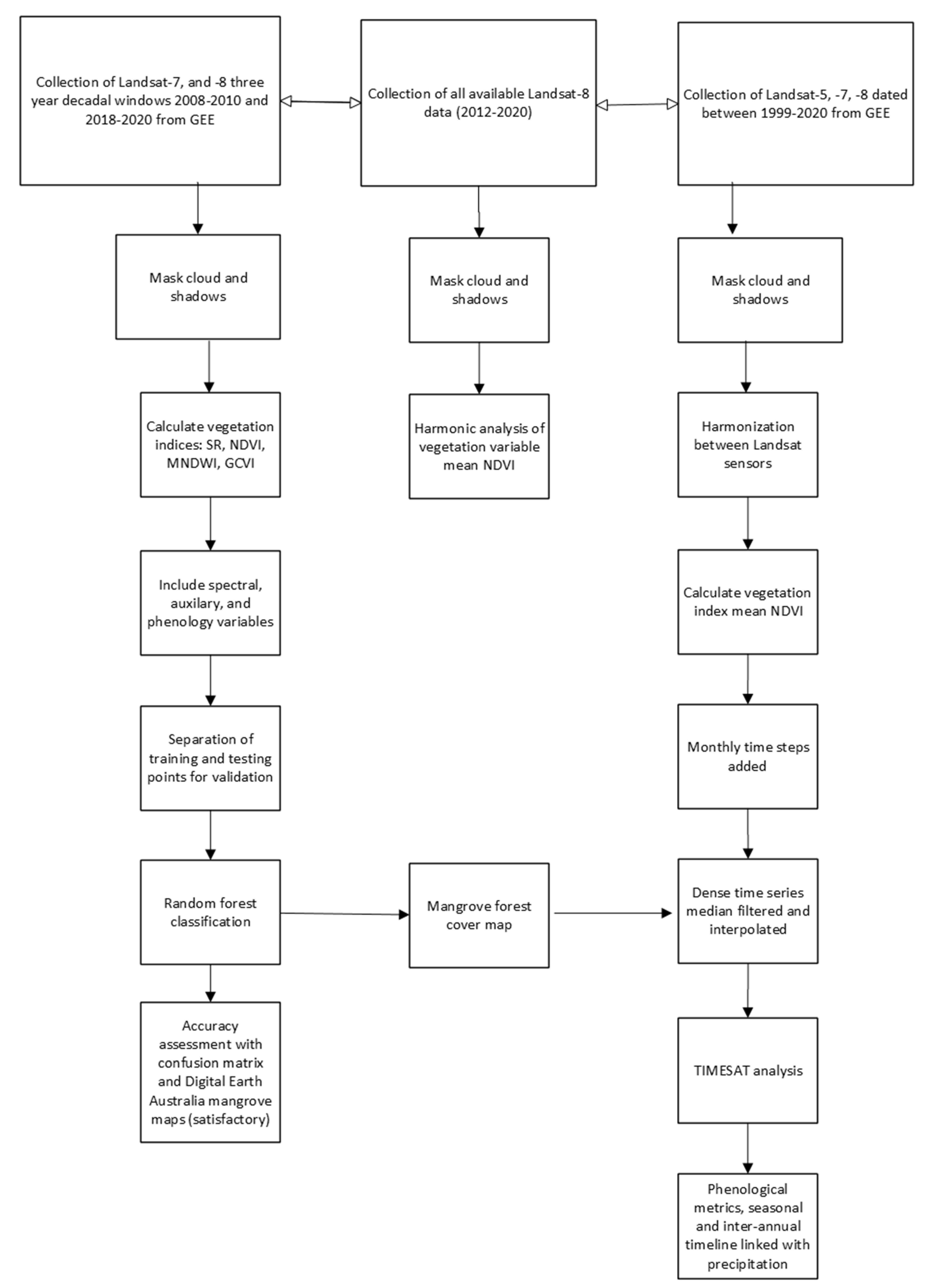
2. Materials and Methods

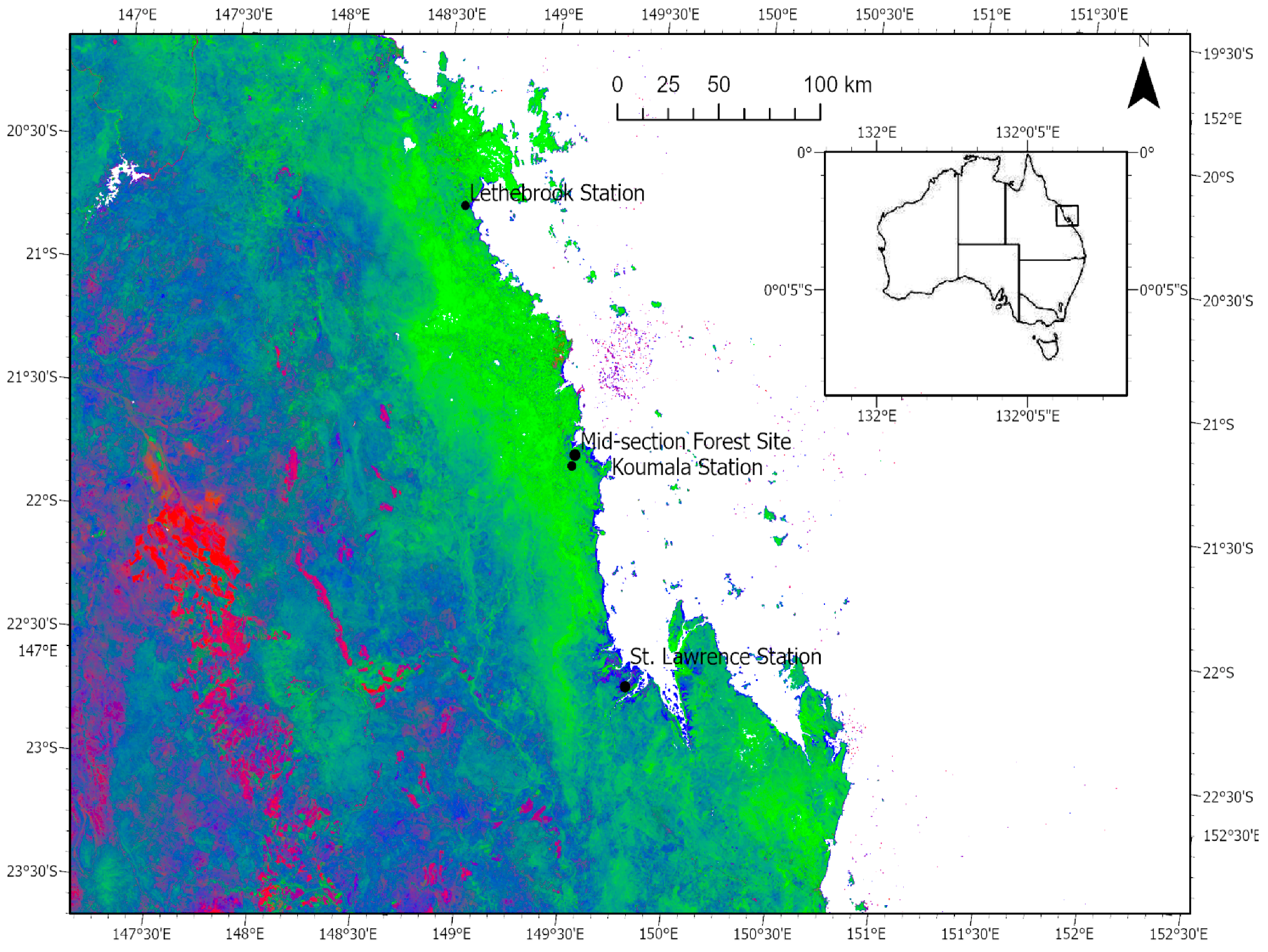
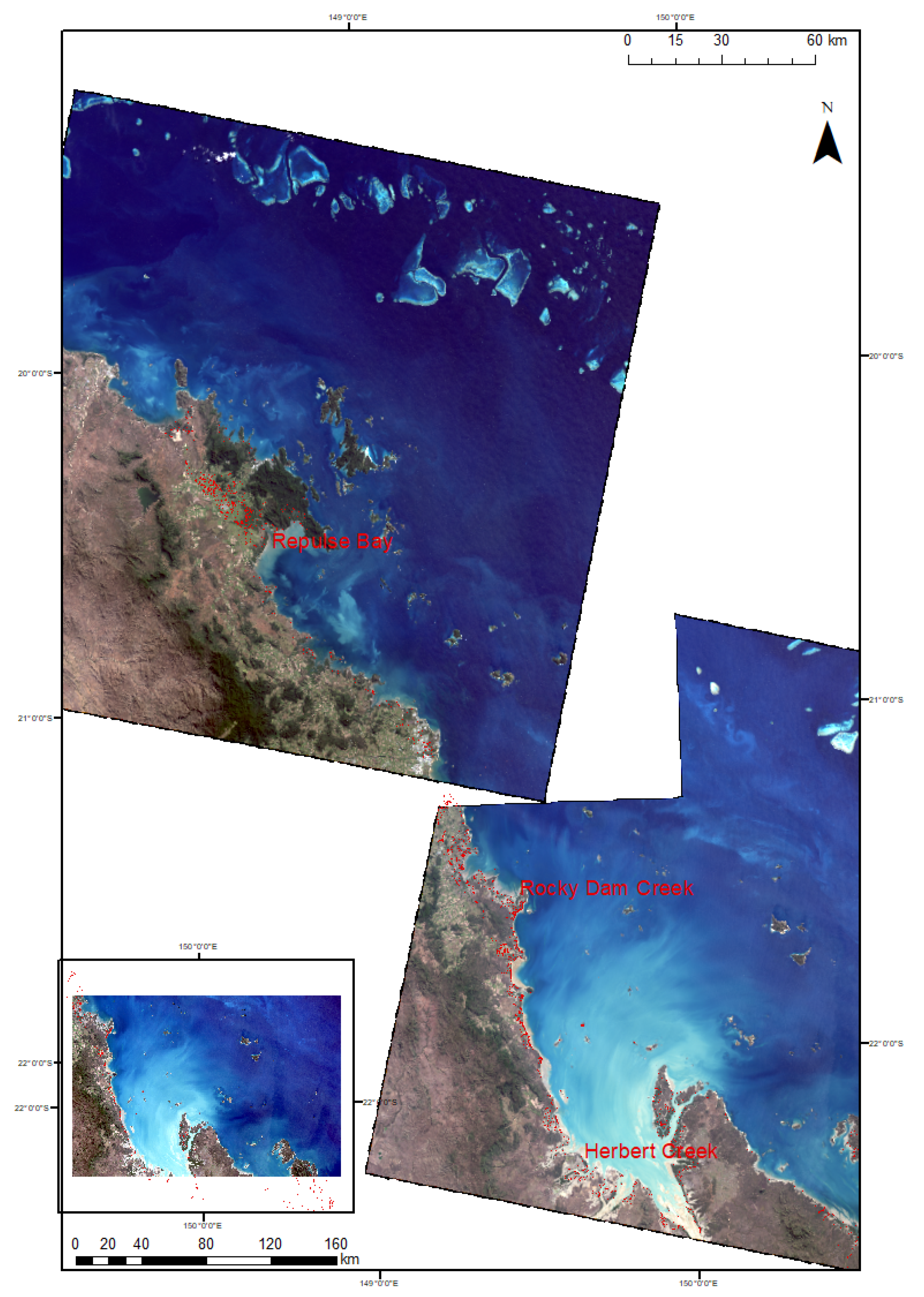
2.1. Study Area

Our study area is located within the northeast coast drainage division of the Central Queensland coast encompassing the Mackay Whitsunday Natural Resource Region and part of the Isaac Region, Central Queensland, Australia (Figure 1). Cape Palmerston National Park is positioned in the Ince Bay Receiving Waters adjacent to the World Heritage listed Great Barrier Reef. The Shoalwater and Corio Bays Area Ramsar site is located south of Cape Palmerston National Park. A large proportion of the marine waters in the Ramsar site are included in marine parks (Commonwealth and Queensland), including the Great Barrier Reef Marine Park (Commonwealth) and Great Barrier Reef Coast Marine Park (State) [41]. The Ramsar wetland supports a broad range of natural values including nationally/internationally threatened wetland species, significant species diversity and large populations of waterbirds, green turtles, dugong, and fish that use the site for vital life history functions such as roosting, nesting, feeding, and breeding. Cape Palmerston National Park is listed as a category II protected area on the International Union for Conservation of Nature (IUCN) World Database on Protected Areas and covers 7200 hectares [42]. The Shoalwater and Corio Bays Area Ramsar site covers 239,100 hectares [43].

The primary intensive land use in the region is the cultivation of sugar cane, making up 18% of the catchment area, with Mackay being the largest sugar-producing region in Australia [44]. Grazing is also an important land use, accounting for 42% [45]. The region’s estuaries directly support several commercial fisheries, e.g., East Coast Inshore Fin Fish Fishery, East Coast Otter Trawl Fishery, and Line Fishery (Reef) [46]. Additionally, recreational fishing is a considerable activity in the region, with 25% of the population participating in fishing for recreation, far greater than the state average of 15% [47]. Mangroves and associated communities cover 87,994 hectares of tidal land in the region, with nine wetland areas recognized as nationally important [48], and one Ramsar wetland recognized as internationally important. The Ramsar wetland site is subtropical with species from both temperate and tropical regions. Within the high rainfall areas of the Central Queensland coast bioregion, estuarine wetlands are about equally dominated by saltpan and samphire flats along the high intertidal area; yellow and orange mangroves (Ceriops tagal and Bruguiera spp.) dominate along the mid-intertidal area; and the stilted mangrove (Rhizophora stylosa) dominates in the lower intertidal area [48]. The river mangrove Aegicera corniculatum occupies an intermediate-upstream estuarine position while the ubiquitous grey mangrove Avicennia marina inhabits a wide range of tidal inundation levels [49]. Twenty-three tree and shrub species of mangroves are present [50]. Mean maximum temperature is between 22.7 °C in July and 30.4 °C in January, while the mean minimum temperature is between 11.4 °C in July and 23.2 °C in January. The dry season is May-November, the wet season occurs December-April. Mean annual rainfall is 1528.4 mm, while the wettest month (344.8 mm) is recorded in February. The study area is located between latitude 20°22′–22°58′S and longitude 147°19′–150°46′E (Figure 1).

2.2. Image Classification

Medium-resolution satellite imagery is suitable for mapping mangrove and wetland areas on a regional scale [52]. There are two reasons for selecting Landsat imagery: (1) it is acquired at regular intervals, and (2) it is freely available from USGS. Data processing and analysis was performed in Google Earth Engine (GEE). We used a Landsat time series to understand how mangroves have changed over time, identify areas of loss/gain and understand patterns of change in our study region. Landsat data were derived from the United States Geological Survey (USGS) Landsat 7 and 8 Collections, atmospherically corrected surface reflectance products [53]. In regions that are severely cloud-affected, such as the tropical coastal zone, it is necessary to accumulate enough Landsat data to create a cloud-free composite, therefore we chose three-year decadal windows, 2008–2010 and 2018–2020. We created a composite on a per pixel per band basis using the median reducer in GEE [27]. Topographic variables were included in the GEE image stack as a 1 arc-second (approximately 30 m) digital elevation model, the Shuttle Radar Topography Mission (SRTM), sourced from the National Aeronautics and Space Administration Agency (NASA) Jet Propulsion Lab [54]. The SRTM provides elevation and slope data subset to include only low elevation coastal areas where mangroves may be present. We masked to elevations in our study region that are less than 65 m. above mean sea level. Two distinct data sources served as reference datasets: Global Mangrove Watch (GMW) Project [55] providing the 2009 reference data; and Geoscience Australia’s Digital Earth Australia platform [56] providing the 2019 reference data. For cloud/shadow removal we filtered the Landsat composite using the quality assessment (QA) band [57] and the GEE median reducer. We calculated four VIs [58,59]: the Simple Ratio (SR) indicates healthy vegetation; the Normalized Difference Vegetation Index (NDVI), the most widely used VI and useful in understanding vegetation density and assessing changes in plant health; the Modified Normalized Difference Moisture Index (MNDWI) assesses vegetation water content; Green Chlorophyll Vegetation Index (GCVI) estimates green leaf biomass. In GEE, we applied masks to areas of low elevation and high NDVI and MNDWI. Additional masking allows us to focus on areas that are more likely to have mangroves. The auxiliary variables in the analysis were the topographic variables derived from the digital elevation model. The phenology variable was the median NDVI calculated from the time series in the three-year decadal windows, 2008–2010 and 2018–2020. The phenology variable was included to separate mangrove trees from other vegetation types (e.g., grass and crops) based on differences in seasonality [60].

Since this study seeks to evaluate predictor variables that tell us the extent of mangrove forest, only two land cover classes were generated (mangrove versus non-mangrove that includes bare soil, sand beach, water, crops, pasture, and native vegetation). We sought a supervised classification approach that is robust to normal distribution departures, can overcome limitations such as overfitting, and uses different subsets of the same training dataset [61]. Machine learning allows us to use samples of areas with and without mangroves to detect mangrove forests across a region. RF is a supervised, nonparametric, and ensemble tree-based machine learning algorithm, which has increasing use in mangrove mapping with Landsat images [62]. RF has been found to outperform comparative classification models in projection accuracy and computation cost [63,64]. Based on the predictors (Landsat bands), the trees will vote for each pixel to detect mangrove vs. non-mangrove with the most supported value assigned to each pixel. We used 100 decision trees with five predictors including the vegetation indices NDVI, MNDWI, SR, and GCVI. In GEE, the RF classifier chooses five predictors based on a random selection from seven bands in Landsat 8: ‘B5’, ‘B6’, ‘B4’, and the VIs. In the same way, the RF classifier chooses five predictors based on a random selection from seven bands in Landsat 7: ‘B4’, ‘B5’, ‘B3’, and the VIs. The training samples were collected by creating geometries of the location of mangroves using the VIs and elevation masks with Landsat false-colour composites in GEE. The total number of sample points (pixels) was 19,500. In our analysis, 80% of the sample points were randomly split and used to train the classifier. The decision trees were fully grown without pruning using a sample (with replacements) of 20% of the training data, also randomly split, to test the accuracy and validate the RF classifier [65,66]. For accuracy assessment a confusion matrix was calculated based on the sample data and classification result giving the evaluation metrics, user’s and producer’s accuracy, overall accuracy, and Kappa coefficient. Moreover, the mangrove forest maps were visually inspected and compared with high-resolution mangrove canopy cover maps from Digital Earth Australia to evaluate the performance of our method [56]. Considering that the Digital Earth Australia maps quantify the change in the extent of mangrove forest over the period 1987 to 2016 at an annual, national scale, there is concurrence with the classification maps in our study that demonstrate a regional and local approach.

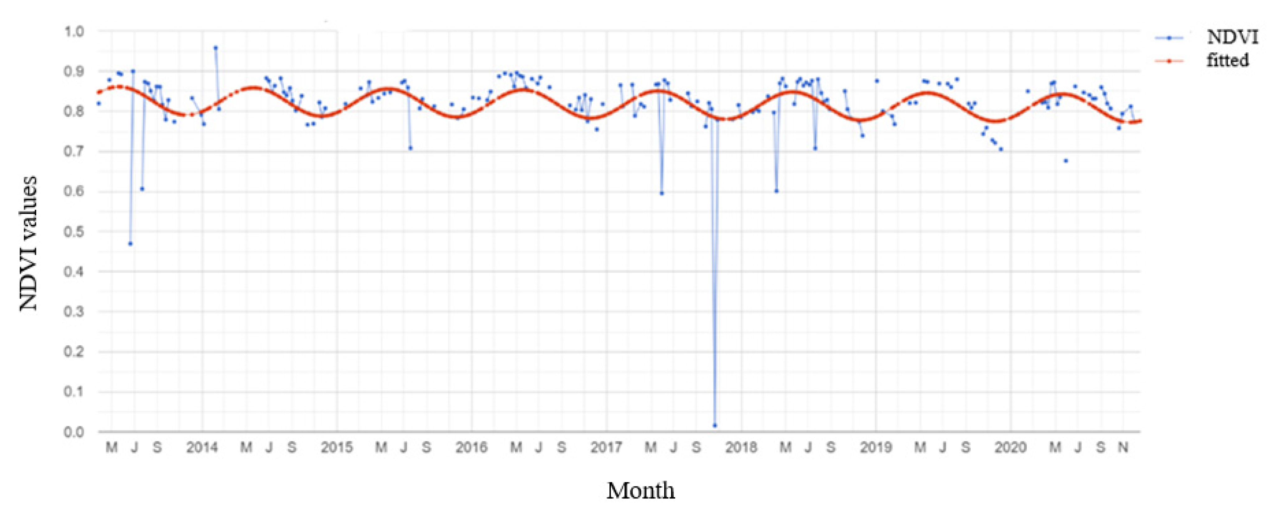
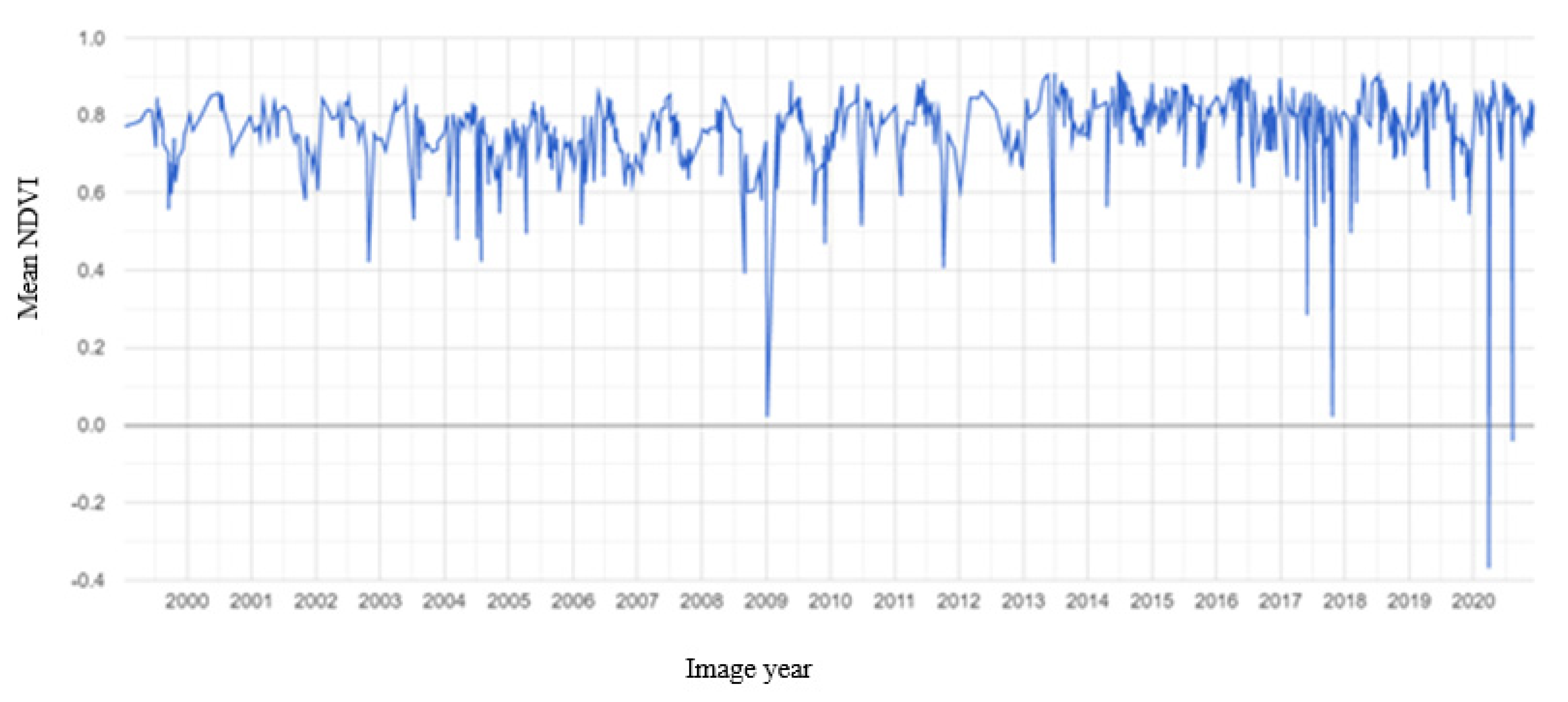
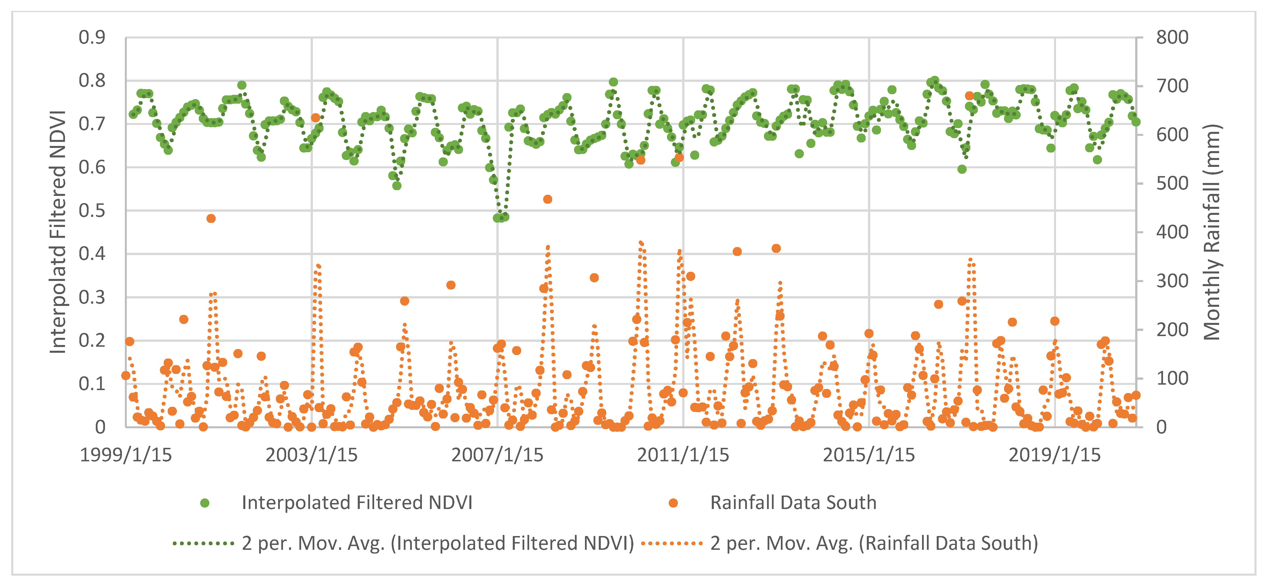
2.3. Mangrove Phenology

All available images (i.e., 2012 to 2020) for our study region (Bowen to Shoalwater and Corio Bays Area Ramsar Wetland) were acquired from the Landsat 8 surface reflectance data with a spatial resolution of 30 m and temporal resolution of 16 days and pre-processed in GEE using functions including masking clouds/cloud shadows. Images were stacked together to build a time series to be used in the models.

We used linear and harmonic regression models to analyse the seasonal parameter trends in our time series. First, we fitted an ordinary least squares model to the time series of all Landsat 8 statistical coefficients with the linear regression reducer in GEE. Second, we detrended the data to reveal underlying fluctuations in the time series. Third, we fitted Fourier-style harmonic regression equations including a trend term to each pixel and spectral component to identify phenological behaviours [37]. Harmonic regression is a mathematical technique largely focused on NDVI that is used to decompose a complex, static signal into a series of individual cosine waves (terms) and an additive term [31]. The time series is approximated as a trigonometric polynomial, with coefficients added to the harmonic model to get the amplitude (A) and phase (φ):

p_t = β₀ + β₁t +A cos(2πωt − φ) + e_t = β₀ + β₁t + β₂ cos(2πωt) + β₃ sin(2πωt) + e_t

(1)

where p_t is the value of the harmonised NDVI within a pixel obtained from the satellite data at time t, β₀ is a constant component of the regression that designates the start of greenness at each pixel, β₁ is a linear coefficient (slope/linear trend), β₂ is the cosine term coefficient, β₃ is the sine term coefficient, e_t is a random error, and ω is the angular frequency. We set ω = 1 (one cycle per unit time for an annual cycle) to fit the model to the time series.

TIMESAT Analysis

The program TIMESAT is an approach for extracting phenological parameters from remote sensing data and was partly developed from the premise that changes in vegetation phenology may be an indication of climate change [67]. The method is based on nonlinear least squares fits to the upper envelope of the NDVI data [68]. First, we applied a median filter and interpolated the missing values. Second, we used the Savitzky-Golay model and seasonal trend decomposition for a yearly growing season in tropical mangrove forests. The Savitzky-Golay filter follows within-season variations and therefore captures subtle dynamics during the growing season [69]. The result is a smoothed curve adapted to the upper envelope of the NDVI values [68]. To analyse the dense time series (1999–2020), we first created a harmonise function between L5, L7, and L8 sensors. There are small, but potentially significant differences between the spectral characteristics of Landsat ETM+ and OLI, depending on the application. It is advisable to harmonise for a long time series that spans Landsat TM, ETM+, and OLI sensors [31]. Following the harmonise function, we added the NDVI band to the collection. We extracted 13 phenological metrics for each season (21 years) from the TIMESAT program with Landsat dense time series at our study region. TIMESAT provides phenology parameters such as: start of season (SOS) depicted as initiation of a consistent upward trend in the NDVI time series, or the beginning of measurable photosynthesis in the mangrove canopy; end of season (EOS) identified as the end of consistent downward trend in the time series, or the end of measurable photosynthesis in the mangrove canopy; season length (LOS) or duration of photosynthetic activity (time of SOS to EOS); peak NDVI value (the maximum recorded NDVI value); base value (the average of the minimum values left and right of the season); amplitude (the range between the maximum NDVI and the base level or the maximum increase in canopy photosynthetic activity above the baseline); peak time (POS: time of the middle of the season, or time of maximum photosynthesis in the canopy); left derivative (rate of increase at the beginning of season or growth rate); right derivative (rate of decrease at the end of season or rate of senescence [70,71,72]. Mangrove productivity over the region was estimated using the amplitude, peak NDVI, left and right derivates, large integral, and small integral. The large integral is the function describing the season from the start to the end (an estimate of the total vegetation productivity in the annual cycle). The small integral is the difference between the function describing the season and the base level from season start to end. It is a measure of the productivity within the growing season [70,73]. Further, we used the Seasonal-Trend Decomposition by LOESS (STL) method to remove spikes and outliers in the time series and produce a smoother trendline [74].

Relationships between TIMESAT seasonality parameters were examined with linear regression models by the increasing/decreasing patterns (regression slope) and goodness-of-fit (adjusted coefficient of determination, Adjusted R²). To characterise the geographic distribution of environmental drivers of mangrove phenology, we applied climate data for 1999–2020 to the time series. Monthly rain gauge precipitation data interpolated from ground station measurements were obtained from the Australian Bureau of Meteorology online climate database (www.bom.gov.au, accessed on 1 March 2021). For the northern section of our study region, rainfall data were primarily gathered from adjacent Lethebrook Station (station number: 33041) with missing data supplemented from Bowen Station (station number: 33264). For the mid-section of our study region rainfall data were primarily gathered from the adjacent Koumala Station (station number: 33038) with missing data supplemented from Plane Creek Station (station number: 33059). For the southern section of our study region rainfall data were collected from two adjacent stations at St. Lawrence (station numbers: 33065 and 33210). As rainfall amount differs across the region, trendlines of the precipitation data were superimposed on the interpolated and filtered NDVI from the three locations across our study site: northern at Repulse Bay, mid-section at Rocky Dam Creek/Cape Palmerston National Park, and southern at Herbert Creek bordering Shoalwater and Corio Bays Area Ramsar Wetland. The peak of the season (POS) in relation to precipitation trends were compared between sites.

RF classification, linear and harmonic regression modelling and dense time series data processing was done with Google Earth Engine. The TIMESAT program was used for phenometric extraction (Figure 2). Statistical analysis was done with the R statistical environment [75] (r-project.org/).

3. Results

The aim of this research is to quantify how coastal mangrove forests have spatially and temporally changed in a decadal period (2009–2019) within estuarine catchments of the Great Barrier Reef and to explore the seasonality, climate responses, and variability of mangroves through a dense time series of satellite images in Central Queensland, Australia. Both biotic and abiotic factors constrain the phenological trajectory of a mangrove forest, e.g., regional climate, seawater and soil salinity, latitude, and local vegetation interactions, and these can vary across different locations and years. Sea surface temperatures in the Australian region have warmed by around 1 °C since 1910, with the Great Barrier Reef warming by 0.8 °C in the same period. Moreover, observations show that there has been an increase in the intensity of heavy rainfall events in Australia. (Figures S1 and S2 in the Supplementary Materials). Against the background of climate change, our study examines the phenodynamics of mangrove forests across different sites on the east coast of Australia.

3.1. Image Classification

The mangrove forest extent derived from the RF classification shows a decrease of 1480 hectares (−2.31%) over the decadal window, 2009–2019 (

Table 1. Mangrove forest extent derived from Random Forest classification with Landsat NDVI images 2009 and 2019 (Bowen to Shoalwater and Corio Bays Area Ramsar Wetland, Central Queensland).

Mangrove Extent 2009 (Ha)	Mangrove Extent 2019 (Ha)	Decrease from 2009 to 2019 (Ha)	Percent Area Decrease from 2009 to 2019 (%)
63,990	62,510	−1480	−2.31

). In ArcGIS, we generated a Landsat 8 Operational Land Imager (OLI) true-colour mosaic of our study region, overlaying the mosaic with the mangrove change map from GEE (Figure 3). The overall classification accuracy and Kappa coefficient for the 2009 and 2019 land cover maps were 95% and 95%, respectively (

Table 2. Accuracy assessment from Random Forest classification 2009 and 2019 Landsat decadal time series analysis (Bowen to Shoalwater and Corio Bays Area Ramsar Wetland, Central Queensland).

Land Class Name	Producer’s Accuracy (%)		User’s Accuracy (%)
	2009	2019	2009	2019
Mangrove forest	0.99	0.96	0.98	0.95
Non-Mangrove Forest	0.95	0.99	0.96	0.99
Overall accuracy	0.98	0.98
Kappa coefficient	0.95	0.95

). The high accuracies suggest that the RF classifier is an efficient model for projecting mangrove forest cover dynamics on both training and test datasets. The mangrove forest maps satisfactorily aligned with the high-resolution mangrove canopy cover continental-scale maps from Digital Earth Australia [56].

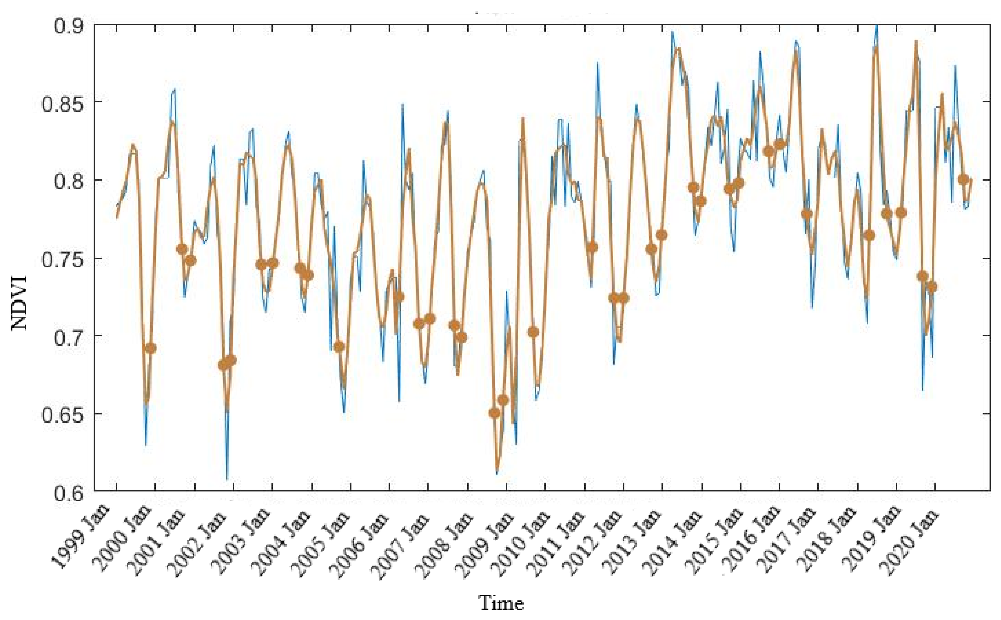
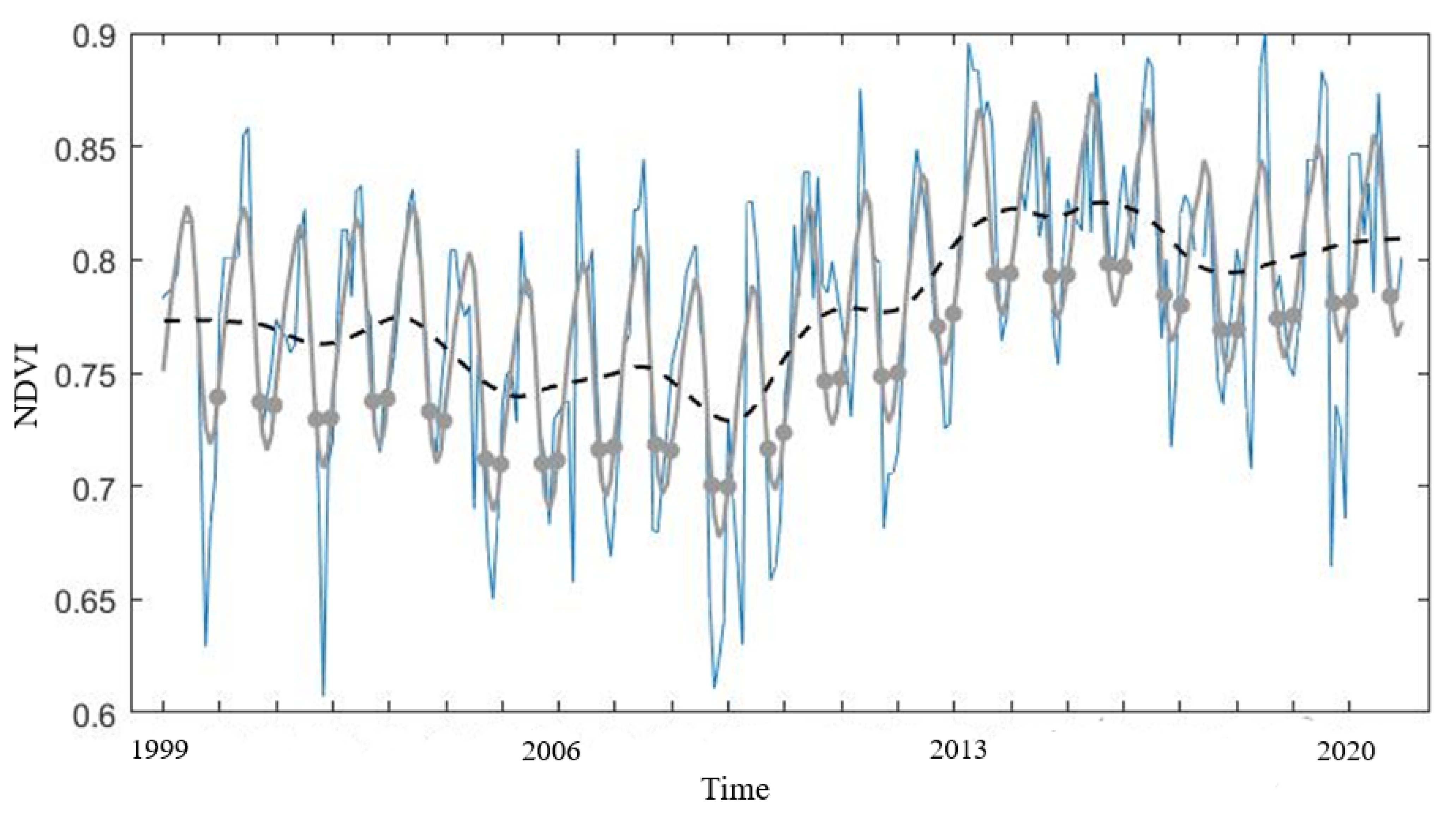
3.2. Mangrove Phenology

The detrended time series (2012–2020) shows peaks and troughs in the time series but has missing data caused by cloud masking of pixels in GEE (Figure S3 in the Supplementary Materials). Nevertheless, there is a decrease in mean NDVI across the time series with strong seasonality. Values of the peak growth and photosynthetic activity range from 0.72 to 0.9 and values of the minimum photosynthetic activity range from 0.62 to 0.82. The predicted values of the mangrove harmonic regression model were compared with the actual mean NDVI values and show a general trend in the time series (Figure 4). The seasonal trend indicates that high values were attained towards the end of the growing season (generally in winter) and low values were realized in late spring (October to November with the exception of 2018 where the lowest value was in summer, i.e., December, and 2019 where the lowest value was in early spring, i.e., September, Figure 5). We suggest that under tropical conditions, frequent cloud cover and high temperatures in spring and summer may limit the ability of mangroves to photosynthesize hence greater NDVI values occur in winter. This outcome agrees with field studies conducted by [49] with Avicennia marina in tropical Australia. We identified that tropical mangroves on the east coast of Australia display a disproportional bimodal seasonality with two periods of high mean NDVI and two periods of low NDVI values annually through the Landsat time series (1999–2020) (Figure 6 and Figure 7).

TIMESAT Analysis

In the TIMESAT program we used the Savitzky-Golay algorithm and extracted 13 attributes describing the spectro-temporal profile of mangroves for each season (

Table 3. Savitsky-Golay filter with phenometrics extracted from TIMESAT for the Landsat dense time series of mangrove forest in the mid-section of our study region, Startt.: start of season is the beginning of measurable photosynthesis in the mangrove canopy (month of the year); Endt.: end of season is the end of measurable photosynthesis in the mangrove canopy (month of the year); Length: duration of photosynthetic activity (days); Baseval.: the average of the minimum values left and right of the season (NDVI); Peakt.: time of maximum photosynthesis in the canopy (days); Peakval.: the maximum recorded NDVI value (NDVI); Ampl.: the maximum increase in canopy photosynthetic activity above the baseline (NDVI); L.deriv.: growth rate (day/NDVI); R.deriv.: rate of senescence (day/NDVI); L.integral: total productivity (day/NDVI); S.integral: seasonal productivity (day/NDVI); Startval.: value at start of season (NDVI); Endval.: value at end of season (NDVI), Bowen to Shoalwater and Corio Bays Area Ramsar Wetland, Central Queensland.

Seas.	Startt.	Endt.	Length	Baseval.	Peakt.	Peakval.	Ampl.	L.deriv.	R.deriv.	L.integral	S.integral	Startval.	Endval.
1	11.9	21.12	9.222	0.721	17.34	0.8539	0.1329	0.03167	0.03633	9.555	0.9028	0.7173	0.7779
2	26.35	33.71	7.36	0.7283	30.53	0.8131	0.08484	0.01231	0.04226	7.002	0.4479	0.7697	0.7208
3	36.6	46	9.405	0.7184	41.26	0.8337	0.1153	0.0316	0.02131	9.411	0.7901	0.7249	0.7581
4	49.65	57.38	7.728	0.7438	53.56	0.8246	0.08079	0.02252	0.02102	7.876	0.438	0.7563	0.7637
5	59.89	69.77	9.878	0.7227	63.97	0.8039	0.08119	0.01741	0.01763	9.234	0.5616	0.7596	0.7184
6	72.56	84.11	11.55	0.7069	77.04	0.7975	0.0906	0.02542	0.01493	10.56	0.6589	0.7171	0.733
7	86	94.3	8.3	0.701	90.26	0.8121	0.1111	0.02122	0.03094	8.354	0.6427	0.7359	0.7106
8	97.41	105.2	7.776	0.6941	102.1	0.8428	0.1487	0.02885	0.04959	7.722	0.7812	0.7167	0.7309
9	108.1	117.4	9.345	0.6692	113.2	0.8055	0.1363	0.02137	0.04906	8.29	0.9292	0.7234	0.6694
10	119.7	129.4	9.732	0.6548	126.1	0.8275	0.1727	0.02239	0.0459	8.826	0.9689	0.6738	0.7048
11	132.3	144	11.73	0.7202	137.4	0.8444	0.1243	0.03738	0.01137	10.41	1.043	0.7082	0.7818
12	146.9	154.2	7.284	0.7394	150.4	0.8503	0.111	0.02247	0.03217	7.939	0.5453	0.783	0.7401
13	157.4	164.9	7.516	0.7331	161.3	0.8385	0.1054	0.03491	0.02762	7.17	0.5718	0.7378	0.7706
14	169.2	178.5	9.321	0.7749	173.6	0.8965	0.1216	0.0348	0.02082	9.346	0.8217	0.7822	0.8163
15	181.6	190.5	8.946	0.8042	186.1	0.8529	0.04878	0.01479	0.01081	9.162	0.3164	0.8076	0.8202
16	193.8	201.7	7.847	0.8168	198.1	0.8744	0.05757	0.01329	0.01511	8.472	0.3035	0.8245	0.8322
17	205.6	213.2	7.618	0.8043	209.8	0.8898	0.08543	0.01478	0.03051	8.493	0.4493	0.8352	0.8076
18	215.2	224.5	9.297	0.7786	220.8	0.8359	0.05734	0.007241	0.01802	8.956	0.3909	0.7968	0.7833
19	227.8	238.2	10.41	0.7684	235	0.8755	0.1071	0.03052	0.03727	10.58	0.5864	0.7912	0.7884
20	242.6	249.4	6.795	0.7457	246.2	0.9123	0.1666	0.03448	0.05107	7.449	0.7378	0.7958	0.7623
21	251.6	261.5	9.971	0.7633	254.9	0.8783	0.115	0.03907	0.008088	9.942	0.7833	0.7555	0.817

). The filtering process preserved the trend of the original NDVI data and the fitted curve depicted the seasonal variation in forest characteristics; it, therefore, provides reliable data for the extraction of phenological information. For the mid-section of our study region (Rocky Dam Creek/Cape Palmerston National Park, Figure 3) we found the SOS to be December, EOS to be September/October, and the LOS to be 10 months. POS varied through the timeseries (February to July): 1999–2003 in June/July; 2004 in February; 2005–2006 in May; 2007–2008 in June/July; 2009–2010 in May/June; 2011–2012 in May; 2013 in April; 2014–2020 in June/July (Figure 6). There is a marked upward movement in the seasonal trend decomposition of NDVI data from the summer of 2009 to 2020 (Figure 6). Notwithstanding the length of the season gradually becoming shorter, the long integral (total productivity in the annual cycle) increased (Figure S4 in the Supplementary Materials). The trend in the peak NDVI value (maximum recorded NDVI value in the time series) increased from the summer of 2009 (Figure 7 and Figure S5 in the Supplementary Materials). In evergreen areas the small integral (productivity within the growing season) may be small even if the total vegetation production is large. The small integral and amplitude (difference between the maximal value and the base level) both declined from 2009 in our study region due to a positive change in the base value increasing the amount of green vegetation for this period (Figures S6 and S7 in the Supplementary Materials). We found a significantly high correlation (p < 0.001) between the phenology metrics from TIMESAT through the time series particularly season length and duration of the peak value (Pearson correlation coefficient r value = −0.91, Adjusted R² = 0.8182), and season (year) and season length (Pearson correlation coefficient r value = −0.91, Adjusted R² = 0.8179) indicating a dynamic trend in the cyclical behaviour of tropical mangrove forests (

Table 4. Response and explanatory variables used in the linear regression models with Pearson correlation coefficient r values and adjusted R² at significantly high values (p < 0.001).

Response Variable	Explanatory Variable Pearson Correlation Coefficient r	Adjusted R2
Season (year)	Length of season −0.91	0.818
Season (year)	Seasonal amplitude −0.78	0.597
Season (year)	Rate of senescence −0.9	0.793
Season (year)	Peak photosynthetic activity 0.7	0.462
Season (year)	Seasonal productivity −0.88	0.775
Length of season	Period of peak −0.91 photosynthetic activity	0.812
Length of season	Rate of senescence −0.9	0.721
Growth rate	Seasonal amplitude 0.87	0.755
Seasonal productivity	Rate of senescence 0.89	0.771

).

Except for the northern region, Central Queensland is largely decoupled from southern monsoonal influences and exhibits highly variable phenology that is rainfall pulse driven. Monthly rainfall was 0–800 mm at our study site, Rocky Dam Creek/Cape Palmerston National Park (Figure 3). Australia’s millennium drought of 2001–2007 is reflected in the rainfall pattern and the reduced mean NDVI trendline (Figure 8). Considerable decreases in NDVI occurred in 2001, 2002, 2004, and 2008 that are consistent with the trend of monthly rainfall. In addition to the general trend, phenological characteristics and rainfall patterns correspond with major climate events such as the EL Niño-Southern Oscillation (ENSO). The increase in precipitation from the summer of 2009 in the mid-section of our study region produced a concomitant increase in photosynthetically active growth and biomass production in mangrove forests at this site. The extreme and extended rainfall event from La Niño that occurred over Queensland in the summer of 2010/2011 was reflected in the net seasonal photosynthetic rates for this period. Further, a strong La Niño event is apparent in the Southern Oscillation Index (SOI, the difference in surface air pressure measured between Tahiti and Darwin, northern Australia) that spikes in the 2010/11 summer (Figure S8 in Supplementary Materials). In addition, a severe tropical cyclone (Tropical Cyclone Yasi, Category 5) brought an intense rainfall event in February 2011 to the entire region [76]. A relatively high rainfall pattern continued until mid-Autumn of 2017 when a severe tropical cyclone (Tropical Cyclone Debbie, Category 4) impacted the coast and destroyed coastal vegetation [77]. Recovery from the cyclone is evident in 2018 when the mean NDVI reached 0.9 at Rocky Dam Creek/Cape Palmerston National Park (Figure 8).

In comparison to the mid-section, the northern section of our study region, Repulse Bay, displays a generally higher level of mean NDVI and less temporal variability (Figure 3 and Figure S9 in the Supplementary Materials). Monthly rainfall was 0–900 mm across the time series. The POS occurred in diverse months (May to August), exemplifying a different climate pattern at this site. The northern site exhibited a NDVI decrease in 2002 similar to our mid-section site; however, the decrease occurred in the winter of 2002 (at the northern site it was early summer) and was less pronounced (Figure 9). From 2003–2020 a steady increase in NDVI activity was apparent. High rainfall peaks occurred from 2007–2012, followed by 6 years of moderate rainfall, escalating to a monsoonal trough event in January 2019, then falling to moderate rainfall conditions in 2020. A tropical cyclone (Tropical Cyclone Jasmine, Category 2) affected the northern section in February 2012. A substantial decrease in NDVI was apparent in the winter of 2017 that was not reflected in the rainfall regime but possibly occurred from the influence of cloud cover.

The southern section of our study region (Herbert Creek bordering Shoalwater and Corio Bays Area Ramsar Wetland) exhibited drier conditions than the other sections (Figure 3 and Figure S10 in the Supplementary Materials). A shorter season is apparent with POS occurring in May to July. The NDVI trendline occurred at a lower level than the other sites, but with less temporal variability. Monthly rainfall was 0–390 mm across the time series. Substantial rainfall years in 2010–2011 corresponded with the La Niño pattern of precipitation throughout Queensland but with less intensity (Figure 10). A large decrease in NDVI occurred in 2007 after prolonged low rainfall conditions. The NDVI trendline at this site reflects the El Niño year of 2006/2007 with a low rainfall level and the La Niña year of 2007/2008 with a high rainfall level. POS consistent NDVI years over the 3 sections of our study region were in 2010 with POS in May/June, 2015 with POS in June, and 2019 with POS in June/July.

4. Discussion

4.1. Change Dynamics in Mangrove Forests

With one of the richest flora in the world comprising thirty-nine species, old-world tropical mangroves found in the Indo-Pacific including Australia are notable for their attributes of species diversity, abundance, and succession and they are therefore considered to be the most dominant and important mangroves globally [78,79]. We examined decadal changes in mangrove forest cover in Great Barrier Reef catchments using a machine learning approach with the online cloud-computing platform, GEE. With GEE, we compiled a dense time series of NDVI-based Landsat imagery, inputted the time series to the TIMESAT program and investigated the phenodynamics of mangroves at different locations in our study region. This work has relevance to the maintenance of biodiversity, conservation of estuarine wetlands and mangroves, and the role of coastal forests in climate change. To our knowledge, this is the first study to examine and compare the phenology of tropical mangroves with remote sensing time series across different sites adjacent to the Great Barrier Reef, on the east coast of Australia.

We demonstrated that the mangrove extent derived from the RF classification in our study area decreased by 1480 hectares (−2.31%) over the three-year decadal window, 2009–2019. Our findings corroborate a previous study of mangrove deforestation and degradation that described a total of 11,285 hectares lost worldwide from episodic disturbance (climatic events such as dieback, disturbance mortality, climatic extremes, sea level variability) between 2000–2016 with 8004 hectares from Australia [80]. Global annual mangrove loss rates through deforestation, determined from remote sensing datasets, are estimated to be between 0.26% and 0.66% [81]. Decoupling human-induced mangrove mortality such as degradation, from declines due to episodic disturbance events is inherently difficult to achieve [82]. Moreover, spatial inconsistencies can be present as tropical coastal zones are affected by clouds and atmospheric contamination due to their proximity to oceans and the climate regime [83]. Remote sensing-based time series approaches for change detection require a series of images captured continuously throughout a time period. Thus, there is a need for substantially extra and regular image acquisitions over the area of interest [84]. As with previous studies on mangrove change dynamics [26,85,86], we found that the GEE platform provided efficient data preparation and processing capability for classification and land cover mapping with spectral, auxiliary, and phenology variables.

VIs, particularly NDVI are often used as variables in research related to regional remote sensing forest assessments and shown to be linked not only to canopy structure and leaf area index (the area of single sides leaves per area of soil) but also to canopy photosynthesis [29]. The contrast between strong near-infrared reflectance and low red reflectance of green vegetation is the basis for most VIs. NDVI, and related VIs are functional variants of the simple SR index [87]. We considered four VIs as predictor variables in our classification, SR, NDVI, MNDWI, and GCVI. VIs are commonly used in land cover classification as they increase the classification accuracy, for example: [15] selected NDVI and [88] chose SR to quantify mangrove changes over the Western Arabian Gulf and United Arab Emirates, respectively; [26] generated MNDWI for mapping mangrove extent in China. A major limitation of NDVI however, is that it saturates when mapping high amounts of biomass and cannot distinguish dense vegetation [87]. Another essential point is that NDVI is sensitive to soil, atmospheric effects, and aerosols [29,59]. Furthermore, in open mangrove canopies tidal stage can produce NDVI variations when there is no change in the vegetation amount or condition. Whereas GCVI has been developed as a proxy for chlorophyll content with Landsat surface reflectance data in crops [89], to our knowledge no previous authors have incorporated GCVI for mapping tropical forests or wetlands.

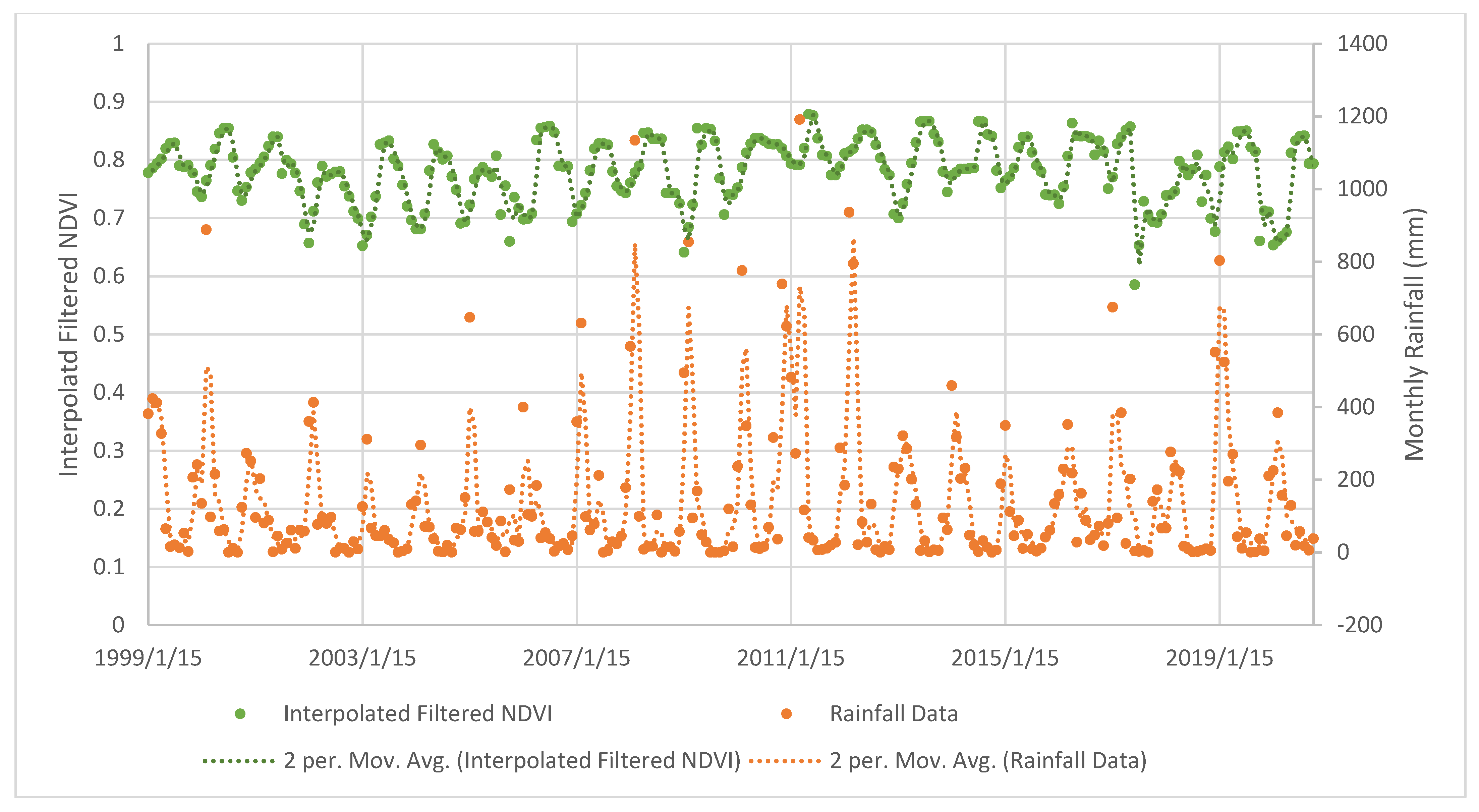
4.2. Mangrove Phenology

Our multitemporal analysis based on mean-NDVI Landsat time series (from a representative region in the study area, that is, the mid-section for approximately each month in the study period 1999–2019) revealed a strong seasonality in mangrove forests. Specifically, we found a high growth in winter and a trough of growth in late spring to summer. Such cyclical effect in seasonality has been proposed for mangroves in other tropical regions [31] and can be explained by the fact that local climate properties affect the resource availability of water through seasonal influences of tides, rainfall, and river flows and with variation in the strength of ENSO cycles [90]. Considering all available Landsat 8 imagery we demonstrated that the Fourier-style harmonic regression method provides an explicit depiction of temporal shifts in a region with substantial climate variability. Although rarely met in practice, a stringent requirement of investigating continuous intra-annual dynamics of vegetation phenology, is to acquire error-free remotely sensed data at regular time instants [91], and we successfully achieved this goal. The start, length, peak, and end of season are phenological markers that indicate the photosynthetic activity over the growing season. Specifically, we found SOS (start of the season) to be December, EOS (end of the season) to be September/October, and the LOS (length of the season) to be 10 months, regulated by the precipitation pattern in the study region. We suggest that synchronization of new leaf growth with dry season (winter) shedding, shifts canopy composition toward younger, higher radiometric green-efficient leaves, explaining obvious seasonal increases in ecosystem photosynthesis in our study region [92,93]. For instance, studies conducted on Xylocarpus spp. phenology-related litter fall in Australia demonstrate that leaf shedding occurred in the mid to late dry season on the tropical east coast [94] and Avicennia marina displayed low leafing and shedding rates throughout the year with a seasonal increase in winter [49]. The phenology of Rhizophora stylosa in both Northern and Eastern Australia was documented by [95] who detected lower photosynthetic values during the wet season and higher values during the dry season with Landsat imagery, in accordance with our study. Tropical regions experience variable climate conditions with frequent cloud cover and high temperatures during spring and summer months that may limit the capacity of mangroves to photosynthesize. Consequently, greater NDVI values occur in the winter months under cooler temperatures and more radiance. Conversely, a few studies have reported lower spectral index values during the dry season and higher values during the wet season [96,97].

The mismatch that we uncovered between the gradual contraction in the season length, and the increase in seasonal productivity can be explained by mangrove response to the resource availability of water and perhaps nutrients in tropical, coastal soils. Higher rainfall conditions as occurred from the summer of 2009 following six years of drought, produced an associated increase in photosynthetically active growth and biomass production in mangrove forests. High rainfall increases mangrove growth rates by helping to supply sediments and nutrients thereby stimulating productivity [97]. According to [98] water availability influences several ecological processes including vegetative cover, species composition, and community biomass of tidal wetlands. Freshwater is essential for mangroves to maintain the turgidity of cells and tissues, mechanisms of cell augmentation, and stomata regulation [99]. Consequently, in drought years resource-use strategies become geared towards maximum survival as opposed to rapid biomass gain.

TIMESAT Analysis

Our TIMESAT-based approach with the adaptive Savitzky-Golay filter generated smoothed data for each time step, and seasonality parameters for each identified growing season over the time series. To provide a clear and interpretable vegetation signal we chose to implement the Savitzky-Golay filter as it iteratively tightens the search window in order to capture very rapid increase or decrease in the data and follows local variations in the seasonal curve more closely [100]. Our findings that a disproportionately bimodal pattern is evident in the time series e g., late summer and winter peaks, confirm studies in phenology-based litterfall conducted on the east coast of Australia with Avicennia marina [101], which postulated that bimodality in leaf production is interrelated with position in the inter-tidal zone and frequent tidal inundation. More importantly, abiotic factors such as hydrology and photoperiod and biotic factors such as the timing of the reproductive cycle, appear to be linked to mangrove vegetative phenology [102].

The seasonal dynamics derived using TIMESAT, with mangrove NDVI time series as input, showed differences in the spatio-temporal patterns of growth dynamics. While this is the case, the three different sections of our study region are analogous in that all sections are tropical estuarine ecosystems with the same mangrove species such as the stilted mangrove Rhizophora stylosa, the grey mangrove Avicennia marina, the yellow mangrove Ceriops tagal, and the river mangrove Aegiceras corniculatum. Macroclimatic drivers such as rainfall and temperature regimes are recognized for their ability to limit and influence processes within coastal-estuarine wetlands [103]. The premise that rainfall has the greater importance in affecting biodiversity, biomass, and phenology of tropical mangrove vegetation [49] is supported by our study. For example, our observation that peaks and troughs in the NDVI trendline correspond with the trend of monthly rainfall and are magnified by climate events occurred at all three study sections, albeit with differential affects. Accordingly, we found the northern site that was also the wettest had the highest NDVI values and the southern site that was the driest had the lowest NDVI values. The site with the greatest variability in the trendline was the mid-section (Rocky Dam Creek/Cape Palmerston National Park). The mid-section was also the site with moderate monthly rainfall indicating that mangrove growth variability responds to localised patterns.

We also found that the La Niña event of 2010–2011 and its associated rainfall changes impacted vegetation growth, increasing NDVI values at all section sites. Another essential point is that the Southern Oscillation Index spikes in La Niño years, particularly 2010–2011. Indeed, a study conducted at Corio Bay in the Ramsar wetland (a generally euhaline site) in the El Niño year of 2006–2007 reported salinity reached exceedingly high values (up to 40 parts per thousand) towards the mouth. Conversely, at Corio Bay in the La Niña year of 2007–2008 salinities down to inordinately low values (23 parts per thousand) were recorded, which were associated with flooding of the adjacent Fitzoy River and local catchment run off [43]. Notably, our analysis shows that extreme climate-related salinity values such as these, are reflected in the mangrove NDVI trendline where a trough occurs in 2006–2007 followed by rise in 2007–2008 at our southern section (Herbert Creek bordering Shoalwater and Corio Bays Area Ramsar Wetland). Our results are particularly concerning for tropical mangrove forests as they highlight contemporary research on the intensification of ENSO in the coming decades with climate change [10,82].

Episodic disturbance events such as tropical cyclones and climatic extremes are purported to be responsible for approximately 80% of global mangrove loss from natural causes since 1990 [82]. In addition to coastal damage from strong winds [104], impacts from tropical cyclones include high rainfall that exacerbates the hydrological and hydrodynamic conditions [105]. Moreover, the anomalies in rainfall induce lower salinity, greater turbidity, as well as higher dissolved nutrients and phytoplankton biomass in the coastal waters when compared with typical conditions [106]. The frequency and intensity of cyclones and storms has increased as a consequence of greater sea-surface temperature, with further escalation predicted under most climate change scenarios [107,108]. Greater cyclone frequency has compounding effects on mangrove forests and may extend or halt mangrove recovery [107]. Our findings show decreases in the NDVI values associated with the occurrence of tropical cyclones in each section of our study region. Tropical Cyclone Yasi impacted all three sites in 2011, Tropical Cyclone Jasmine destroyed the northern section site in 2012, and Tropical Cyclone Debbie devastated the mid-section and southern section sites in 2017, which was the highest precipitation event over the time series.

4.3. Limitations of the Study

Remote sensing data and tools are fundamental methods for measuring land cover, but there are key drawbacks in the change detection of wetlands such as mangrove forests. The need for assessing accuracy of a map generated from any remotely sensed product has become a universal requirement and an integral part of any classification project. The user community needs to know the accuracy of the classified image data being presented [109] otherwise the classification lacks robust validation which could have serious implications for some users and may lessen their confidence in remote sensing as a source of land cover data. Accuracy assessment (1) allows self-evaluation and to learn from mistakes in the classification process; (2) provides quantitative comparison of the classified maps; (3) ensures greater reliability of the resulting maps/spatial information. Therefore, we presented robust validation methods that detail the user’s and producer’s accuracies of change with Kappa coefficient. Furthermore, we compared the mangrove forest classified maps with Digital Earth Australia high-resolution imagery (at the continental-scale) for visual refinement and to evaluate the performance of our method [56]. The second key drawback is that there can be a similarity of spectral reflectance in the NIR and SWIR regions between mangrove forest and the mixture of other natural vegetation and water at high tide compared to that obtained at low tide [26,86,110]. The third drawback is that quantification is difficult in long-term studies because inconsistencies and gaps in data collection due to observation error are common [111]. The fourth drawback is that temperate climates use simple spring indicators and measures related to 1 January that are not appropriate for tropical phenology because of the circularity of the data. Thus, tropical phenological approaches necessitate taking account of data circularity, be flexible, quantitative, and attribute confidence to conclusions [112]. Finally, a key drawback is that in similar climate conditions, genotypes of mangrove species spread across a study region may vary enough to exemplify different phenophases. In addition, although mangroves are highly specialized and occupy unique and heterogeneous suites of habitats within Australia, they are not a genetic entity but an ecological one [98,112,113]. Consequently, our study has accessed nearby weather stations to our section sites such that localised and subtle climate variations (known to influence phenophases) in location are recorded, and this has reflected in the timeline signals.

4.4. Implications for the Conservation of Mangrove Forests

Growing evidence of mangrove’s ability to sequester and store carbon has brought attention to their conservation value from international climate change policy and decision makers [114]. Although estuarine monitoring is almost completely absent at Shoalwater and Corio Bay Areas Ramsar Wetland, it is critical to establish a monitoring program to provide baseline assessments of vegetation seasonality in relation to weather patterns and detect responses to extreme events. The Ramsar Convention on Wetlands is an intergovernmental treaty with Parties to the Convention from 171 countries. The purpose of the Ramsar Convention is to promote wetland conservation and wise use to ensure that the benefits of wetlands contribute towards meeting the UN Sustainable Development goals, Aichi Biodiversity Targets, Paris Agreement on Climate Change, and other related international commitments [115]. The United Nations’ 2030 Agenda for Sustainable Development together with SDGs require the monitoring and mapping of mangroves through the sustainable development indicator 6.6.1: “change in the extent of water-related ecosystems over time” [11]. Monitoring of mangrove forests is critical to preserve the ecosystem services they provide such as pollution control, detoxification, and regulation of natural hazards. Hydrologic conditions, land use, and management are important drivers of coastal vegetation communities with many land use changes developing over decades. So far, studies on tropical forests and mangrove cover with phenodynamics have been limited by the unavailability of suitable remote sensing imagery. Dense time series of satellite images has allowed a comprehensive understanding of mangrove phenology and its relation to climate factors across different sites. Our results are of relevance for conservation strategies of tropical coastal wetlands in Australia that account for foundation species and their seasonal responses to climate drivers.

5. Conclusions

In this paper, we demonstrated an operational method to (1) map mangrove forests in Central Queensland, Australia using an NDVI time series, which was built in GEE from Landsat imagery, and (2) examine seasonal and inter-annual changes in mangrove phenology extracted with the TIMESAT program, and linked to natural and extreme climate variability. Surprisingly, estuarine monitoring has been absent in the coastal ecosystems of Shoalwater and Corio Bay Ramsar Wetland. Mangrove forests in this southern section of our study region are bounded by an internationally recognized Ramsar Wetland Treaty and therefore changes in their ecology are important for Australia’s reporting commitments to the Ramsar Convention. Policy guidelines of the Convention underline that urgent action is needed to raise awareness of the benefits of wetlands, with greater safeguards for their survival. We propose that a regulated monitoring program be instigated so that information can be gathered on the change dynamics and seasonality of estuarine communities and mangroves under threat from episodic disturbances.

Monitoring is essential, ideally before and particularly after an extreme event, to improve our knowledge of the connections among climate, weather, and biodiversity. Our objective to acquire long-term and spatially extensive data was due to the highly variable nature of biological data, and the need to examine periodical events at different locations. The detection of responses to extreme events is important to improve understanding of the connections between climate, extreme weather events, and biodiversity. Such knowledge is essential to inform conservation management attempts to mitigate the impacts of extreme events with ongoing climate change.

References

1. Lee, S.Y.; Primavera, J.H.; Dahdouh-Guebas, F.; McKee, K.; Bosire, J.O.; Cannicci, S.; Diele, K.; Fromard, F.; Koedam, N.; Marchand, C.; et al. Ecological role and services of tropical mangrove ecosystems: A reassessment. Glob. Ecol. Biogeogr. 2014, 23, 726–743. [Google Scholar] [CrossRef]
2. Sheaves, M.; Johnston, R.; Baker, R. Use of mangroves by fish: New insights from in-forest videos. Mar. Ecol. Prog. Ser. 2016, 549, 167–182. [Google Scholar] [CrossRef] [Green Version]
3. Macreadie, P.I.; Anton, A.; Raven, J.A.; Beaumont, N.; Connolly, R.M.; Friess, D.A.; Kelleway, J.J.; Kennedy, H.; Kuwae, T.; Lavery, P.S.; et al. The future of Blue Carbon science. Nat. Commun. 2019, 10, 3998. [Google Scholar] [CrossRef] [PubMed] [Green Version]
4. Adame, M.F.; Connolly, R.M.; Turschwell, M.P.; Lovelock, C.E.; Fatoyinbo, T.; Lagomasino, D.; Goldberg, L.A.; Holdorf, J.; Friess, D.A.; Sasmito, S.D.; et al. Future carbon emissions from global mangrove forest loss. Glob. Chang. Biol. 2021. [Google Scholar] [CrossRef]
5. The International Council on Clean Transportation. Vision 2050: A Strategy to Decarbonize the Global Transport Sector by Mid-Century; The International Council on Clean Transportation: Washington, DC, USA, 2020; pp. 1–25. [Google Scholar]
6. Friess, D.A.; Yando, E.S.; Abuchahla, G.M.O.; Adams, J.B.; Cannicci, S.; Canty, S.W.J.; Cavanaugh, K.C.; Connolly, R.M.; Cormier, N.; Dahdouh-Guebas, F.; et al. Mangroves give cause for conservation optimism, for now. Curr. Biol. 2020, 30, R153–R154. [Google Scholar] [CrossRef] [PubMed] [Green Version]
7. Saintilan, N.; Rogers, K.; Kelleway, J.J.; Ens, E.; Sloane, D.R. Climate change impacts on the coastal wetlands of Australia. Wetlands 2018, 38, 1145–1154. [Google Scholar] [CrossRef]
8. Spalding, M.D.; Ruffo, S.; Lacambra, C.; Meliane, I.; Hale, L.Z.; Shepard, C.C.; Beck, M.W. The role of ecosystems in coastal protection: Adapting to climate change and coastal hazards. Ocean Coast. Manag. 2014, 90, 50–57. [Google Scholar] [CrossRef]
9. Fang, X.; Hou, X.; Li, X.; Hou, W.; Nakaoka, M.; Yu, X. Ecological connectivity between land and sea: A review. Ecol. Res. 2018, 33, 51–61. [Google Scholar] [CrossRef]
10. Lovelock, C.E.; Feller, I.C.; Reef, R.; Hickey, S.; Ball, M.C. Mangrove dieback during fluctuating sea levels. Sci. Rep. 2017, 7, 1680. [Google Scholar] [CrossRef]
11. UNGA: United Nations General Assembly. Work of the Statistical Commission Pertaining to the 2030 Agenda for Sustainable Development: Resolution/Adopted by the General Assembly (A/RES/71/313); UNGA: New York, NY, USA, 2017. [Google Scholar]
12. de Beurs, K.M.; Henebry, G.M. Spatio-temporal statistical methods for modelling land surface phenology. In Phenological Research: Methods for Environmental and Climate Change Analysis; Hudson, I.L., Keatley, M.R., Eds.; Springer: New York, NY, USA, 2010; pp. 177–208. [Google Scholar]
13. Hostert, P.; Griffiths, P.; van der Linden, S.; Pflugmacher, D. Time series analyses in a new era of optical satellite data. In Remote Sensing Time Series; Springer International Publishing: Cham, Switzerland, 2015; pp. 25–41. [Google Scholar] [CrossRef]
14. Keenan, R.J. Climate change impacts and adaptation in forest management: A review. Ann. For. Sci. 2015, 72, 145–167. [Google Scholar] [CrossRef] [Green Version]
15. Li, W.; El-Askary, H.; Qurban, M.A.; Li, J.; ManiKandan, K.P.; Piechota, T. Using multi-indices approach to quantify mangrove changes over the Western Arabian Gulf along Saudi Arabia coast. Ecol. Indic. 2019, 102, 734–745. [Google Scholar] [CrossRef]
16. Wu, N.; Shi, R.; Zhuo, W.; Zhang, C.; Zhou, B.; Xia, Z.; Tao, Z.; Gao, W.; Tian, B. A classification of tidal flat wetland vegetation combining phenological features with Google Earth Engine. Remote Sens. 2021, 13, 443. [Google Scholar] [CrossRef]
17. Keatley, M.R.; Hudson, I.L. Introduction and overview. In Phenological Research: Methods for Environmental and Climate Change Analysis; Hudson, I.L., Keatley, M.R., Eds.; Springer: New York, NY, USA, 2010; pp. 1–22. [Google Scholar] [CrossRef]
18. Younes, N.; Joyce, K.E.; Maier, S.W. All models of satellite-derived phenology are wrong, but some are useful: A case study from northern Australia. Int. J. Appl. Earth Obs. Geoinf. 2021, 97, 102285. [Google Scholar] [CrossRef]
19. Jimenez Galo, A.J. Monitoring of tropical forest cover with remote sensing. In Tropical Forestry Handbook; Pancel, L., Köhl, M., Eds.; Springer: Berlin, Germany, 2016; pp. 1–19. [Google Scholar] [CrossRef]
20. DeVries, B.; Pratihast, A.K.; Verbesselt, J.; Kooistra, L.; Herold, M. Characterizing forest change using community-based monitoring data and Landsat time series. PLoS ONE 2016, 11, e0147121. [Google Scholar] [CrossRef] [PubMed]
21. Duarte, E.; Barrera, J.A.; Dube, F.; Casco, F.; Hernández, A.J.; Zagal, E. Monitoring approach for tropical coniferous forest degradation using remote sensing and field data. Remote Sens. 2020, 12, 2531. [Google Scholar] [CrossRef]
22. Souza, C.M.; Shimbo, J.Z.; Rosa, M.R.; Parente, L.L.; Alencar, A.A.; Rudorff, B.F.T.; Hasenack, H.; Matsumoto, M.; Ferreira, G.L.; Souza-Filho, P.W.M.; et al. Reconstructing three decades of land use and land cover changes in Brazilian biomes with Landsat archive and Earth Engine. Remote Sens. 2020, 12, 2735. [Google Scholar] [CrossRef]
23. Criminisi, A. Decision Forests: A unified framework for classification, regression, density estimation, manifold learning and semi-supervised learning. Found. Trends Comput. Graph. Vis. 2011, 7, 81–227. [Google Scholar] [CrossRef]
24. Hastie, T.; Tibshirani, R.; Friedman, J. The Elements of Statistical Learning: Data Mining, Inference, and Prediction, 2nd ed.; Springer: New York, NY, USA, 2017. [Google Scholar]
25. Pham, L.T.H.; Brabyn, L. Monitoring mangrove biomass change in Vietnam using SPOT images and an object-based approach combined with machine learning algorithms. ISPRS J. Photogramm. Remote Sens. 2017, 128, 86–97. [Google Scholar] [CrossRef]
26. Hu, L.; Li, W.; Xu, B. Monitoring mangrove forest change in China from 1990 to 2015 using Landsat-derived spectral-temporal variability metrics. Int. J. Appl. Earth Obs. Geoinf. 2018, 73, 88–98. [Google Scholar] [CrossRef]
27. Diniz, C.; Cortinhas, L.; Nerino, G.; Rodrigues, J.; Sadeck, L.; Adami, M.; Souza-Filho, P. Brazilian mangrove status: Three decades of satellite data analysis. Remote Sens. 2019, 11, 808. [Google Scholar] [CrossRef] [Green Version]
28. Bihamta Toosi, N.; Soffianian, A.R.; Fakheran, S.; Pourmanafi, S.; Ginzler, C.; Waser, T.L. Land cover classification in mangrove ecosystems based on VHR satellite data and machine learning—an upscaling approach. Remote Sens. 2020, 12, 2884. [Google Scholar] [CrossRef]
29. Xue, J.; Su, B. Significant remote sensing vegetation indices: A review of developments and applications. J. Sens. 2017, 2017, 1353691. [Google Scholar] [CrossRef] [Green Version]
30. Grace, J.; Nichol, C.; Disney, M.; Lewis, P.; Quaife, T.; Bowyer, P. Can we measure terrestrial photosynthesis from space directly, using spectral reflectance and fluorescence? Glob. Chang. Biol. 2007, 13, 1484–1497. [Google Scholar] [CrossRef]
31. Venkatappa, M.; Sasaki, N.; Shrestha, R.P.; Tripathi, N.K.; Ma, H.O. Determination of vegetation thresholds for assessing land use and land use changes in Cambodia using the Google Earth Engine cloud-computing platform. Remote Sens. 2019, 11, 1514. [Google Scholar] [CrossRef] [Green Version]
32. Xiao, X.; Zhang, J.; Yan, H.; Wu, W.; Biradar, C. Land surface phenology. In Phenology of Ecosystem Processes: Applications in Global Change Research; Noormets, A., Ed.; Springer: New York, NY, USA, 2009; pp. 247–270. [Google Scholar] [CrossRef]
33. Priyadarshi, N.; Chowdary, V.M.; Srivastava, Y.K.; Das, I.C.; Jha, C.S. Reconstruction of time series MODIS EVI data using de-noising algorithms. Geocarto Int. 2018, 33, 1095–1113. [Google Scholar] [CrossRef]
34. Shamim Hasan Mandal, M.; Kamruzzaman, M.; Hosaka, T. Elucidating the phenology of the Sundarbans mangrove forest using 18-year time series of MODIS vegetation indices. Tropics 2020, 29, 41–55. [Google Scholar] [CrossRef]
35. Sadinski, W.; Gallant, A.L.; Roth, M.; Brown, J.; Senay, G.; Brininger, W.; Jones, P.M.; Stoker, J. Multi-year data from satellite- and ground-based sensors show details and scale matter in assessing climate’s effects on wetland surface water, amphibians, and landscape conditions. PLoS ONE 2018, 13, e0201951. [Google Scholar] [CrossRef]
36. Kelly, N. Accounting for correlated error structure within phenological data: A case study of trend analysis of snowdrop flowering. In Phenological Research: Methods for Environmental and Climate Change Analysis; Hudson, L.L., Keatley, M.R., Eds.; Springer: New York, NY, USA, 2010; pp. 271–298. [Google Scholar] [CrossRef]
37. Adams, B.; Iverson, L.; Matthews, S.; Peters, M.; Prasad, A.; Hix, D.M. Mapping forest composition with Landsat time series: An evaluation of seasonal composites and harmonic regression. Remote Sens. 2020, 12, 610. [Google Scholar] [CrossRef] [Green Version]
38. Li, D.; Lu, D.; Wu, M.; Shao, X.; Wei, J. Examining land cover and greenness dynamics in Hangzhou Bay in 1985–2016 using Landsat time-series data. Remote Sens. 2017, 10, 32. [Google Scholar] [CrossRef] [Green Version]
39. Lamb, B.T.; Tzortziou, M.A.; McDonald, K.C. Evaluation of approaches for mapping tidal wetlands of the Chesapeake and Delaware Bays. Remote Sens. 2019, 11, 366. [Google Scholar] [CrossRef] [Green Version]
40. Campbell, A.D.; Wang, Y. Salt marsh monitoring along the mid-Atlantic coast by Google Earth Engine enabled time series. PLoS ONE 2020, 15, e0229605. [Google Scholar] [CrossRef] [Green Version]
41. Department of Agriculture Water and the Environment. Directory of Important Wetlands in Australia-Information Sheet, Sarina Inlet-Ince Bay Aggregation-QLD053. Available online: https://www.environment.gov.au/cgi-bin/wetlands/report.pl (accessed on 1 March 2021).
42. Chamberlain, D.; Phinn, S.; Possingham, H. Remote sensing of mangroves and estuarine communities in Central Queensland, Australia. Remote Sens. 2020, 12, 197. [Google Scholar] [CrossRef] [Green Version]
43. Ronan, M. Ramsar Information Sheet: Shoalwater and Corio Bays Area, Australia; Queensland Department of Environment and Heritage Protection: Brisbane, QLD, Australia, 2018.
44. Folkers, A.; Rohde, K.; Delaney, K.; Flett, I. Mackay Whitsunday Water Quality Improvement Plan 2014–2021; Reef Catchments: Mackay, QLD, Australia, 2014. [Google Scholar]
45. Reef Catchments Limited. Natural Resource Management Plan; Mackay Whitsunday Isaac: Mackay, QLD, Australia, 2014. [Google Scholar]
46. Pascoe, S.; Innes, J.; Tobin, R.; Stoeckle, N.; Paredes, S.; Dauth, K. Beyond GVP: The Value of Inshore Commercial Fisheries to Fishers and Consumers in Regional Communities on Queensland’s East Coast; FRDC Project No 2013-301: Deakin, VIC, Australia, 2016. [Google Scholar]
47. Webley, J.; McInnes, K.; Teixeira, D.; Lawson, A.; Quinn, R. Statewide Recreational Fishing Survey 2013-14; Department of Agriculture and Fisheries: Brisbane, QLD, Australia, 2015. [Google Scholar]
48. Reef Catchments. State of the Region Report; Mackay Whitsunday Isaac: Mackay, QLD, Australia, 2013. [Google Scholar]
49. Duke, N.C. Australia’s Mangroves: The Authoritative Guide to Australia’s Mangrove Plants; University of Queensland: Brisbane, QLD, Australia, 2006. [Google Scholar]
50. Duke, N.C.; Larkum, A.W.D. Mangroves and seagrasses. In The Great Barrier Reef: Biology, environment and Management, 2nd ed.; Hutchings, P., Kingsford, M., Hoegh-Guldberg, O., Eds.; CSIRO: Clayton South, VIC, Australia, 2019; pp. 219–228. [Google Scholar]
51. AusCover. Seasonal Fractional Vegetation Cover for Queensland Derived from USGS Landsat Images. Available online: http://data.auscover.org.au/xwiki/bin/view/Product+pages/Landsat+Seasonal+Fractional+Cover (accessed on 1 March 2021).
52. Kuenzer, C.; Bluemel, A.; Gebhardt, S.; Quoc, T.V.; Dech, S. Remote sensing of mangrove ecosystems: A review. Remote Sens. 2011, 3, 878–928. [Google Scholar] [CrossRef] [Green Version]
53. Vermote, E.; Justice, C.; Claverie, M.; Franch, B. Preliminary analysis of the performance of the Landsat 8/OLI land surface reflectance product. Remote Sens. Environ. 2016, 185, 46–56. [Google Scholar] [CrossRef]
54. Farr, T.G.; Rosen, P.A.; Caro, E.; Crippen, R.; Duren, R.; Hensley, S.; Kobrick, M.; Paller, M.; Rodriguez, E.; Roth, L.; et al. The Shuttle Radar Topography Mission. Rev. Geophys. 2007, 45, 1–33. [Google Scholar] [CrossRef] [Green Version]
55. Bunting, P.; Rosenqvist, A.; Lucas, R.; Rebelo, L.-M.; Hilarides, L.; Thomas, N.; Hardy, A.; Itoh, T.; Shimada, M.; Finlayson, M. The global mangrove watch-a new 2010 global baseline of mangrove extent. Remote Sens. 2018, 10, 1669. [Google Scholar] [CrossRef] [Green Version]
56. Lymburner, L.; Bunting, P.; Lucas, R.; Scarth, P.; Alam, I.; Phillips, C.; Ticehurst, C.; Held, A. Mapping the multi-decadal mangrove dynamics of the Australian coastline. Remote Sens. Environ. 2020, 238, 111185. [Google Scholar] [CrossRef]
57. USGS. Landsat Collection 1 Level 1 Product Definition; United States Geological Survey: Vermillion, SD, USA, 2017; pp. 1–24.
58. Wu, C.; Niu, Z.; Gao, S. The potential of the satellite derived green chlorophyll index for estimating midday light use efficiency in maize, coniferous forest and grassland. Ecol. Indic. 2012, 14, 66–73. [Google Scholar] [CrossRef]
59. Pastor-Guzman, J.; Atkinson, P.; Dash, J.; Rioja-Nieto, R. Spatiotemporal variation in mangrove chlorophyll concentration using Landsat 8. Remote Sens. 2015, 7, 14530–14558. [Google Scholar] [CrossRef] [Green Version]
60. Karlson, M.; Ostwald, M.; Reese, H.; Sanou, J.; Tankoano, B.; Mattsson, E. Mapping tree canopy cover and aboveground biomass in Sudano-Sahelian Woodlands using Landsat 8 and Random Forest. Remote Sens. 2015, 7, 10017–10041. [Google Scholar] [CrossRef] [Green Version]
61. Berhane, T.M.; Lane, C.R.; Wu, Q.; Autrey, B.C.; Anenkhonov, O.A.; Chepinoga, V.V.; Liu, H. Decision-Tree, rule-based, and Random Forest classification of high-resolution multispectral imagery for wetland mapping and inventory. Remote Sens. 2018, 10, 580. [Google Scholar] [CrossRef] [Green Version]
62. Pham, T.D.; Xia, J.; Ha, N.T.; Bui, D.T.; Le, N.N.; Tekeuchi, W. A review of remote sensing approaches for monitoring blue carbon ecosystems: Mangroves, seagrasses and salt marshes during 2010-2018. Sensors 2019, 19, 1933. [Google Scholar] [CrossRef] [Green Version]
63. Belgiu, M.; Drăguţ, L. Random forest in remote sensing: A review of applications and future directions. ISPRS J. Photogramm. Remote Sens. 2016, 114, 24–31. [Google Scholar] [CrossRef]
64. Liu, B.; Gao, L.; Li, B.; Marcos-Martinez, R.; Bryan, B.A. Nonparametric machine learning for mapping forest cover and exploring influential factors. Landsc. Ecol. 2020, 35, 1683–1699. [Google Scholar] [CrossRef]
65. Pelletier, C.; Valero, S.; Inglada, J.; Champion, N.; Dedieu, G. Assessing the robustness of Random Forests to map land cover with high resolution satellite image time series over large areas. Remote Sens. Environ. 2016, 187, 156–168. [Google Scholar] [CrossRef]
66. Maxwell, A.E.; Warner, T.A.; Fang, F. Implementation of machine-learning classification in remote sensing: An applied review. Int. J. Remote Sens. 2018, 39, 2784–2817. [Google Scholar] [CrossRef] [Green Version]
67. Eklundh, L.; Jonsson, P. TIMESAT for processing time-series data from satellite sensors for land surface monitoring. In Multitemporal Remote Sensing: Methods and Applications; Ban, Y., Ed.; Springer International Publishing: Cham, Switzerland, 2016; Volume 20, pp. 177–194. [Google Scholar]
68. Jönsson, P.; Eklundh, L. TIMESAT—A program for analyzing time-series of satellite sensor data. Comput. Geosci. 2004, 30, 833–845. [Google Scholar] [CrossRef] [Green Version]
69. Stanimirova, R.; Cai, Z.; Melaas, E.K.; Gray, J.M.; Eklundh, L.; Jönsson, P.; Friedl, M.A. An empirical assessment of the MODIS land cover dynamics and TIMESAT land surface phenology algorithms. Remote Sens. 2019, 11, 2201. [Google Scholar] [CrossRef] [Green Version]
70. Valderrama-Landeros, L.; España-Boquera, M.L.; Baret, F.; Sánchez-Vargas, N.; Sáenz-Romero, C. Capacity of phenological data derived from Cyclopes Lai for the year 2000 to distinguish land cover types in the State of MichoacÁn, Mexico. Revista Chapingo Serie Ciencias Forestales Y Del Ambiente 2014, 20, 261–276. [Google Scholar] [CrossRef] [Green Version]
71. Hentze, K.; Thonfeld, F.; Menz, G. Evaluating crop area mapping from MODIS time-series as an assessment tool for Zimbabwe’s “Fast Track Land Reform Programme”. PLoS ONE 2016, 11, e0156630. [Google Scholar] [CrossRef]
72. Kong, F.; Li, X.; Wang, H.; Xie, D.; Li, X.; Bai, Y. Land cover classification based on fused data from GF-1 and MODIS NDVI time series. Remote Sens. 2016, 8, 741. [Google Scholar] [CrossRef] [Green Version]
73. Davis, C.L.; Hoffman, M.T.; Roberts, W. Long-term trends in vegetation phenology and productivity over Namaqualand using the GIMMS AVHRR NDVI3g data from 1982 to 2011. S. Afr. J. Bot. 2017, 111, 76–85. [Google Scholar] [CrossRef]
74. Ghosh, S.; Mishra, D. Analyzing the long-term phenological trends of salt marsh ecosystem across Coastal Louisiana. Remote Sens. 2017, 9, 1340. [Google Scholar] [CrossRef] [Green Version]
75. R Core Team. R: A Language and Environment for Statistical Computing. 2020. Available online: https://www.R-project.org/ (accessed on 1 March 2021).
76. Bureau of Meteorology. Tropical Cyclone Reports. Available online: http://www.bom.gov.au/cyclone/tropical-cyclone-knowledge-centre/history/past-tropical-cyclones/ (accessed on 1 March 2021).
77. Commonwealth of Australia. Reef 2050 Long Term Sustainability Plan 2018; Commonwealth of Australia: Canberra, Australia, 2018. [Google Scholar]
78. Bahuguna, A.; Chauhan, H.B.; Sen Sarma, K.; Bhattacharya, S.; Ashutosh, S.; Pandey, C.N.; Thangaradjou, T.; Gnanppazham, L.; Selvam, V.; Nayak, S.R. Mangrove inventory of India at community level. Natl. Acad. Sci. Lett. 2013, 36, 67–77. [Google Scholar] [CrossRef]
79. Semeniuk, V.; Cresswell, I.D. Australian mangroves: Anthropogenic impacts by industry, agriculture, ports, and urbanisation. In Threats to Mangrove Forests: Hazards, Vulnerability, and Management; Makowski, C., Finkl, C.W., Eds.; Springer International Publishing: Cham, Switzerland, 2018; pp. 173–197. [Google Scholar] [CrossRef]
80. Goldberg, L.; Lagomasino, D.; Thomas, N.; Fatoyinbo, T. Global declines in human-driven mangrove loss. Glob. Chang. Biol. 2020, 26, 5844–5855. [Google Scholar] [CrossRef] [PubMed]
81. Hamilton, S.E.; Casey, D. Creation of a high spatio-temporal resolution global database of continuous mangrove forest cover for the 21st century (CGMFC-21). Glob. Ecol. Biogeogr. 2016, 25, 729–738. [Google Scholar] [CrossRef]
82. Sippo, J.Z.; Lovelock, C.E.; Santos, I.R.; Sanders, C.J.; Maher, D.T. Mangrove mortality in a changing climate: An overview. Estuar. Coast. Shelf Sci. 2018, 215, 241–249. [Google Scholar] [CrossRef]
83. Hamunyela, E.; Verbesselt, J.; Herold, M. Using spatial context to improve early detection of deforestation from Landsat time series. Remote Sens. Environ. 2016, 172, 126–138. [Google Scholar] [CrossRef]
84. Hirschmugl, M.; Gallaun, H.; Dees, M.; Datta, P.; Deutscher, J.; Koutsias, N.; Schardt, M. Methods for mapping forest disturbance and degradation from optical Earth observation data: A review. Curr. For. Rep. 2017, 3, 32–45. [Google Scholar] [CrossRef] [Green Version]
85. Pimple, U.; Simonetti, D.; Sitthi, A.; Pungkul, S.; Leadprathom, K.; Skupek, H.; Som-ard, J.; Gond, V.; Towprayoon, S. Google Earth Engine based three decadal Landsat imagery analysis for mapping of mangrove forests and its surroundings in the Trat Province of Thailand. J. Commun. 2018, 6, 247–264. [Google Scholar] [CrossRef] [Green Version]
86. Hu, L.; Xu, N.; Liang, J.; Li, Z.; Chen, L.; Zhao, F. Advancing the mapping of mangrove forests at national-scale using Sentinel-1 and Sentinel-2 time-series data with Google Earth Engine: A case study in China. Remote Sens. 2020, 12, 3120. [Google Scholar] [CrossRef]
87. Glenn, E.P.; Huete, A.R.; Nagler, P.L.; Nelson, S.G. Relationship between remotely-sensed vegetation indices, canopy attributes and plant physiological processes: What vegetation indices can and cannot tell us about landscape. Sensors 2008, 8, 2136–2160. [Google Scholar] [CrossRef] [Green Version]
88. Elmahdy, S.I.; Ali, T.A.; Mohamed, M.M.; Howari, F.M.; Abouleish, M.; Simonet, D. Spatiotemporal mapping and monitoring of mangrove forests changes from 1990 to 2019 in the Northern Emirates, UAE using Random Forest, Kernel Logistic Regression and Naive Bayes Tree Models. Front. Environ. Sci. 2020, 8, 102. [Google Scholar] [CrossRef]
89. Gitelson, A.A.; Peng, Y.; Masek, J.G.; Rundquist, D.C.; Verma, S.; Suyker, A.; Baker, J.M.; Hatfield, J.L.; Meyers, T. Remote estimation of crop gross primary production with Landsat data. Remote Sens. Environ. 2012, 121, 404–414. [Google Scholar] [CrossRef] [Green Version]
90. Lovelock, C.E.; Adame, M.F.; Bennion, V.; Hayes, M.; Reef, R.; Santini, N.; Cahoon, D.R. Sea level and turbidity controls on mangrove soil surface elevation change. Estuar. Coast. Shelf Sci. 2015, 153, 1–9. [Google Scholar] [CrossRef] [Green Version]
91. Carrao, H.; Gonalves, P.; Caetano, M. A nonlinear harmonic model for fitting satellite image time series: Analysis and prediction of land cover dynamics. IEEE Trans. Geosci. Remote Sens. 2010, 48, 1919–1930. [Google Scholar] [CrossRef]
92. Bi, J.; Knyazikhin, Y.; Choi, S.; Park, T.; Barichivich, J.; Ciais, P.; Fu, R.; Ganguly, S.; Hall, F.; Hilker, T.; et al. Sunlight mediated seasonality in canopy structure and photosynthetic activity of Amazonian rainforests. Environ. Res. Lett. 2015, 10. [Google Scholar] [CrossRef] [Green Version]
93. Wu, J.; Albert, L.P.; Lopes, A.P.; Restrepo-Coupe, N.; Hayek, M.; Wiedemann, K.T.; Guan, K.; Stark, S.C.; Christoffersen, B.; Prohaska, N.; et al. Leaf development and demography explain photosynthetic seasonality in Amazon evergreen forests. Science 2016, 351, 972–976. [Google Scholar] [CrossRef] [Green Version]
94. Robertson, A.I.; Dixon, P.; Zagorskis, I. Phenology and litter production in the mangrove genus Xylocarpus along rainfall and temperature gradients in tropical Australia. Mar. Freshw. Res. 2021, 72, 551–562. [Google Scholar] [CrossRef]
95. Younes, N.; Northfield, T.D.; Joyce, K.E.; Maier, S.W.; Duke, N.C.; Lymburner, L. A novel approach to modelling mangrove phenology from satellite images: A case study from Northern Australia. Remote Sens. 2020, 12, 4008. [Google Scholar] [CrossRef]
96. Pastor-Guzman, J.; Dash, J.; Atkinson, P.M. Remote sensing of mangrove forest phenology and its environmental drivers. Remote Sens. Environ. 2018, 205, 71–84. [Google Scholar] [CrossRef] [Green Version]
97. Songsom, V.; Koedsin, W.; Ritchie, R.J.; Huete, A. Mangrove phenology and environmental drivers derived from remote sensing in Southern Thailand. Remote Sens. 2019, 11, 955. [Google Scholar] [CrossRef] [Green Version]
98. Duke, N.C.; Field, C.; Mackenzie, J.R.; Meynecke, J.-O.; Wood, A.L. Rainfall and its possible hysteresis effect on the proportional cover of tropical tidal-wetland mangroves and saltmarsh–saltpans. Mar. Freshw. Res. 2019, 70, 1047–1055. [Google Scholar] [CrossRef]
99. Santini, N.S.; Reef, R.; Lockington, D.A.; Lovelock, C.E. The use of fresh and saline water sources by the mangrove Avicennia marina. Hydrobiologia 2014, 745, 59–68. [Google Scholar] [CrossRef]
100. Eklundh, L.; Jönsson, P. TIMESAT: A software package for time-series processing and assessment of vegetation dynamics. In Remote Sensing Time Series: Revealing Land Surface Dynamics; Kuenzer, C., Dech, S., Wagner, W., Eds.; Springer International Publishing: Cham, Switzerland, 2015; pp. 141–158. [Google Scholar] [CrossRef]
101. Coupland, G.T.; Paling, E.I.; McGuinness, K.A. Vegetative and reproductive phenologies of four mangrove species from northern Australia. Aust. J. Bot. 2005, 53, 109–117. [Google Scholar] [CrossRef] [Green Version]
102. Morton, D.C.; Nagol, J.; Carabajal, C.C.; Rosette, J.; Palace, M.; Cook, B.D.; Vermote, E.F.; Harding, D.J.; North, P.R. Amazon forests maintain consistent canopy structure and greenness during the dry season. Nature 2014, 506, 221–224. [Google Scholar] [CrossRef] [PubMed]
103. Osland, M.J.; Enwright, N.M.; Day, R.H.; Gabler, C.A.; Stagg, C.L.; Grace, J.B. Beyond just sea-level rise: Considering macroclimatic drivers within coastal wetland vulnerability assessments to climate change. Glob. Chang. Biol. 2016, 22, 1–11. [Google Scholar] [CrossRef] [PubMed]
104. Feng, Y.; Negrón-Juárez, R.I.; Chambers, J.Q. Remote sensing and statistical analysis of the effects of hurricane María on the forests of Puerto Rico. Remote Sens. Environ. 2020, 247, 111940. [Google Scholar] [CrossRef]
105. Das, C.S.; Mallick, D.; Mandal, R.N. Mangrove forests in changing climate: A global overview. J. Indian Soc. Coast. Agric. Res. 2020, 38, 104–124. [Google Scholar]
106. Rossi, S.; Soares, M.d.O. Effects of El NiÑo on the coastal ecosystems and their related services. Mercator 2017, 16, 1–16. [Google Scholar] [CrossRef] [Green Version]
107. Asbridge, E.; Lucas, R.; Ticehurst, C.; Bunting, P. Mangrove response to environmental change in Australia’s Gulf of Carpentaria. Ecol. Evol. 2016, 6, 3523–3539. [Google Scholar] [CrossRef] [Green Version]
108. Hoque, M.A.-A.; Phinn, S.; Roelfsema, C. A systematic review of tropical cyclone disaster management research using remote sensing and spatial analysis. Ocean Coast. Manag. 2017, 146, 109–120. [Google Scholar] [CrossRef]
109. Foody, G.M. Assessing the accuracy of land cover change with imperfect ground reference data. Remote Sens. Environ. 2010, 114, 2271–2285. [Google Scholar] [CrossRef] [Green Version]
110. Younes Cárdenas, N.; Joyce, K.E.; Maier, S.W. Monitoring mangrove forests: Are we taking full advantage of technology? Int. J. Appl. Earth Obs. Geoinf. 2017, 63, 1–14. [Google Scholar] [CrossRef] [Green Version]
111. Bush, E.R.; Bunnefeld, N.; Dimoto, E.; Dikangadissi, J.-T.; Jeffery, K.; Tutin, C.; White, L.; Abernethy, K.A. Towards effective monitoring of tropical phenology: Maximizing returns and reducing uncertainty in long-term studies. Biotropica 2018, 50, 455–464. [Google Scholar] [CrossRef]
112. Bush, E.R.; Abernethy, K.A.; Jeffery, K.; Tutin, C.; White, L.; Dimoto, E.; Dikangadissi, J.T.; Jump, A.S.; Bunnefeld, N.; Freckleton, R. Fourier analysis to detect phenological cycles using long-term tropical field data and simulations. Methods Ecol. Evol. 2017, 8, 530–540. [Google Scholar] [CrossRef]
113. Cresswell, I.D.; Semeniuk, V. Australian mangroves: Their distribution and protection. In Threats to Mangrove Forests: Hazards, Vulnerability, and Management; Makowski, C., Finkl, C.W., Eds.; Springer International Publishing: Cham, Switzerland, 2018; pp. 3–22. [Google Scholar] [CrossRef]
114. Friess, D.A.; Rogers, K.; Lovelock, C.E.; Krauss, K.W.; Hamilton, S.E.; Lee, S.Y.; Lucas, R.; Primavera, J.; Rajkaran, A.; Shi, S. The state of the world’s mangrove forests: Past, present, and future. Annu. Rev. Environ. Resour. 2019, 44, 89–115. [Google Scholar] [CrossRef] [Green Version]
115. Ramsar Convention on Wetlands. Global Wetland Outlook: State of the World’s Wetlands and Their Services to People; Ramsar Convention Secretariat: Gland, Switzerland, 2018. [Google Scholar]
Figure 1. Study site with weather stations at Lethebrook, Koumala, and St. Lawrence-Bowen to Shoalwater and Corio Bays Area Ramsar Wetland, Central Queensland-Landsat fractional cover image visualised by using the Band 1-red (bare ground and rock), Band 2-green (vegetation), Band 3-blue (non-green vegetation indicative of drier habitats with less vegetative cover), provided by [51].
Remotesensing 13 03032 g001
Figure 2. Workflow used for land cover classification and phenological analysis.
Remotesensing 13 03032 g002
Figure 3. Landsat Operational Land Imager (OLI) true-colour mosaic (images captured 16 July 2020 and 9 August 2020) overlaid with the change map of mangrove forest extent (decline) in red from the Random Forest classification and showing the three sites input to GEE for time series construction and subsequent phenology analysis: northern site, Repulse Bay; mid-section, Rocky Dam Creek/Cape Palmerston National Park; and southern site, Herbert Creek, study region is Bowen to Shoalwater and Corio Bays Area Ramsar Wetland.
Remotesensing 13 03032 g003
Figure 4. Harmonic regression model original and fitted values of all available (2012–2020) Landsat 8 imagery with mangrove NDVI. The red line is the fitted NDVI values and the blue dotted line is the original NDVI values for mangrove forest in the mid-section of our study region. The site is located directly adjacent to Koumala Station, Figure 1, Bowen to Shoalwater and Corio Bays Area Ramsar Wetland, Central Queensland.
Remotesensing 13 03032 g004
Figure 5. Mean NDVI temporal pattern across the dense Landsat time series (1999–2020) for mangrove forest in the mid-section of our study region. The site is located directly adjacent to Koumala Station, Figure 1, Bowen to Shoalwater and Corio Bays Area Ramsar Wetland, Central Queensland.
Remotesensing 13 03032 g005
Figure 6. Mangrove forest intra-annual smoothing phenology with the Savitzky-Golay filter in TIMESAT using Landsat NDVI dense time-series data 1999–2020, blue line indicates the decadal NDVI data, brown line indicates the smoothed time series fitted data, brown dots display the start and end of the growing season for mangrove forest in the mid-section of our study region, Figure 1, Bowen to Shoalwater and Corio Bays Area Ramsar Wetland, Central Queensland.
Remotesensing 13 03032 g006
Figure 7. Mangrove forest seasonal trend decomposition in TIMESAT with Landsat NDVI data and dense time-series 1999–2020, black line indicates the seasonal trend, grey dots display the start and end of the growing season for mangrove forest in the mid-section our study region, Figure 1, Bowen to Shoalwater and Corio Bays Area Ramsar Wetland, Central Queensland.
Remotesensing 13 03032 g007
Figure 8. Interpolated, filtered NDVI and rainfall trendlines for the mid-section of our study region, Rocky Dam Creek/Cape Palmerston National Park, rainfall data gathered from Koumala Station (station number: 33038).
Remotesensing 13 03032 g008
Figure 9. Interpolated, filtered NDVI and rainfall trendlines for the northern section of our study region, Repulse Bay, rainfall data gathered from Lethebrook Station (station number: 33041).
Remotesensing 13 03032 g009
Figure 10. Interpolated, filtered NDVI and rainfall trendlines for the southern section of our study region, Herbert Creek bordering Shoalwater and Corio Bays Area Ramsar Wetland, rainfall data gathered from St. Lawrence Station (station number: 33065).
Remotesensing 13 03032 g010