
Seasonal InSAR Displacements Documenting the Active Layer Freeze and Thaw Progression in Central-Western Spitsbergen, Svalbard


 ,
,
Abstract
:1. Introduction
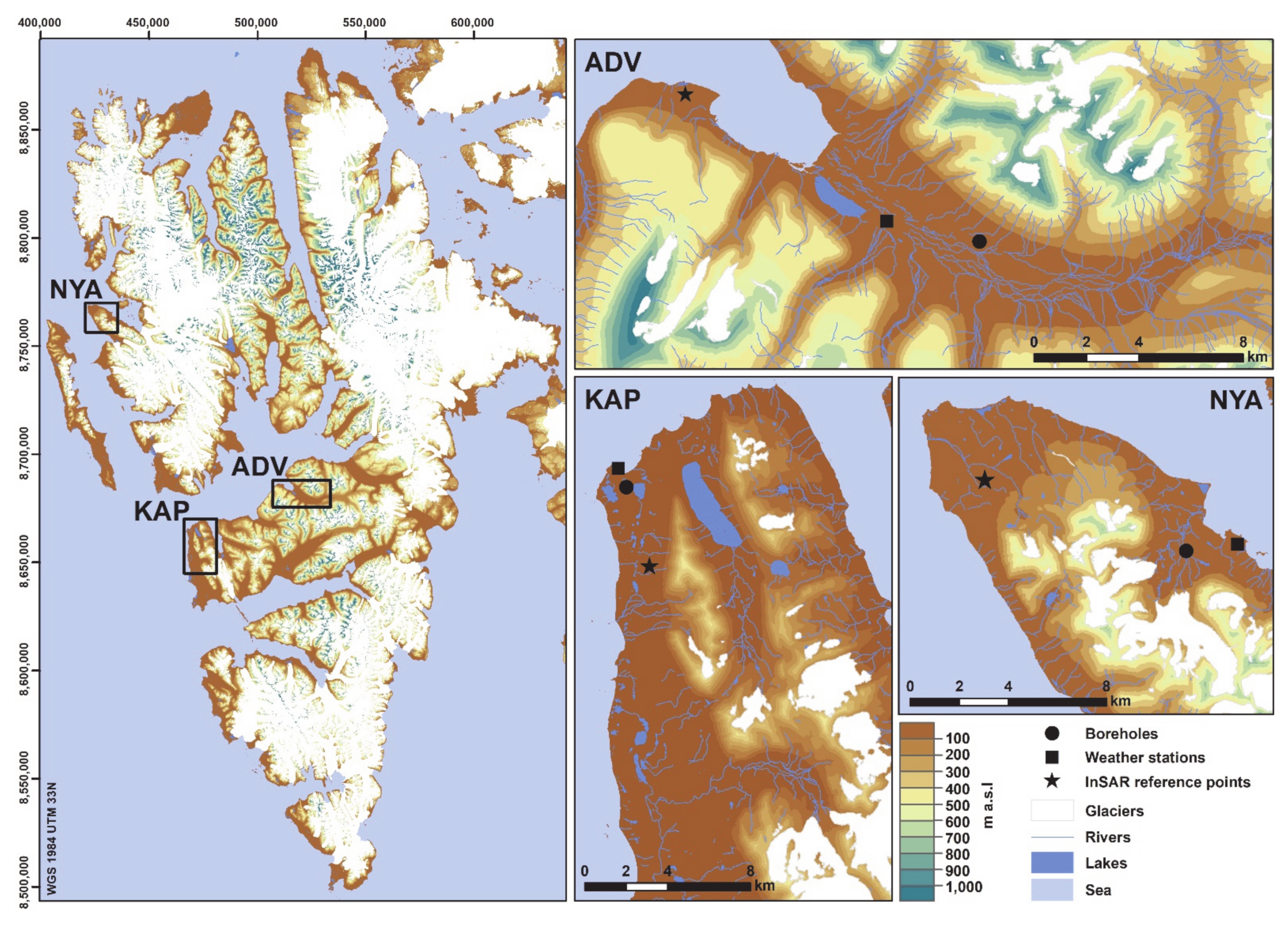
2. Study Areas
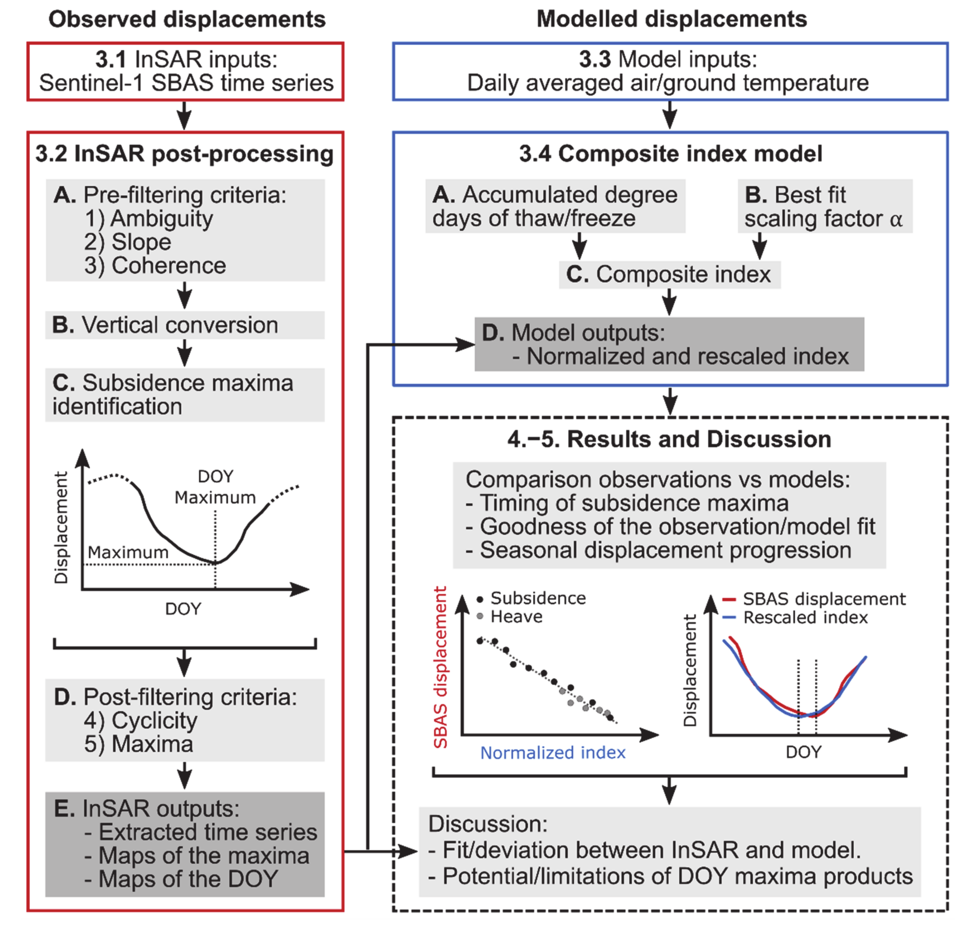
3. Data and Methods
3.1. Sentinel-1 SBAS Time Series
3.2. InSAR Post-Processing and Identification of the Thaw Subsidence Maxima
- A.
- Pre-filtering of the initial SBAS results:
- Criterion 1 “Ambiguity”: InSAR signal becomes aliased when the displacement gradient between adjacent pixels is higher than a quarter of the wavelength during the selected time interval. When using Sentinel-1 (5.6 cm wavelength), if the displacement is over 14 mm between the acquisitions used to build interferograms, there is a higher probability of spatial phase unwrapping error [69]. We therefore filtered out the results likely to be affected by a phase unwrapping error by filtering out pixels including a displacement gradient over 14 mm between successive acquisitions of the time series. If the displacement difference is over the ambiguity threshold, for example between the first acquisition (June 22) and the second (28 June), the pixel is discarded.
- Criterion 2 “Slope angle”: Creep processes on slopes are likely to mask out the transition from subsidence to heave due to a gradual and continuous downslope displacement component. Based on a 20 m DEM [47], we computed the slope angle using ArcGIS (©ESRI). We discarded all pixels with slope angle >1.5°, to focus on flat areas (Supplement S4). Solifluction can occur on low-inclined surfaces, and has been reported on 2° slopes [77]. The conservative threshold of 1.5° was used to account for the relatively low DEM resolution, likely to underestimate local slope variabilities.
- Criterion 3 “Coherence”: Decorrelation sources due to snow, ground moisture and vegetation may affect the quality of the displacement estimates [78]. We applied a secondary coherence thresholding more conservative than at the processing stage (Section 3.1). Pixels with mean coherence <0.55 based on the selected interferograms (Table 1; Supplement S1–S3) were discarded.
- B.
- Vertical conversion: InSAR measurements are intrinsically one-dimensional, along the oblique LOS (Table 1) and therefore provide ambiguous information in complex topography, especially if the movement orientation is spatially heterogeneous and/or temporally variable. As we focus here on flat areas, we can assume that all displacements occur vertically (subsidence and heave). Although some local areas (e.g., coastal areas affected by erosion) may slightly deviate from this general assumption, we expect that the dominant ground behaviour at the landscape scale is along the vertical. Therefore, we converted all results from LOS to vertical displacement using the following equation:where Vdisp is the vertical displacement, LOSdisp is the LOS-projected displacement, and Ia is the incidence angle of the radar beam (Table 1). Vdisp documents a subsidence (positive value) or a heave (negative value), relatively to the first acquisition date.
- C.
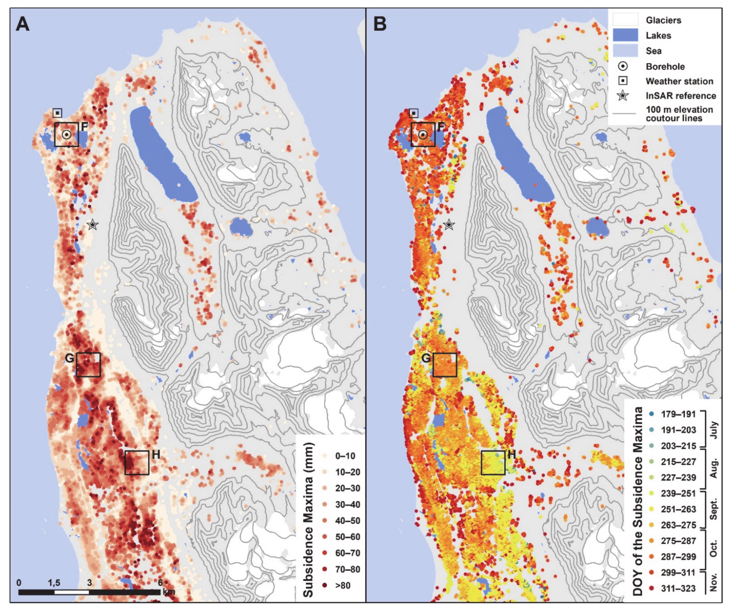
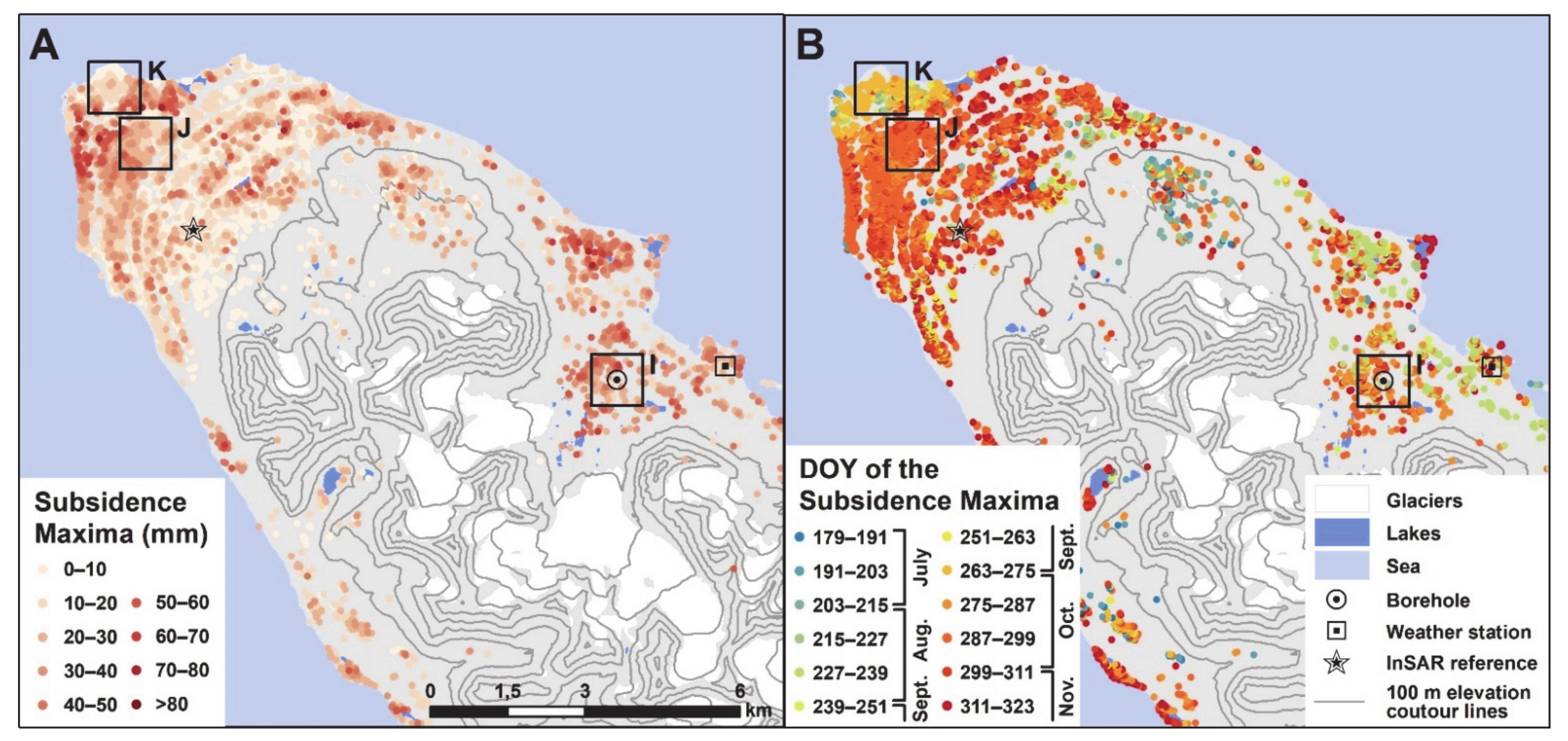
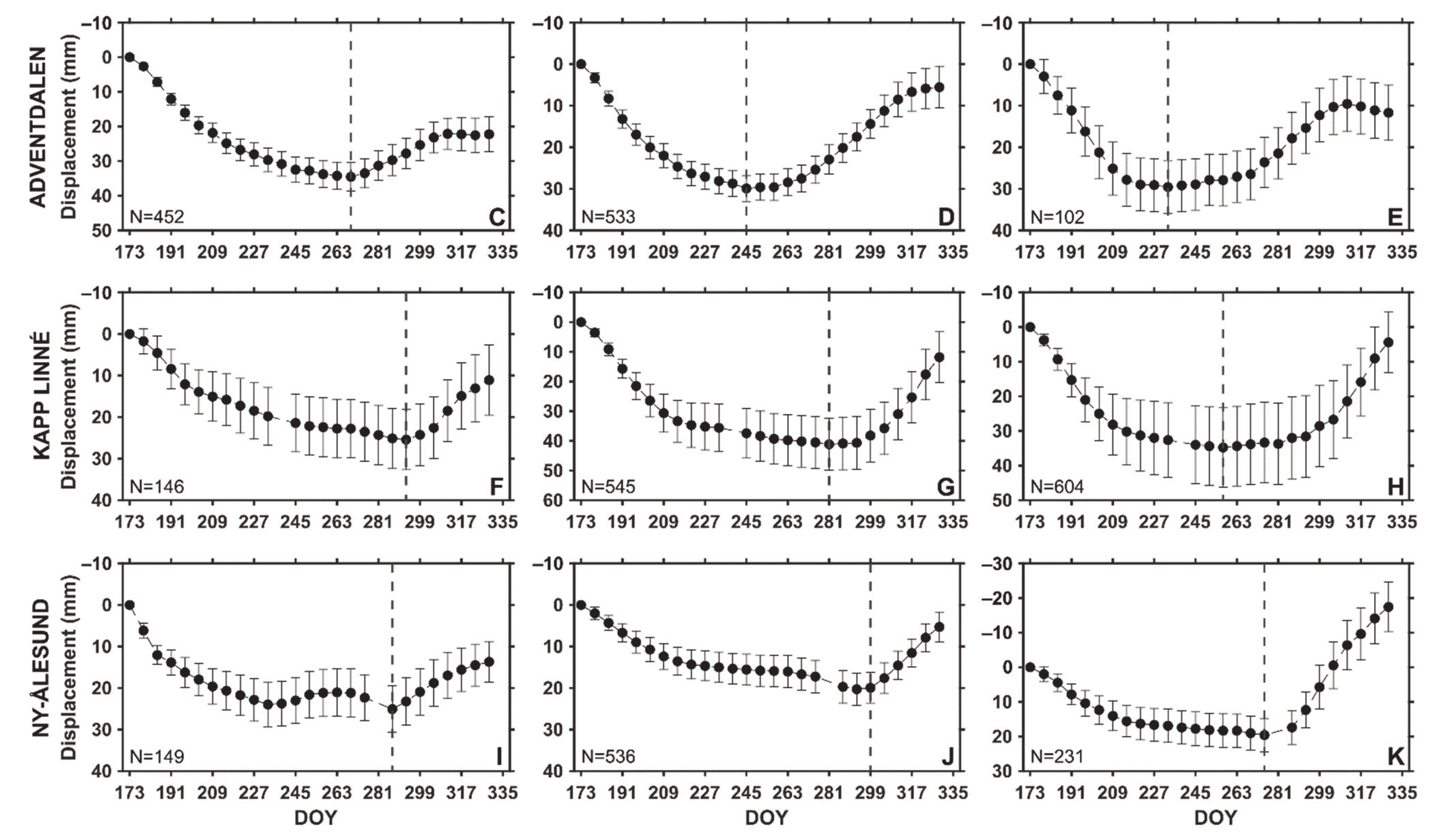
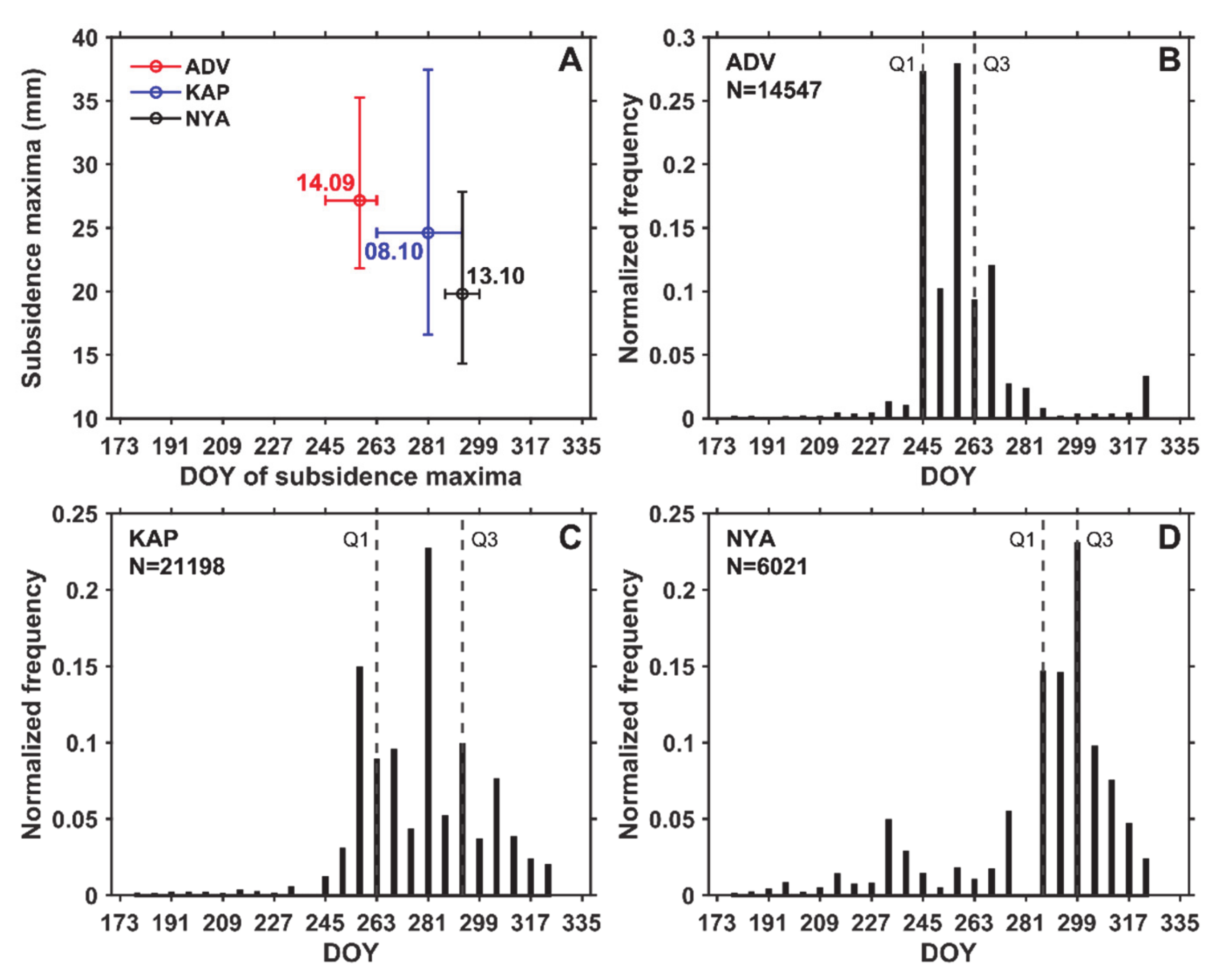
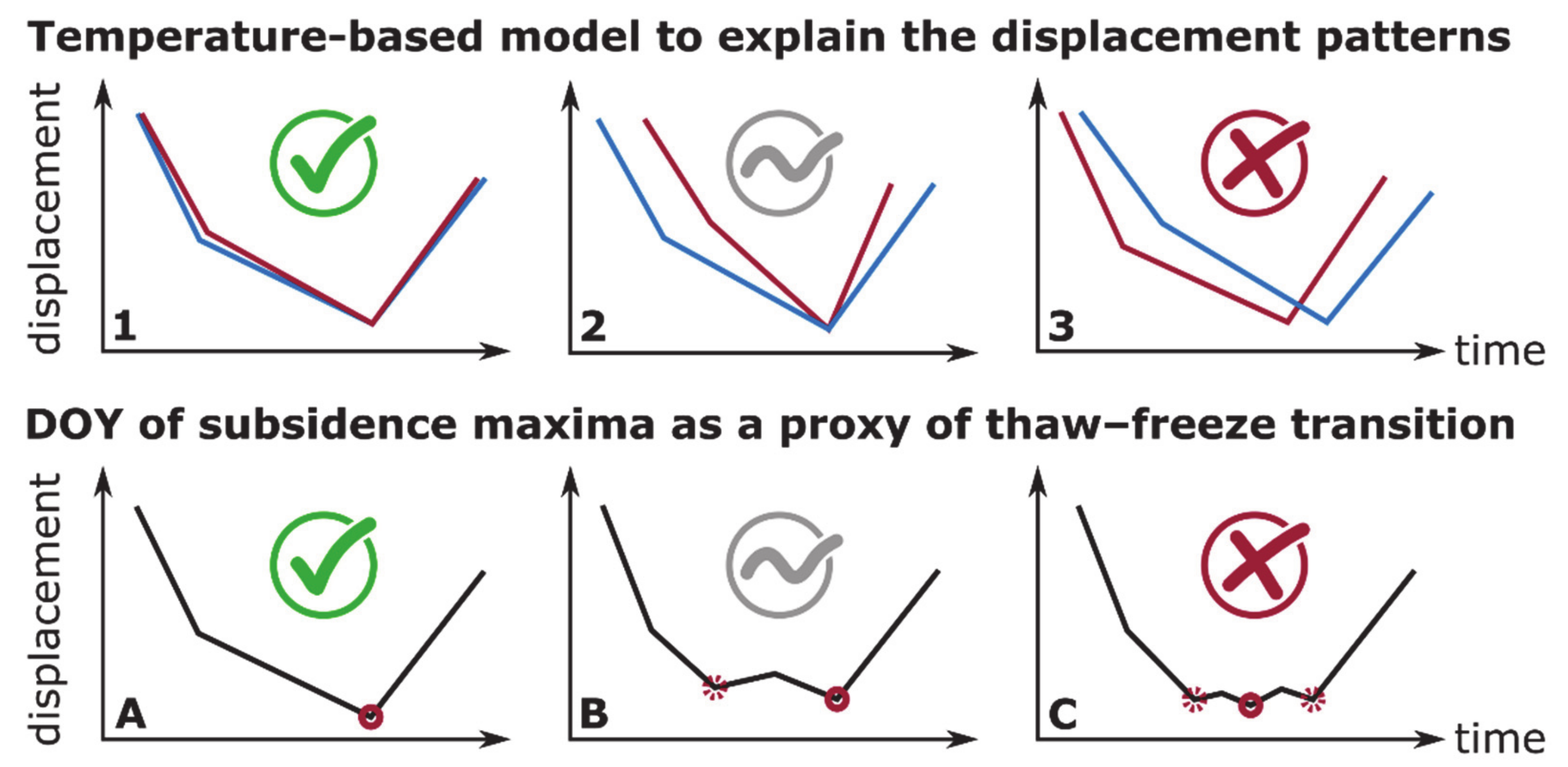
- Subsidence maxima identification: For each time series, the maximal value was identified, and its corresponding Day of Year (DOY) was extracted. It should be noted that the DOY identification is based on the subsidence maximum only and does not take into account the entire pattern of the displacement progression, which may lead to erroneous value if the ground level flattens at the end of the thawing season.
- D.
- Post-filtering of the selected time series:
- Criterion 4 “Cyclicity”: Pixels with DOY corresponding to the first or the last acquisition of the series (i.e., without any subsidence/heave pattern) were discarded, as they do not document a cyclic process. We assume that these pixels correspond to remaining low-inclined areas affected by downslope creep. In combination with Criterion 2 “Slope angle”, Criterion 4 is an additional way to ensure that we focus the analysis on flat areas dominated by vertical patterns.
- Criterion 5 “Maxima”: All pixels with a maximal subsidence <10 mm were additionally discarded, as we assume that the transition between subsidence to heave in areas with low displacement amplitude is likely to be masked out by noise sources (e.g., atmospheric effects, bias due to snow or ground moisture). The temporal resolution of the DOY product is 6 days (12 days when there is one missing acquisition), corresponding the repeat-pass interval of the Sentinel-1 mission.
- E.
- InSAR outputs: For analysing the spatial distribution of the maximal subsidence, we used the results after the four first steps of filtering (Criteria 1−4), while all five criteria are used to map the DOY. For further comparison with the temperature-based model (Section 3.3 and Section 3.4), we focused on time series at three different scales (local, intermediate and regional) by:
- Extracting the nearest pixels to the boreholes;
- Averaging the series for the pixels within 1 km2 around the boreholes;
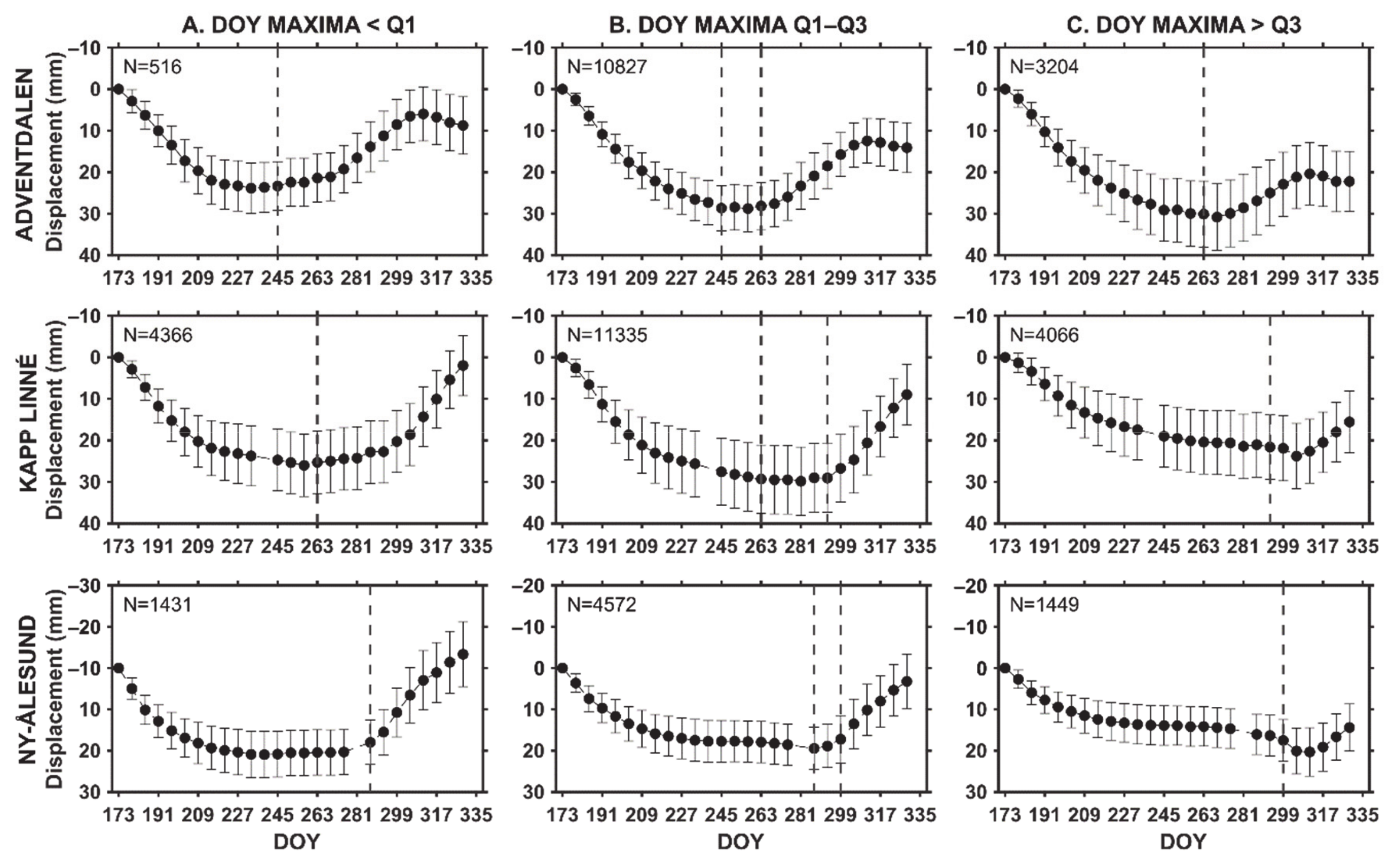
- Averaging the pixels with a DOY of the subsidence maxima within the interquartile range of all results, as we assume that they are representative of the ground behaviour at the regional scale.
When averaging time series, the dispersion of the selected values can be represented by the standard deviation around the mean of the selected pixels for each acquisition date.
3.3. Air and Ground Surface Temperature
3.4. Composite Index Model of Seasonal Time Series
- A.
- B.
- The two seasonal coefficients EF and ET can be related by a scaling factor α:Where kF and kT are the thermal conductivities of the frozen (F) and thawed (T) ground and nF and nT are the n-factors nF and nT as described in Equation (2).
- C.
- Based on Equations (3) and (4), the composite index Ic can be expressed as:
- D.
- Because we are only interested in characterizing the temporal pattern of ground displacements, we normalized the composite index with its maximum value and rescaled it by multiplying the index by the maximal value of the SBAS displacement time series:
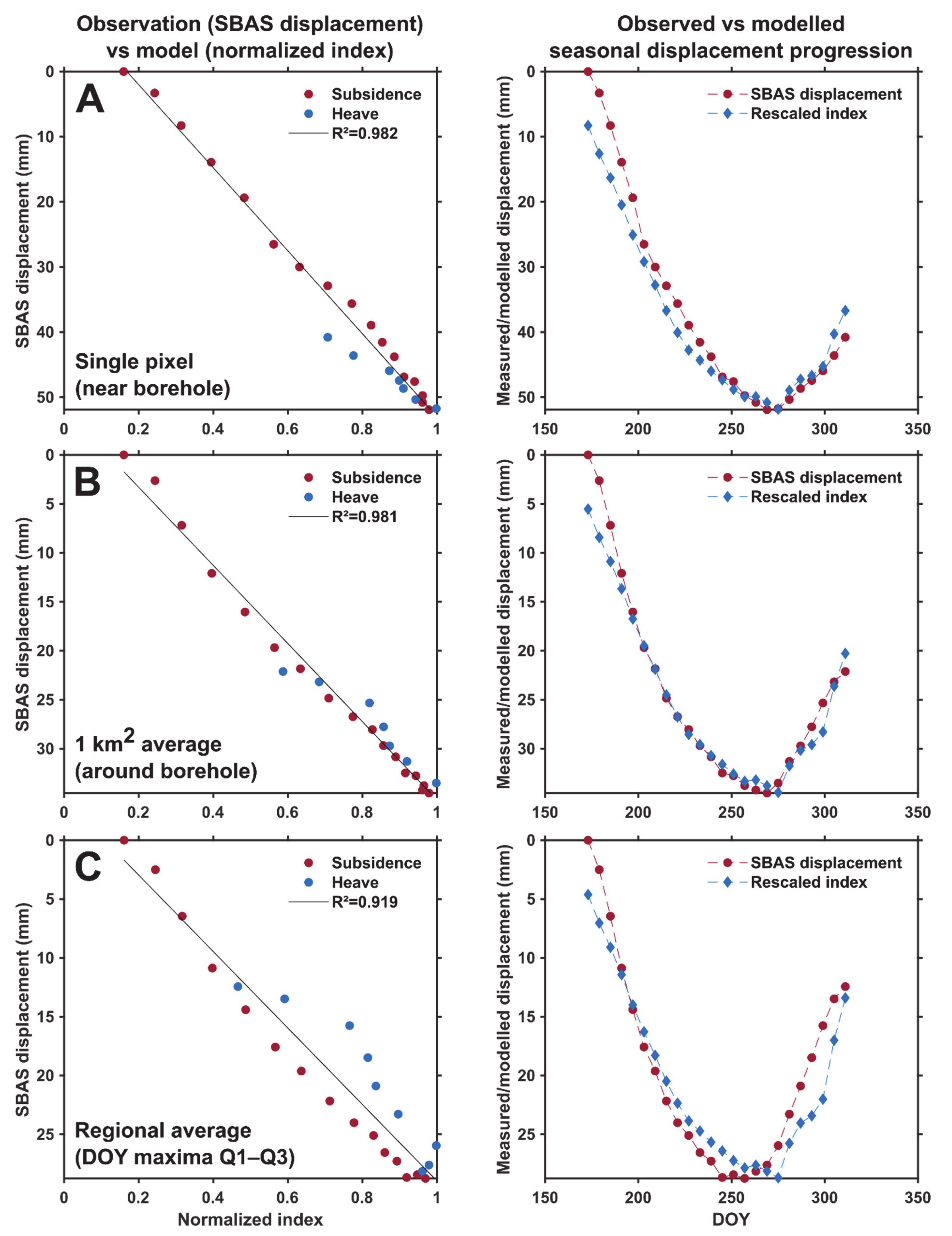
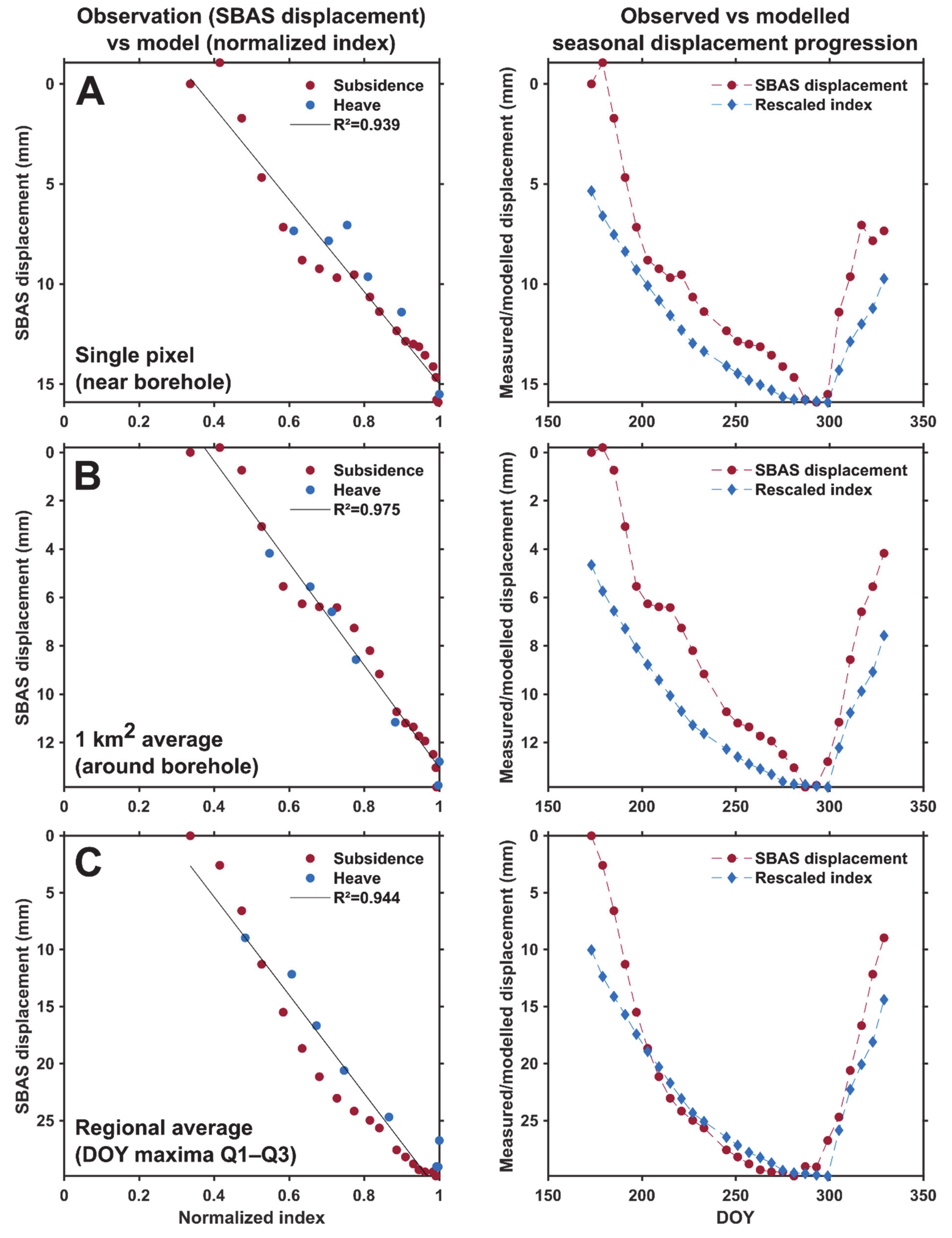
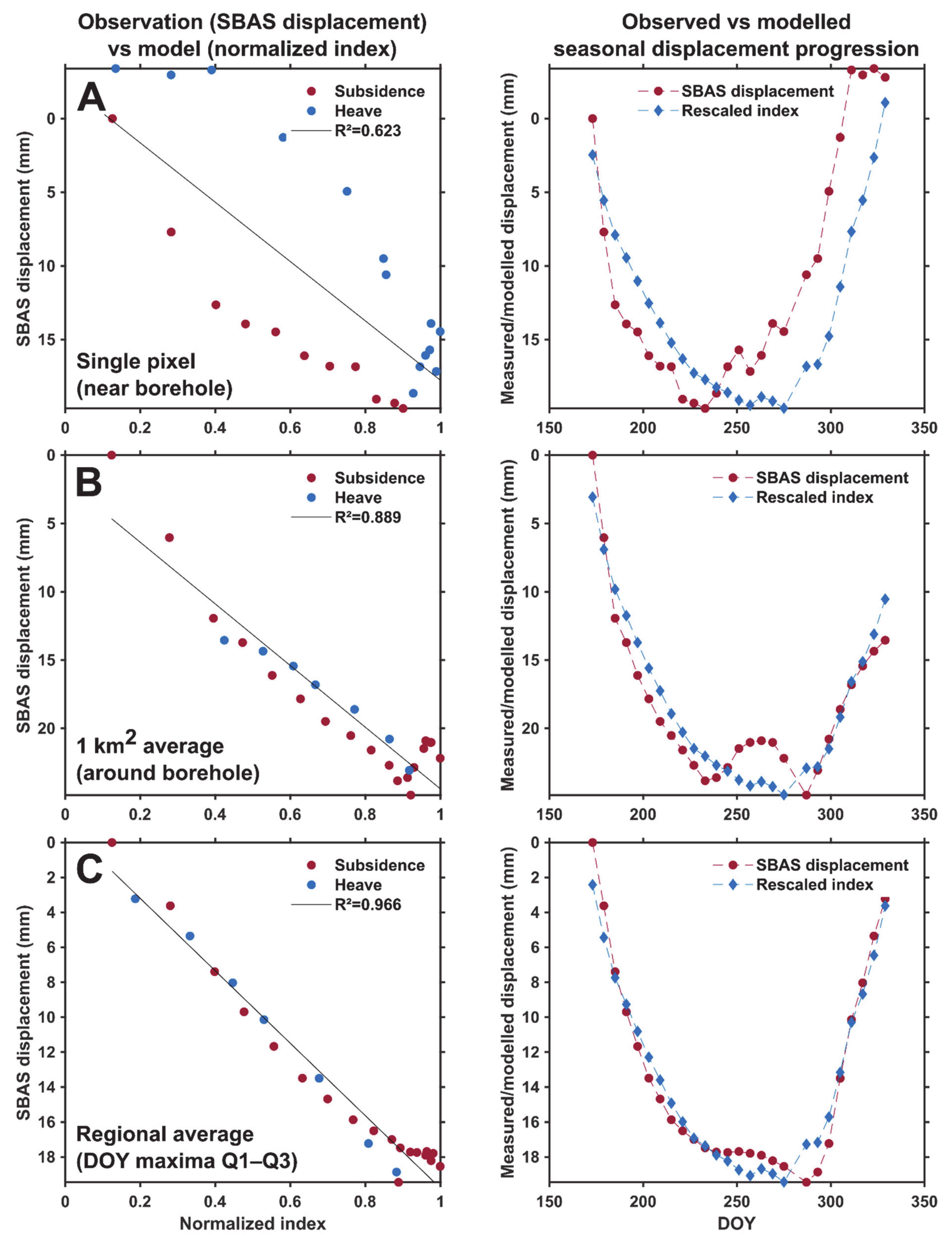
- Comparing the timing of the transition between the subsidence and the heave from the observations and the thawing and freezing periods from the models;
- Evaluating the goodness of the fit between the observations and the models by documenting the proportion of the variance of the seasonal SBAS displacements that is explained by the normalized index (R2);
- Analysing the temporal variations of the entire observed displacement time series with respect to the rescaled composite index;
- Discussing the results’ differences when using air or ground surface temperature, as well as single pixels closest to the boreholes, 1-km2 or regional averaged displacement time series.
4. Results
4.1. Thaw Subsidence Maxima
4.2. Composite Index Model of Seasonal Time Series
5. Discussion
5.1. Seasonal Displacement Patterns
5.2. InSAR Products as Proxy of the Active Layer Thermal Regime
- InSAR processing: The InSAR procedure is currently based on a site-dependent selection of interferograms that include several manual steps (Section 3.1). The variability of the snow cover is the main challenge that can lead to spatially and temporally discontinuous coherent interferometric signals (such as in NYA). Applying automated adaptive filtering, possibly based on a combination of SAR backscatter, InSAR coherence and external meteorological information would be valuable to upscale the procedure, for example to the entire glacier-free land of the Svalbard archipelago. Instead of exploiting similar acquisitions in areas with variable climatic conditions, adaptive InSAR observation windows would allow for the selection of locally relevant periods, starting from the first snow-free scene after thaw onset, and thus avoiding an underestimation of the total seasonal subsidence values (such as in ADV and KAP, Figure 9A).
- DOY extraction: To identify more robustly the timing of the transition between thawing and freezing seasons and solve the issue related to the late-summer flattening of the displacement curves visible in some time series (Figure 13, scenario C), more sophisticated procedures could be tested, for instance by fitting a polynomial function to the entire time series and/or by analysing the displacement gradients between acquisitions, in addition or instead of simply considering the maximal value of the InSAR time series. Scenarios where primary and secondary maxima are identified could also be valuable to further study the cases of summer heave patterns (Figure 13, scenario B).
- Time series averaging: While single time series may be affected by errors or unrepresentative local phenomena (Figure 11A and Figure 12A), the results in KAP and NYA suggest that averaging reduces the noise level and dampens the effect of specific small-scale effects to focus on the main climate-controlled trends. Kilometric averaging may be favoured in future product development, to keep documenting spatial variability while providing more robust information about the general seasonal pattern. At this scale, InSAR processing could be performed with larger multi-looking factors to provide more robust phase statistics for each pixel. Kilometric averaged displacement time series can easily be compared and coupled with transient modelling of thermal conditions based on remotely sensed surface temperature at a similar resolution [11,90]. Comparing InSAR with modelled temperature would have the advantage of increasing the measurement density compared to weather stations and boreholes and could provide new insights on the causes of the spatial-temporal variability of the time series. Moreover, InSAR products could complement and potentially constrain the current permafrost models by indirectly documenting the variability of the ground ice content and the timing of active layer freeze/thaw at a fine resolution and a large scale.
- Time series modelling: To further evaluate the factors controlling the seasonal progression of the displacements in permafrost regions, InSAR observations could be compared with modelled time series based on a variable set of parameters. The composite index model applied in this study is based on the Stefan equation, with simplistic assumptions regarding the ground properties that can explain that the model fails to represent the measurements in several cases (Figure 13, scenarios 2 and 3). As discussed by Gruber [30], one main issue is related to the assumption of constant water content and absence of liquid water in the frozen layer. The model also assumes that the heave is caused by the volumetric change of pore water turning into pore ice (in-situ water freezing). It does not consider the ice segregation (formation of ice lenses), which is known to be an important factor causing frost heave [5,32,91]. Other formulations using the Leybenzon equation, the Kudryavtsev’s or the Gold and Lachbruch’s models [1,29] could be implemented and compared with InSAR time series. Frost heave models taken into account ice lens formation [92] could also be used to further interpret the InSAR-based displacement patterns and their controls.
6. Conclusions
Supplementary Materials
Author Contributions
Funding
Data Availability Statement
Acknowledgments
Conflicts of Interest
References
- French, H.M. The Periglacial Environment, 3rd ed.; John Wiley & Sons: Hoboken, NJ, USA, 2007. [Google Scholar]
- Schuur, E.A.; McGuire, A.D.; Schädel, C.; Grosse, G.; Harden, J.W.; Hayes, D.J.; Hugelius, G.; Koven, C.D.; Kuhry, P.; Lawrence, D.M. Climate change and the permafrost carbon feedback. Nature 2015, 520, 171–179. [Google Scholar] [CrossRef]
- Hjort, J.; Karjalainen, O.; Aalto, J.; Westermann, S.; Romanovsky, V.E.; Nelson, F.E.; Etzelmüller, B.; Luoto, M. Degrading permafrost puts arctic infrastructure at risk by mid-century. Nat. Commun. 2018, 9, 1–9. [Google Scholar] [CrossRef]
- Jorgenson, M.T.; Racine, C.H.; Walters, J.C.; Osterkamp, T.E. Permafrost degradation and ecological changes associated with a warming climate in Central Alaska. Clim. Chang. 2001, 48, 551–579. [Google Scholar] [CrossRef]
- Rempel, A.W. Formation of ice lenses and frost heave. J. Geophys. Res. Earth Surf. 2007, 112, F02S21. [Google Scholar] [CrossRef]
- Bonnaventure, P.P.; Lamoureux, S.F. The active layer: A conceptual review of monitoring, modelling techniques and changes in a warming climate. Prog. Phys. Geogr. 2013, 37, 352–376. [Google Scholar] [CrossRef]
- Biskaborn, B.K.; Smith, S.L.; Noetzli, J.; Matthes, H.; Vieira, G.; Streletskiy, D.A.; Schoeneich, P.; Romanovsky, V.E.; Lewkowicz, A.G.; Abramov, A. Permafrost is warming at a global scale. Nat. Commun. 2019, 10, 1–11. [Google Scholar] [CrossRef] [PubMed] [Green Version]
- Meredith, M.; Sommerkorn, M.; Cassotta, S.; Derksen, C.; Ekaykin, A.; Hollowed, A.; Kofinas, G.; Mackintosh, A.; Melbourne-Thomas, J.; Muelbert, M.M.C. Chapter 3. Polar regions. In IPCC Special Report on the Ocean and Cryosphere in a Changing Climate; The Intergovernmental Panel on Climate Change: Geneva, Switzerland, 2019. [Google Scholar]
- Nitze, I.; Grosse, G.; Jones, B.M.; Romanovsky, V.E.; Boike, J. Remote sensing quantifies widespread abundance of permafrost region disturbances across the Arctic and Subarctic. Nat. Commun. 2018, 9, 1–11. [Google Scholar] [CrossRef] [PubMed]
- Zhang, T.; Barry, R.G.; Armstrong, R.L. Application of satellite remote sensing techniques to frozen ground studies. Polar Geogr. 2004, 28, 163–196. [Google Scholar] [CrossRef]
- Obu, J.; Westermann, S.; Bartsch, A.; Berdnikov, N.; Christiansen, H.H.; Dashtseren, A.; Delaloye, R.; Elberling, B.; Etzelmüller, B.; Kholodov, A. Northern hemisphere permafrost map based on TTOP modelling for 2000–2016 at 1 km2 scale. Earth Sci. Rev. 2019, 193, 299–316. [Google Scholar] [CrossRef]
- Philipp, M.; Dietz, A.; Buchelt, S.; Kuenzer, C. Trends in satellite earth observation for permafrost related analyses—A review. Remote Sens. 2021, 13, 1217. [Google Scholar] [CrossRef]
- Romanovsky, V.E.; Marchenko, S.S.; Daanen, R.; Sergeev, D.O.; Walker, D.A. Soil climate and frost heave along the permafrost/ecological North American arctic transect. In Proceedings of the 9th International Conference on Permafrost, Fairbanks, Alaska, 29 June–3 July 2008; Volume 2, pp. 1519–1524. [Google Scholar]
- Shiklomanov, N.I.; Streletskiy, D.A.; Little, J.D.; Nelson, F.E. Isotropic thaw subsidence in undisturbed permafrost landscapes. Geophys. Res. Lett. 2013, 40, 6356–6361. [Google Scholar] [CrossRef]
- Bamler, R.; Hartl, P. Synthetic aperture radar interferometry. Inverse Probl. 1998, 14, R1. [Google Scholar] [CrossRef]
- Short, N.; LeBlanc, A.-M.; Sladen, W.; Oldenborger, G.; Mathon-Dufour, V.; Brisco, B. RADARSAT-2 D-InSAR for ground displacement in permafrost terrain, validation from Iqaluit airport, Baffin Island, Canada. Remote Sens. Environ. 2014, 141, 40–51. [Google Scholar] [CrossRef]
- Liu, L.; Zhang, T.; Wahr, J. InSAR measurements of surface deformation over permafrost on the north slope of Alaska. J. Geophys. Res. Earth Surf. 2010, 115, F03023. [Google Scholar] [CrossRef]
- Zwieback, S.; Meyer, F.J. Vulnerable top-of-permafrost ground ice indicated by remotely sensed late-season subsidence. Cryosphere 2020, 15, 2041–2055. [Google Scholar] [CrossRef]
- Daout, S.; Doin, M.-P.; Peltzer, G.; Socquet, A.; Lasserre, C. Large-Scale InSAR monitoring of permafrost freeze-thaw cycles on the Tibetan plateau. Geophys. Res. Lett. 2017, 44, 901–909. [Google Scholar] [CrossRef]
- Bartsch, A.; Leibman, M.; Strozzi, T.; Khomutov, A.; Widhalm, B.; Babkina, E.; Mullanurov, D.; Ermokhina, K.; Kroisleitner, C.; Bergstedt, H. Seasonal progression of ground displacement identified with satellite radar interferometry and the impact of unusually warm conditions on permafrost at the Yamal Peninsula in 2016. Remote Sens. 2019, 11, 1865. [Google Scholar] [CrossRef] [Green Version]
- Rouyet, L.; Lauknes, T.R.; Christiansen, H.H.; Strand, S.M.; Larsen, Y. Seasonal dynamics of a permafrost landscape, Adventdalen, Svalbard, investigated by InSAR. Remote Sens. Environ. 2019, 231, 111236. [Google Scholar] [CrossRef]
- Reinosch, E.; Buckel, J.; Dong, J.; Gerke, M.; Baade, J.; Riedel, B. InSAR time series analysis of seasonal surface displacement dynamics on the Tibetan plateau. Cryosphere 2020, 14, 1633–1650. [Google Scholar] [CrossRef]
- Liu, L.; Jafarov, E.E.; Schaefer, K.M.; Jones, B.M.; Zebker, H.A.; Williams, C.A.; Rogan, J.; Zhang, T. InSAR detects increase in surface subsidence caused by an arctic tundra fire. Geophys. Res. Lett. 2014, 41, 3906–3913. [Google Scholar] [CrossRef]
- Strozzi, T.; Antonova, S.; Günther, F.; Mätzler, E.; Vieira, G.; Wegmüller, U.; Westermann, S.; Bartsch, A. Sentinel-1 SAR interferometry for surface deformation monitoring in low-land permafrost areas. Remote Sens. 2018, 10, 1360. [Google Scholar] [CrossRef] [Green Version]
- Antonova, S.; Sudhaus, H.; Strozzi, T.; Zwieback, S.; Kääb, A.; Heim, B.; Langer, M.; Bornemann, N.; Boike, J. Thaw subsidence of a Yedoma landscape in Northern Siberia, measured in situ and estimated from TerraSAR-X interferometry. Remote Sens. 2018, 10, 494. [Google Scholar] [CrossRef] [Green Version]
- Abe, T.; Iwahana, G.; Efremov, P.V.; Desyatkin, A.R.; Kawamura, T.; Fedorov, A.; Zhegusov, Y.; Yanagiya, K.; Tadono, T. Surface displacement revealed by L-Band InSAR analysis in the Mayya area, Central Yakutia, underlain by continuous permafrost. Earth Planets Space 2020, 72, 1–16. [Google Scholar] [CrossRef]
- Hu, Y.; Liu, L.; Larson, K.M.; Schaefer, K.M.; Zhang, J.; Yao, Y. GPS interferometric reflectometry reveals cyclic elevation changes in thaw and freezing seasons in a permafrost area (Barrow, Alaska). Geophys. Res. Lett. 2018, 45, 5581–5589. [Google Scholar] [CrossRef]
- Stefan, J. Über die theorie der eisbildung, insbesondere über die eisbildung im polarmeere. Ann. Phys. Chem. 1891, 42, 269–286. [Google Scholar] [CrossRef] [Green Version]
- Riseborough, D.W.; Shiklomanov, N.; Etzelmüller, B.; Gruber, S.; Marchenko, S. Recent advances in permafrost modelling. Permafr. Periglac. Process. 2008, 19, 137–156. [Google Scholar] [CrossRef]
- Gruber, S. Ground subsidence and heave over permafrost: Hourly time series reveal interannual, seasonal and shorter-term movement caused by freezing, thawing and water movement. Cryosphere 2020, 14, 1437–1447. [Google Scholar] [CrossRef]
- Romanovsky, V.E.; Osterkamp, T.E. Thawing of the active layer on the coastal plain of the Alaskan arctic. Permafr. Periglac. Process. 1997, 8, 1–22. [Google Scholar] [CrossRef]
- Thomas, H.R.; Cleall, P.; Li, Y.-C.; Harris, C.; Kern-Luetschg, M. Modelling of cryogenic processes in permafrost and seasonally frozen soils. Géotechnique 2009, 59, 173–184. [Google Scholar] [CrossRef]
- Zhao, R.; Li, Z.-W.; Feng, G.-C.; Wang, Q.-J.; Hu, J. Monitoring surface deformation over permafrost with an improved SBAS-InSAR algorithm: With emphasis on climatic factors modeling. Remote Sens. Environ. 2016, 184, 276–287. [Google Scholar] [CrossRef]
- Dehls, J.F.; Larsen, Y.; Marinkovic, P.; Lauknes, T.R.; Stødle, D.; Moldestad, D.A. INSAR.No: A national insar deformation mapping/monitoring service in Norway–from concept to operations. In Proceedings of the IGARSS 2019—IEEE International Geoscience and Remote Sensing Symposium, Yokohama, Japan, 28 July–2 August 2019; pp. 5461–5464. [Google Scholar]
- Larsen, Y.; Marinkovic, P.; Dehls, J.F.; Bredal, M.; Bishop, C.; Jøkulsson, G.; Gjøvik, L.-P.; Frauenfelder, R.; Salazar, S.E.; Vöge, M.; et al. European Ground Motion Service: Service Implementation Plan and Product Specification Document. Copernicus Land Monitoring Service. 2020. Available online: https://land.copernicus.eu/user-corner/technical-library/egms-specification-and-implementation-plan (accessed on 1 March 2021).
- Peel, M.C.; Finlayson, B.L.; McMahon, T.A. Updated world map of the Köppen-Geiger climate classification. Hydrol. Earth Syst. Sci. 2007, 11, 1633–1644. [Google Scholar] [CrossRef] [Green Version]
- Harland, W.B. Svalbard. In The Geology of Svalbard; Geological Society: London, UK, 1997; Volume 17, pp. 3–15. [Google Scholar]
- Hanssen-Bauer, I.; Førland, E.J.; Hisdal, H.; Mayer, S.; AB, S.; Sorteberg, A. Climate in Svalbard 2100; NCCS Report no. 1/2019; Norwegian Centre for Climate Services (NCCS): Trondheim, Norway; Norwegian Environment Agency (Miljødirektoratet): Trondheim, Norway, 2019. [Google Scholar]
- Humlum, O.; Instanes, A.; Sollid, J.L. Permafrost in Svalbard: A review of research history, climatic background and engineering challenges. Polar Res. 2003, 22, 191–215. [Google Scholar] [CrossRef] [Green Version]
- Christiansen, H.H.; Humlum, O.; Eckerstorfer, M. Central Svalbard 2000–2011 meteorological dynamics and periglacial landscape response. Arct. Antarct. Alp. Res. 2013, 45, 6–18. [Google Scholar] [CrossRef] [Green Version]
- Harris, C.; Kern-Luetschg, M.; Christiansen, H.H.; Smith, F. The role of interannual climate variability in controlling solifluction processes, Endalen, Svalbard. Permafr. Periglac. Process. 2011, 22, 239–253. [Google Scholar] [CrossRef]
- Schuh, C.; Frampton, A.; Christiansen, H.H. Soil moisture redistribution and its effect on inter-annual active layer temperature and thickness variations in a dry loess terrace in Adventdalen, Svalbard. Cryosphere 2017, 11, 635–651. [Google Scholar] [CrossRef] [Green Version]
- Christiansen, H.H.; Etzelmüller, B.; Isaksen, K.; Juliussen, H.; Farbrot, H.; Humlum, O.; Johansson, M.; Ingeman-Nielsen, T.; Kristensen, L.; Hjort, J. The thermal state of permafrost in the Nordic area during the international polar year 2007–2009. Permafr. Periglac. Process. 2010, 21, 156–181. [Google Scholar] [CrossRef] [Green Version]
- Christiansen, H.H.; Gilbert, G.L.; Neumann, U.; Demidov, N.; Guglielmin, M.; Isaksen, K.; Osuch, M.; Boike, J. Ground ice content, drilling methods and equipment and permafrost dynamics in Svalbard 2016–2019 (PermaSval). In The State of Environmental Science in Svalbard (SESS Report 2020); Svalbard Integrated Arctic Earth Observing System: Svalbard, Norway, 2021. [Google Scholar]
- Strand, S.M.; Christiansen, H.H.; Johansson, M.; Åkerman, J.; Humlum, O. Active layer thickening and controls on interannual variability in the Nordic arctic compared to the circum-arctic. Permafr. Periglac. Process. 2020, 32, 47–58. [Google Scholar] [CrossRef]
- Etzelmüller, B.; Schuler, T.V.; Isaksen, K.; Christiansen, H.H.; Farbrot, H.; Benestad, R. Modeling the temperature evolution of Svalbard permafrost during the 20th and 21st Century. Cryosphere 2011, 5, 67–79. [Google Scholar] [CrossRef] [Green Version]
- NPI Terrengmodell Svalbard (S0 Terrengmodell) [Dataset]. Norwegian Polar Institute. 2014. Available online: https://www.doi.org/10.21334/npolar.2014.dce53a47 (accessed on 1 March 2021).
- NPI Kartdata Svalbard 1:100 000 (S100 Kartdata)/Map Data [Dataset]. Norwegian Polar Institute. 2014. Available online: https://www.doi.org/10.21334/npolar.2014.645336c7 (accessed on 1 March 2021).
- Major, H.; Haremo, P.; Dallmann, W.K.; Andresen, A.; Salvigsen, O. Geological Map of Svalbard 1: 100,000, Sheet C9G Adventdalen; Norwegian Polar Institute: Tromsø, Norway, 2001. [Google Scholar]
- Tolgensbakk, J.; Sørbel, L.; Høgard, K. Geomorphological and Quaternary Geological Map of Svalbard 1: 100,000. Sheet C9Q Adventdalen. Temakart 31; Norwegian Polar Institute: Tromsø, Norway, 2001. [Google Scholar]
- Humlum, O. Holocene permafrost aggradation in Svalbard. Geol. Soc. Lond. Spec. Publ. 2005, 242, 119–129. [Google Scholar] [CrossRef]
- Gilbert, G.L.; O’Neill, H.B.; Nemec, W.; Thiel, C.; Christiansen, H.H.; Buylaert, J.-P. Late quaternary sedimentation and permafrost development in a Svalbard Fjord-Valley, Norwegian high arctic. Sedimentology 2018, 65, 2531–2558. [Google Scholar] [CrossRef]
- Cable, S.; Elberling, B.; Kroon, A. Holocene permafrost history and cryostratigraphy in the high-arctic Adventdalen Valley, Central Svalbard. Boreas 2018, 47, 423–442. [Google Scholar] [CrossRef]
- Retelle, M.; Christiansen, H.H.; Hodson, A.; Nikulina, A.; Osuch, M.; Poleshuk, K.; Romashova, K.; Roof, S.; Rouyet, L.; Strand, S.M. Environmental monitoring in the Kapp Linne-Gronfjorden Region (KLEO). In The State of Environmental Science in Svalbard (SESS Report 2019); Svalbard Integrated Arctic Earth Observing System: Longyearbyen, Norway, 2020. [Google Scholar]
- Dallmann, W.K. Geoscience Atlas of Svalbard; Norwegian Polar Institute: Tromsø, Norway, 2015. [Google Scholar]
- Landvik, J.Y.; Landvik, J.Y.; Salvigsen, O. The late Weichselian and Holocene shoreline displacement on the West-Central coast of Svalbard. Polar Res. 1987, 5, 29–44. [Google Scholar] [CrossRef]
- Ohta, Y.; Hjelle, A. Geological Map Svalbard 1: 100,000. Isfjorden: Spitsbergen. Sheet B9G; Norwegian Polar Institute: Oslo, Norway, 1992. [Google Scholar]
- Snyder, J.A.; Werner, A.; Miller, G.H. Holocene cirque glacier activity in Western Spitsbergen, Svalbard: Sediment records from proglacial Linnévatnet. Holocene 2000, 10, 555–563. [Google Scholar] [CrossRef]
- Åkerman, H.J. Relations between slow slope processes and active-layer thickness 1972–2002, Kapp Linné, Svalbard. Nor. Geogr. Tidsskr. Nor. J. Geogr. 2005, 59, 116–128. [Google Scholar] [CrossRef]
- Eckerstorfer, M.; Malnes, E.; Christiansen, H.H. Freeze/Thaw conditions at periglacial landforms in Kapp Linné, Svalbard, investigated using field observations, in situ, and radar satellite monitoring. Geomorphology 2017, 293, 433–447. [Google Scholar] [CrossRef]
- Hjelle, A. Geological Map of Svalbard 1: 100,000: Sheet A7G Kongsfjorden; Norwegian Polar Institute: Tromsø, Norway, 1999. [Google Scholar]
- Miccadei, E.; Piacentini, T.; Berti, C. Geomorphological features of the Kongsfjorden area: Ny-Ålesund, Blomstrandøya (NW Svalbard, Norway). Rend. Lincei 2016, 27, 217–228. [Google Scholar] [CrossRef]
- Westermann, S.; Langer, M.; Boike, J. Spatial and temporal variations of summer surface temperatures of high-arctic tundra on Svalbard—Implications for MODIS LST based permafrost monitoring. Remote Sens. Environ. 2011, 115, 908–922. [Google Scholar] [CrossRef]
- Boike, J.; Roth, K.; Ippisch, O. Seasonal snow cover on frozen ground: Energy balance calculations of a permafrost site near Ny-Ålesund, Spitsbergen. J. Geophys. Res. Atmos. 2003, 108, ALT-4. [Google Scholar] [CrossRef] [Green Version]
- Westermann, S.; Wollschläger, U.; Boike, J. Monitoring of active layer dynamics at a permafrost site on Svalbard using multi-channel ground-penetrating radar. Cryosphere 2010, 4, 475–487. [Google Scholar] [CrossRef] [Green Version]
- Boike, J.; Juszak, I.; Lange, S.; Chadburn, S.; Burke, E.; Overduin, P.P.; Roth, K.; Ippisch, O.; Bornemann, N.; Stern, L. A 20-year record (1998–2017) of permafrost, active layer and meteorological conditions at a high arctic permafrost research site (Bayelva, Spitsbergen). Earth Syst. Sci. Data 2018, 10, 355–390. [Google Scholar] [CrossRef] [Green Version]
- Larsen, Y.; Engen, G.; Lauknes, T.R.; Malnes, E.; Høgda, K.A. A generic differential interferometric SAR processing system, with applications to land subsidence and snow-water equivalent retrieval. In Proceedings of the ESA Fringe Workshop, Frascati, Italy, 28 November–2 December 2005. [Google Scholar]
- Baran, I.; Stewart, M.P.; Kampes, B.M.; Perski, Z.; Lilly, P. A modification to the Goldstein radar interferogram filter. IEEE Trans. Geosci. Remote Sens. 2003, 41, 2114–2118. [Google Scholar] [CrossRef] [Green Version]
- Goldstein, R.M.; Werner, C.L. Radar interferogram filtering for geophysical applications. Geophys. Res. Lett. 1998, 25, 4035–4038. [Google Scholar] [CrossRef] [Green Version]
- Cavalié, O.; Doin, M.-P.; Lasserre, C.; Briole, P. Ground motion measurement in the lake Mead area, Nevada, by differential synthetic aperture radar interferometry time series analysis: Probing the lithosphere rheological structure. J. Geophys. Res. Solid Earth 2007, 112, B03403. [Google Scholar] [CrossRef] [Green Version]
- Lauknes, T.R. InSAR tropospheric stratification delays: Correction using a small baseline approach. IEEE Geosci. Remote Sens. Lett. 2011, 8, 1070–1074. [Google Scholar] [CrossRef]
- Tymofyeyeva, E.; Fialko, Y. Mitigation of atmospheric phase delays in InSAR data, with application to the Eastern California shear zone. J. Geophys. Res. Solid Earth 2015, 120, 5952–5963. [Google Scholar] [CrossRef]
- Chen, C.W.; Zebker, H.A. Phase unwrapping for large SAR interferograms: Statistical segmentation and generalized network models. IEEE Trans. Geosci. Remote Sens. 2002, 40, 1709–1719. [Google Scholar] [CrossRef] [Green Version]
- NPI Data and Services. Svalbard Orthophoto—WMTS Basemap Service. Norwegian Polar Institute. 2021. Available online: https://geodata.npolar.no/ (accessed on 10 March 2021).
- Berardino, P.; Fornaro, G.; Lanari, R.; Sansosti, E. A new algorithm for surface deformation monitoring based on small baseline differential SAR interferograms. IEEE Trans. Geosci. Remote Sens. 2002, 40, 2375–2383. [Google Scholar] [CrossRef] [Green Version]
- Lauknes, T.R.; Zebker, H.A.; Larsen, Y. InSAR deformation time series using an L1-norm small-baseline approach. IEEE Trans. Geosci. Remote Sens. 2010, 49, 536–546. [Google Scholar] [CrossRef] [Green Version]
- Matsuoka, N. Solifluction rates, processes and landforms: A global review. Earth Sci. Rev. 2001, 55, 107–134. [Google Scholar] [CrossRef]
- Zwieback, S.; Liu, X.; Antonova, S.; Heim, B.; Bartsch, A.; Boike, J.; Hajnsek, I. A statistical test of phase closure to detect influences on DInSAR deformation estimates besides displacements and decorrelation noise: Two case studies in high-latitude regions. IEEE Trans. Geosci. Remote Sens. 2016, 54, 5588–5601. [Google Scholar] [CrossRef]
- NCCS. 2017 Daily Air Temperature. Adventdalen Station 99870. Isfjord Radio Station 99790. Ny-Ålesund Station 99910. Norwegian Centre for Climate Services. 2021. Available online: https://seklima.met.no/observations/ (accessed on 30 March 2021).
- Riseborough, D.W. Thawing and freezing indices in the active layer. In Proceedings of the 8th International Conference on Permafrost, Zurich, Switzerland, 21–25 July 2003; Volume 2, pp. 953–958. [Google Scholar]
- Hallet, B.; Allard, M. Measurement of soil motion in sorted circles, Western Spitsbergen. In Proceedings of the 7th International Conference on Permafrost, Yellowknife, Canada, 23–27 June 1998; pp. 415–420. [Google Scholar]
- Matsuoka, N.; Hirakawa, K. Solifluction resulting from one-sided and two-sided freezing: Field data from Svalbard. Polar Geosci. 2000, 13, 187–201. [Google Scholar]
- Watanabe, T.; Matsuoka, N.; Christiansen, H.H. Mudboil and ice-wedge dynamics investigated by electrical resistivity tomography, ground temperatures and surface movements in Svalbard. Geogr. Ann. Ser. A Phys. Geogr. 2012, 94, 445–457. [Google Scholar] [CrossRef]
- Chen, J.; Wu, Y.; O’Connor, M.; Cardenas, M.B.; Schaefer, K.; Michaelides, R.; Kling, G. Active layer freeze-thaw and water storage dynamics in permafrost environments inferred from InSAR. Remote Sens. Environ. 2020, 248, 112007. [Google Scholar] [CrossRef]
- Rudy, A.C.A.; Lamoureux, S.F.; Treitz, P.; Short, N.; Brisco, B. Seasonal and multi-year surface displacements measured by DInSAR in a high arctic permafrost environment. Int. J. Appl. Earth Obs. Geoinf. 2018, 64, 51–61. [Google Scholar] [CrossRef]
- Mackay, J.R. Downward water movement into frozen ground, Western Arctic Coast, Canada. Can. J. Earth Sci. 1983, 20, 120–134. [Google Scholar] [CrossRef]
- Romanovsky, V.E.; Sazonova, T.S.; Balobaev, V.T.; Shender, N.I.; Sergueev, D.O. Past and recent changes in air and permafrost temperatures in Eastern Siberia. Glob. Planet. Chang. 2007, 56, 399–413. [Google Scholar] [CrossRef]
- Throop, J.; Lewkowicz, A.G.; Smith, S.L. Climate and ground temperature relations at sites across the continuous and discontinuous permafrost zones, Northern Canada. Can. J. Earth Sci. 2012, 49, 865–876. [Google Scholar] [CrossRef]
- Way, R.G.; Lewkowicz, A.G. Environmental controls on ground temperature and permafrost in Labrador, Northeast Canada. Permafr. Periglac. Process. 2018, 29, 73–85. [Google Scholar] [CrossRef]
- Westermann, S.; Peter, M.; Langer, M.; Schwamborn, G.; Schirrmeister, L.; Etzelmüller, B.; Boike, J. Transient modeling of the ground thermal conditions using satellite data in the Lena River Delta, Siberia. Cryosphere 2017, 11, 1441–1463. [Google Scholar] [CrossRef] [Green Version]
- Smith, M.W. Observations of soil freezing and frost heave at Inuvik, Northwest Territories, Canada. Can. J. Earth Sci. 1985, 22, 283–290. [Google Scholar] [CrossRef]
- Yanagiya, K.; Furuya, M. Post-wildfire surface deformation near Batagay, Eastern Siberia, detected by L-Band and C-Band InSAR. J. Geophys. Res. Earth Surf. 2020, 125, e2019JF005473. [Google Scholar] [CrossRef]
- Karlsen, S.R.; Elvebakk, A.; Høgda, K.A.; Grydeland, T. Spatial and temporal variability in the onset of the growing season on Svalbard, Arctic Norway—Measured by MODIS-NDVI satellite data. Remote Sens. 2014, 6, 8088–8106. [Google Scholar] [CrossRef] [Green Version]
- Vickers, H.; Karlsen, S.R.; Malnes, E. A 20-year MODIS-based snow cover dataset for Svalbard and its link to phenological timing and sea ice variability. Remote Sens. 2020, 12, 1123. [Google Scholar] [CrossRef] [Green Version]


| Land Area [km2] | Selected Number of Interferograms | Line-of-Sight (LOS) Incidence Angle (Ia)/Compass Direction (Di) | Reference Points (UTM 33N) | |
|---|---|---|---|---|
| Adventdalen (ADV) | 307 | 90 | Ia: 37.3°/Di: 69.5° | 8,685,931 511,282 |
| Kapp Linné (KAP) | 288 | 88 | Ia: 34.0°/Di: 67.8° | 8,551,011 469,616 |
| Ny-Ålesund (NYA) | 121 | 84 | Ia: 34.3°/Di: 66.0° | 8,765,916 423,918 |
| Station and Data Types | Coordinates (UTM 33N) | Altitude [m a.s.l] | Site Information and Reference | |
|---|---|---|---|---|
| Adventdalen (ADV) |
Weather station. Air temperature. | 8,681,070 N 518,966 E | 15 | Adventdalen station 99870. Reference: NCCS, 2021 [79]. |
|
Borehole. Ground temperature. |
8,680,294 N 522,504 E | 17 | Ice-wedge polygons in eolian deposit. The area is affected by long-term subsidence, exposing the upper sensors closer to the surface. Data from logger at –23 cm is therefore used in this study, assuming to be representative of the ground surface conditions. The borehole is part of the UNIS monitoring network and temperature data has previously been compared with InSAR in Rouyet et al., 2019 [21]. | |
| Kapp Linné (KAP) |
Weather station. Air temperature. | 8,665,721 N 468,119 E | 7 | Isfjord Radio station 99790. Reference: NCCS, 2021 [79]. |
|
Borehole. Ground temperature. | 8,664,808 N 468512 E | 21 | Beach ridge on strandflat composed of coarse-grained beach sediment. Sensor at ground surface. GTN-P and NORPERM references: NO 36/KL-B-2. Reference: Christiansen et al., 2010; 2021 [43,44]. | |
| Ny-Ålesund (NYA) |
Weather station. Air temperature. | 434,216 N 8,763,255 E | 8 | Ny-Ålesund station 99910. Reference: NCCS, 2021 [79]. |
|
Borehole. Ground temperature. | 8,762,985 N 432,118 E | 25 | Diamict surface with fine-grained glaciofluvial sediments. Profile C. Sensor at –1 cm. GTN-P reference: NO GE 60. Reference: Boike et al., 2018 [66]. |
Publisher’s Note: MDPI stays neutral with regard to jurisdictional claims in published maps and institutional affiliations. |
© 2021 by the authors. Licensee MDPI, Basel, Switzerland. This article is an open access article distributed under the terms and conditions of the Creative Commons Attribution (CC BY) license (https://creativecommons.org/licenses/by/4.0/).
Share and Cite
Rouyet, L.; Liu, L.; Strand, S.M.; Christiansen, H.H.; Lauknes, T.R.; Larsen, Y. Seasonal InSAR Displacements Documenting the Active Layer Freeze and Thaw Progression in Central-Western Spitsbergen, Svalbard. Remote Sens. 2021, 13, 2977. https://doi.org/10.3390/rs13152977
Rouyet L, Liu L, Strand SM, Christiansen HH, Lauknes TR, Larsen Y. Seasonal InSAR Displacements Documenting the Active Layer Freeze and Thaw Progression in Central-Western Spitsbergen, Svalbard. Remote Sensing. 2021; 13(15):2977. https://doi.org/10.3390/rs13152977
Chicago/Turabian StyleRouyet, Line, Lin Liu, Sarah Marie Strand, Hanne Hvidtfeldt Christiansen, Tom Rune Lauknes, and Yngvar Larsen. 2021. "Seasonal InSAR Displacements Documenting the Active Layer Freeze and Thaw Progression in Central-Western Spitsbergen, Svalbard" Remote Sensing 13, no. 15: 2977. https://doi.org/10.3390/rs13152977
APA StyleRouyet, L., Liu, L., Strand, S. M., Christiansen, H. H., Lauknes, T. R., & Larsen, Y. (2021). Seasonal InSAR Displacements Documenting the Active Layer Freeze and Thaw Progression in Central-Western Spitsbergen, Svalbard. Remote Sensing, 13(15), 2977. https://doi.org/10.3390/rs13152977