Article

Automatic Windthrow Detection Using Very-High-Resolution Satellite Imagery and Deep Learning

Botanical Garden-Institute of the Far Eastern Branch of the Russian Academy of Science, Makovskogo St. 142, 690024 Vladivostok, Russia
*
Author to whom correspondence should be addressed.
Remote Sens. 2020, 12(7), 1145; https://doi.org/10.3390/rs12071145
Submission received: 29 February 2020 / Revised: 26 March 2020 / Accepted: 1 April 2020 / Published: 3 April 2020
(This article belongs to the Special Issue Remote Sensing of Natural Forest Disturbances)

Abstract

:
Wind disturbances are significant phenomena in forest spatial structure and succession dynamics. They cause changes in biodiversity, impact on forest ecosystems at different spatial scales, and have a strong influence on economics and human beings. The reliable recognition and mapping of windthrow areas are of high importance from the perspective of forest management and nature conservation. Recent research in artificial intelligence and computer vision has demonstrated the incredible potential of neural networks in addressing image classification problems. The most efficient algorithms are based on artificial neural networks of nested and complex architecture (e.g., convolutional neural networks (CNNs)), which are usually referred to by a common term—deep learning. Deep learning provides powerful algorithms for the precise segmentation of remote sensing data. We developed an algorithm based on a U-Net-like CNN, which was trained to recognize windthrow areas in Kunashir Island, Russia. We used satellite imagery of very-high spatial resolution (0.5 m/pixel) as source data. We performed a grid search among 216 parameter combinations defining different U-Net-like architectures. The best parameter combination allowed us to achieve an overall accuracy for recognition of windthrow sites of up to 94% for forested landscapes by coniferous and mixed coniferous forests. We found that the false-positive decisions of our algorithm correspond to either seashore logs, which may look similar to fallen tree trunks, or leafless forest stands. While the former can be rectified by applying a forest mask, the latter requires the usage of additional information, which is not always provided by satellite imagery.

Graphical Abstract

1. Introduction

Storm winds are the main factor of natural forest damage. Wind disturbances are an important component of forest ecosystem dynamics at different spatial scales [1,2,3,4,5]. It is assumed that global changes can increase the frequency and strength of storms making the impact of winds a more significant factor for forests [6,7,8,9,10,11]. The identification and positioning of windthrow areas along with the essential determination of their areas using satellite imagery are of high importance for purposes of forest management and nature conservation. These problems are also closely related to the carbon balance [12,13], estimation of the fire risk [14], bark beetle outbreaks [15], and management of salvage logging [16,17]. Of particular importance are remote sensing methods in areas with complex terrain and poorly developed infrastructure because such territories are greatly limited with regard to the ability to conduct ground-based surveys.
The commonly used methods for assessing forest disturbances consist of analyzing the multitemporal remote sensing data of pre- and post-disturbance images. For example, this approach is used by the popular forest dynamics service Global Forest Watch [18], which is based on high-resolution global maps of forest cover change [19,20] that are used in a large number of studies around the world. This kind of research widely relies on multispectral imagery from publicly available sources, which are made by means of medium- or high-resolution sensors installed on satellites of the Landsat family, Sentinel-1, Sentinel-2, and others [17,21,22,23,24], as well using very-high-resolution satellite imagery [25]. Although the comparison-based approach has proven its efficacy, it has limitations. For example, each analyzed area to be assessed requires at least two cloudless images from before and after the occurrence of the disturbance event. This is not always possible for territories that are continuously covered by clouds or fogs. Another drawback of this approach is the difficulty in determining the causes of forest disturbances. In addition to storm winds, these causes can include insect disasters, logging, landslides, and avalanches that may look similar and show similar spectral behavior.
The second approach to detecting forest disturbances is to apply artificial intelligence and machine learning algorithms to remote sensing data [26,27,28]. During the last decade, artificial neural networks, especially deep learning algorithms, have shown incredible performance in the analysis and segmentation of images derived from various types of human activities [29,30,31].
In the context of computer vision, several different problems have been identified. These are image classification and segmentation problems, including context segmentation and instance segmentation [32,33]. The former involves the identification of all pixels belonging to the same class on the image (e.g., highlighting all pixels in a photo that correspond to humans), the latter consists of determining all pixels belonging to a specific object on the image (e.g., recognizing each human as a separate object). Significant developments have been observed in addressing all of these computer vision problems thanks to the application and development of neural networks and deep learning [34,35,36]. Deep learning algorithms are being increasingly used in environmental sciences and can be beneficial to most ecological disciplines for a wide range of ecological problems, including applied contexts such as resource management and nature conservation [30]. In the context of vegetation science and forestry, the deep learning approach has high potential and is only at the beginning of its development [37,38]. In the case of the problem in recognition of forest disturbances, there are only a few works discovering peculiarities of solving problems using deep learning methods [39,40,41].
In this study, we consider a class of U-Net-like convolutional neural networks (CNNs) that have shown their efficiency in biomedical image segmentation. U-Net was originally proposed by Ronneberger et al. [42] for segmenting biological microscopy images; it won the International Symposium on Biomedical Imaging (ISBI) cell tracking challenge by a large margin. It is worth noting that U-Net was trained on an extremely small number of images (only 30 microscopy images were used) and heavily relied on data augmentation to learn from the available images more effectively.
Since that time, various U-Net-like CNNs have been developed for different kinds of image segmentation problems. Zhang et al. [43] proposed a road segmentation algorithm based on U-Net. This architecture was extended for handling 3D images by Çiçek et al. [44]. Recently, CNNs demonstrated their efficiency in the windthrow identification problem [39], forest inventory [45], recognition of different vegetation types [46,47] and separate trees [41,48,49].
In our study, we share our experience of using U-Net-like CNNs for recognizing windthrow areas in the dark coniferous forests of Kunashir Island (the Kuril Islands, Russia), which was severely damaged by a storm on 17 December 2014. The mid-latitude cyclone came from Hokkaido Island, Japan, with east-northeast wind gusts of 43 m·s−1 (mean wind speed was recorded as 22 m·s−1) and subsequently moved to the Pacific Ocean. The minimal sea-level atmosphere pressure for the storm event was 971 hPa, and the cumulative precipitation amounted to 28 mm (100 mm layer of wet snow) [50] (https://rp5.ru/Weather_archive_in_Yuzhno-Kurilsk). This study extends upon the experience of using U-Net-like CNNs for problems in windthrow patch recognition areas (the areas covered with uprooted and wind snapped trees), demonstrating the peculiarities of exploiting high-resolution satellite imagery.

2. Materials and Methods
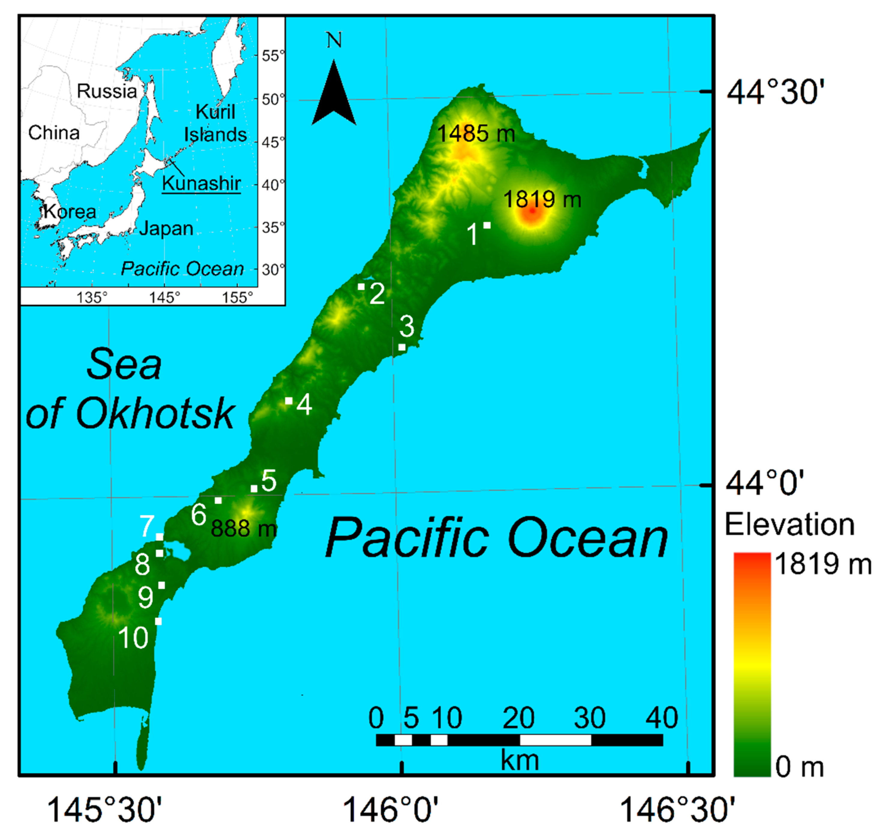
2.1. Study Area

Kunashir is the southern island of the Kuril Islands archipelago (Russia, 44.0°N 145.8°E; Figure 1). The area of Kunashir is almost 1490 km2, whereby the area of forest covered with crown density >30%, is approximately equal to 1210 km2 [19].
Within Kunashir Island, the majority of the forested landscape is characterized by dark and mixed coniferous forests with dominated by Sakhalin fir (Abies sachalinensis (F. Schmidt) Mast.), Yezo spruce (Picea jezoensis (Siebold & Zucc.) Carrière), and Sakhalin spruce (Picea glehnii (F. Schmidt) Mast.). Dark coniferous forest typified by a moderate to closure canopy layer of needle-leaved evergreen trees on average not exceeding 20 m in height. The average diameter at breast height (DBH) of adult trees is 30 cm, with a maximum of more than 70 cm. Broad-leaved cold-deciduous trees may form a scattered subcanopy, particularly in canopy gaps. Stone birch (Betula ermanii Cham.) and Mongolian oak (Quercus mongolica Fisch. ex Ledeb.) stand with an understory layer of dwarf bamboos (Sasa spp.) that encompass the seral forest communities. Stands of this forest typically contain closure canopy (90–100%) cover of not tall trees approaching 10–12 m with DBH less than 20 cm. There is not often a sparse layer of old-growth big birches and oaks with DBH more than 100 cm. Stone birch communities (including krummholz) and Siberian dwarf pine thickets (Pinus pumila (Pall.) Regel) also occupy the subalpine vertical belt in the mountains. In December 2014, a violent storm occurred, characterized by strong winds and high precipitation composed of wet snow caused windthrows in the dark coniferous forests over large areas of the island. We found no wind disturbance in the subalpine forests during our ground-based forest studies and only minor damage in the birch oak forest with dwarf bamboo.

2.2. Satellite Data

Source data were collected from 10 sites in different parts of Kunashir Island. Seven of these fell into the category of forest landscape with different types of forests and include windthrow areas. Three plots did not include forested areas or windthrow patches (Table 1). We used very-high-resolution imagery, without clouds, for all of these sites, which came from the satellites Pleiades-1A/B (five images) and Worldview-3 (one image). The spatial resolution of the pansharpened images obtained from the Pleiades-1A/B satellite sensors was 0.5 m/pixel [51]. These images were provided without atmospheric corrections and encoded in RGB-colorspace (Supplementary Materials, Figures S1–S10). However, due to the relatively cloudy conditions of oceanic climate in the study area, it was impossible to choose all images from only a single satellite camera as this led to images of slightly different quality and resolution. Images of the study sites have a resolution of 2500 × 2500 pixels (~1 km × 1 km on the surface in Pleiades-1A/B images), except for the sites #4 and #9, where the images are smaller and have a resolution of 1250 × 1250 pixels (~500 m × 500 m). Further, these images were used in training and validation datasets by randomly and repeatedly cropping sub-images having a resolution of 256 × 256 pixels (~128 × 128 m).
In addition, we used a specific snapshot by WorldViev-3 with a resolution of 0.31 m/pixel [52]. This snapshot was taken on the same date as most of the Pleiades-1A/B images and did not contain windthrow sites but included patches of leafless subalpine stone birch forests that look very similar to windthrows. It was difficult for non-specialists to make the right delineation in this snapshot without any contextual information about the landscape nor a priori knowledge about the vegetation cover encountered in these types of sites. We used this to demonstrate possible false-positive cases that may be determined when using our approach of windthrow recognition.
We used images dated to 2015 since this corresponds to the first year after the forest wind damage occurred. For such a time span, specific patterns corresponding to windthrow patches were clearly recognized on satellite images. The natural overgrowing of disturbed forest sites by undergrowth and shrubs reduces the possibility of correctly recognizing these areas since the specific pattern of well-recognized fallen tree trunks disappears. Therefore, newly arisen windthrow areas cannot be reliably recognized after several vegetative seasons from the moment when the disturbance event occurred. For the same reason, we used images dated to the beginning of the growing season, with the exception of one part of the island in which cloudless images were available for July 2015.

2.3. Training and Validation Data

To train our model, we manually delineated masks of windthrow sites for all available images (Table 1). Original images and corresponding masks had been read as arrays of different shapes. RGB-images had shape (w, h, 3), where w and h are the number of pixels per width and height, respectively, and 3 is the number of image channels. Pixel-wise labels (mask images) had the same size as corresponding RGB images and differed only by the number of channels (which was equal to 1). The pixel of a mask image was internally assigned as 1 if it belonged to the damaged area and 0 otherwise.
Taking into account the experience of solving similar problems of segmentation of remote sensing data [39], we chose the size of the input image as equal to 256 × 256, which approximately corresponds to a 128 m × 128 m square on the ground for the Pleiades-1A/B images. This size is sufficient to figure out a specific pattern of forest-disturbed areas that is important for neural network training and is not restrictive from the perspective of the required memory.
Training data were generated as batches of size (m, 256, 256, 3), where m is the batch size (m = 20 in our experiments). The batches consisted of sub-images of size 256 × 256 that were randomly cropped out from the original satellite images presented in Table 1. We had a stream (internally, a Python generator) of almost never repeated sub-images; these sub-images were combined into batches and used for the neural network training. Satellite images for sites #1, #3, #5, #7–10 were used for training and #2, #4, #6 for validation. Corresponding batches of mask data had shape (20, 256, 256, 1). The network training assessment was performed on sub-images generated from image #2 (Table 1). Images #4 and #6 were used for visualization and demonstration of the algorithm efficacy.
Augmentation is an important part of the neural network learning process that resolves the problem of overfitting [53,54]. Original satellite images were obtained in different atmospheric conditions and had slightly different values of saturation, so we decided to use a specific augmentation technique to expand the number of training images, and thereby improve the network performance. As an augmentation transformation, we chose random changes of RGB channels of the original images and random vertical and horizontal flips. Random changes for each RGB channel did not exceed 0.1 by absolute value and were applied simultaneously to all channels, as it is implemented in the utility function “apply_channel_shift” from the Keras package [54]. Random flips provided additional variability of images used for training and reduced overfitting. We also considered using small random rotations in the augmentation pipeline. However, adding rotations did not improve the network performance, and we excluded such transformations from the augmentation. It is worth noting that we didn’t use random shifts in the augmentation procedure. Such transformations would be redundant since sub-images were cropped from a fixed set of satellite images and often intersected each other that could be considered as they are spatially shifted.
Therefore, having a batch size of 20 and performing typically up to 1500 epochs for training the network, we used almost 30,000 different augmented images of size 256 × 256.

2.4. Artificial Neural Network Architecture

The problem of forest damage identification is a semantic segmentation problem. Efforts to solve such problems have recently made significant progress due to artificial neural networks of complex architecture, which are closely related to a general term referred to as deep learning [55,56,57].
Semantic segmentation is a pixel-wise classification problem aimed at determining the class of the particular pixel of the image it belongs to. It is usually handled by means of convolutional neural networks (CNNs). As was noted in the introduction, one of such CNNs is U-Net, which is of an encoder-decoder architecture [58].
U-Net can be viewed as a CNN consisting of two parts: the encoder and decoder blocks. The encoder block reduces the spatial dimensionality of the original image and learns to keep only the most important features. The decoder block performs the inverse operation. It increases the spatial dimensionality and learns to separate different parts of the original image (segmentation task). At each level of depth, the information of the encoding block is concatenated with one of the decoding blocks, which allows for the improvement of the neural network performance [58].
For this study, we used a U-Net-like CNN defined recursively as pseudocode (Python/Keras) in Algorithm A1.
The CONV_BLOCK function is a significant structural part of the U-Net-like neural network. It includes convolutional transformations, which are also part of classic U-Net. These are two consequent 2D-convolutional layers. However, in our U-Net-like architecture, we optionally included two batch normalization layers [59], a residual connection (as was done for ResNet [57]), and a dropout layer [60]. By changing the corresponding parameters, we can tune the neural network architecture and choose the best combination. The traditional U-Net architecture corresponds to the default parameters of the GET_Unet function (defined in line #22 in Algorithm A1). The proposed structure of the convolutional block was inspired by various best-practice solutions publicly available on the Kaggle platform, and the performance study carried out for the ImageNet classification problem [61]. The latter computational study states that good results for image classification problems using CNN take place when the batch normalization is applied after a 2D-convolutional layer. Since there are no reasons to put batch normalizations right after the dropout layer (it doesn’t transform inputs and introduce a bias), we placed it after each convolutional layer. There are still various possible extensions to the convolutional block. The provided architecture (Algorithm A1, CONV_BLOCK) is the closest to the original U-Net solution that incorporates both the batch normalization and residual connection. Another important parameter in our CNN is layer rate. This parameter defines how the number of layers will change depending on the depth of the neural network. Its default value is 2. This means that the number of layers is multiplied by two each time we dive one level deeper through the U-Net architecture (for classic U-Net, we have 64, 128, 256, etc., as the number of layers). Therefore, we can not only tune the depth of our CNN but also choose the number of layers for each level of depth.
The neural network performance was assessed by means of overall accuracy score and the mean value of intersection over union (MeanIoU), as was implemented in Hamdi et al. [39]. The latter is widely used in semantic segmentation because it allows for the handling of class-imbalanced cases, which are common when dealing with pixel-wise classification problems. The algorithm of computation of the MeanIoU metric was the following [39]: 1) MeanIoU values were computed using the MeanIoU function from the Keras package for each threshold value in the interval [0.5, 1) with a step of 0.05; 2) all these values were stored in the array, and final average value of MeanIoU was computed.
The overall accuracy score was computed as a fraction of correctly classified pixels and their total number.

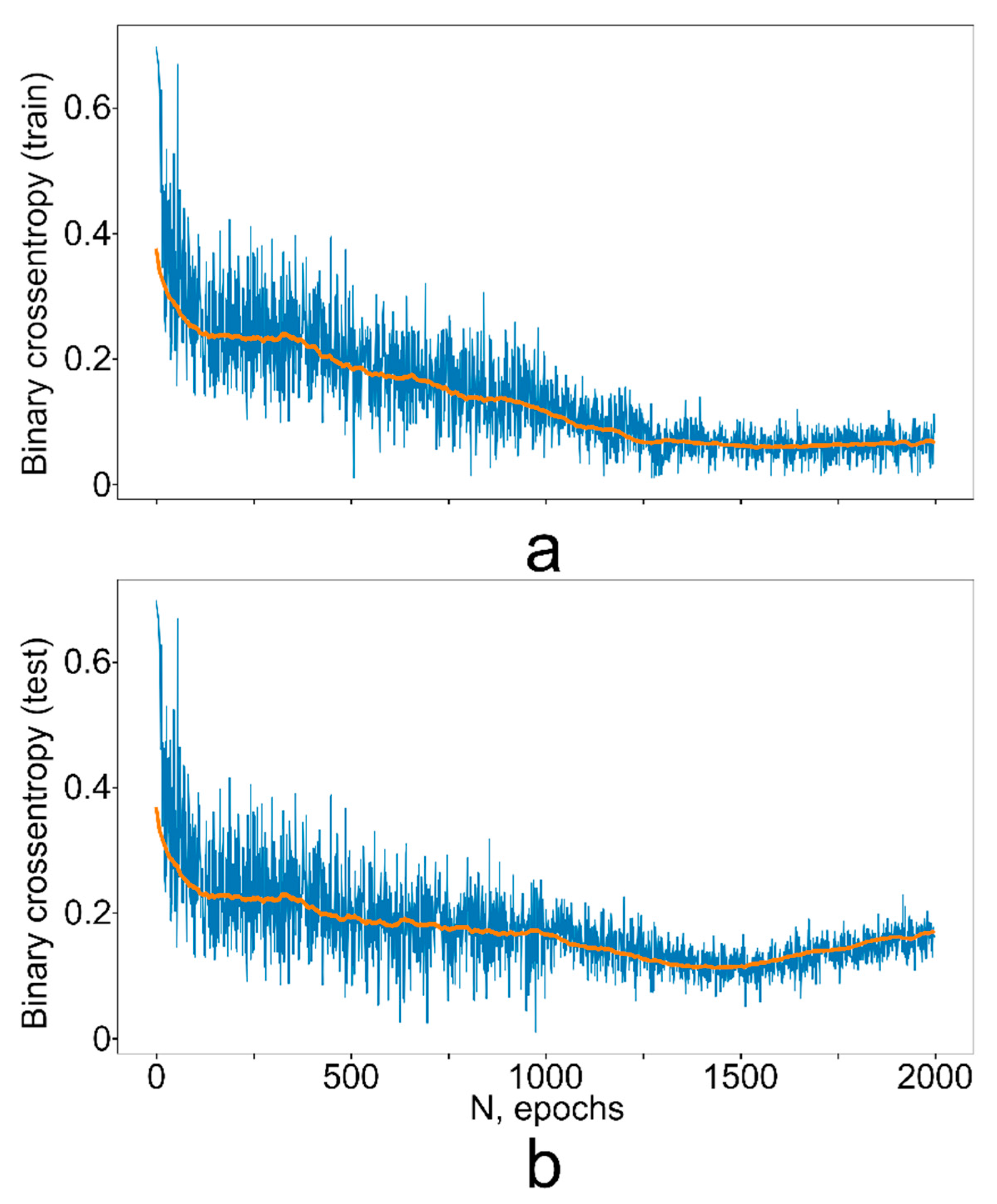
2.5. Neural Network Implementation and Tuning

The U-Net-like CNN described in Algorithm A1 was implemented in a Python-based (Python 3.7.3 was used) computational environment, which was built on top of the Keras framework [54] using Tensorflow [62] as a backend. All computations were performed on a PC with 1 GPGPU Nvidia Tesla K80 with 16 GB of RAM and required up to 10 h to train one CNN architecture.
We chose Adam [63] as an optimization algorithm to update the CNN weights and binary cross-entropy as a loss function. The latter is usually the method of choice when dealing with image segmentation and binary classification problems [64]. As stopping criteria for neural network training, we considered different approaches from setting the number of epochs to tracking for specific behaviors of the dynamically evaluated measures on the validation data. The latter approach is more progressive and allows the prevention of the CNN overfitting phenomenon (when the CNN performs significantly worse on the test data and better on the training data) by stopping the training process when performance metrics begin increasing for the training data and decreasing for the test data. In this case, the neural network starts to learn very specific patterns of the training dataset and loses the ability to generalize.
To tune the architecture of the neural network, we tested the following combinations of parameters (Algorithm A1, line #24), which correspond to different U-Net architectures: num_layers = {64, 32, 16}, depth = {2, 3, 4}, layer_rate = {2, 1.5, 1.2}, batch_norm = {True, False}, residual = {True, False}, dropout = {0, 0.5}. Thus, we performed a grid search over 216 different U-Net-like architectures and found several of the best ones which are suitable for forest damage segmentation.
All of the best results corresponded to the configuration when the number of layers was equal to 64, and dropout was applied. The best one, whereby an additional batch normalization is applied, corresponds to the following parameters: num_layers = 64, depth = 4, layer_rate = 2, batch_norm = True, residual = False, dropout = 0.5.
High-intensity fluctuations of the loss function shown in Figure 2, which corresponds to the best set of parameter values, are caused by the specificity of the algorithm used at the training stage. We did not have a prebuilt set of images to use for the training. We instead generated batches of training images randomly, on the fly, from source images presented in Table 1 (we randomly cropped source images to 256 × 256 resolution and applied augmentation), and we never showed exactly the same subset of images to the network. Therefore, there was only one step per epoch when training. All of that led to ambiguities in the objective function being minimized and likely caused the high values of variance. We also tried to change the default learning rate parameter for the Adam algorithm. Its decrease did not lead to a significant reduction of loss function fluctuations but increased the number of epochs required for network training. At the end of the learning process (after 1500 epochs), we obtained average values for the loss function that were less than 0.1.

2.6. Comparison to Traditional Machine Learning Algorithms
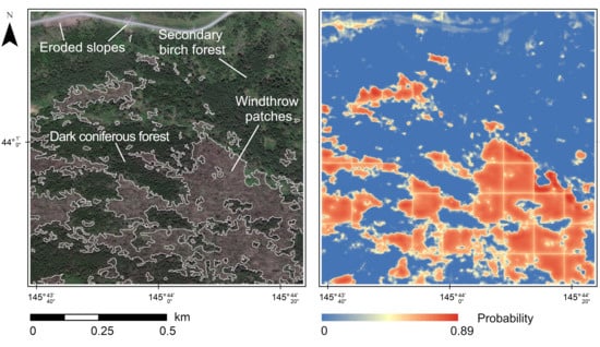
In contrast to CNNs, traditional machine learning methods do not account for neighboring pixels relative to the pixel being classified at a given moment. As we could expect, such methods should have lower performance than those that take into account values in neighboring pixels (i.e., use information about the correlation between pixels). For comparison purposes, we considered the following algorithms that have been widely used to solve various supervised learning problems: (1) naive Bayes classifier [65]; (2) logistic regression with L2 regularization [66]; (3) support vector machine [67]; 4) AdaBoost [68]. We used the default implementation of these algorithms as given in the sci-kit-learn package [69]. The naive Bayes classifier comes from the preposition that considered features are independent. It is relatively simple in training and usually yields to coarse classification results. However, it is fast and can handle large amounts of data. The logistic regression belongs to the class of generalized linear models. Being linear in its nature, it usually does not surpass more advanced methods based on the ensemble methodology (e.g., random forest, boosted trees). Due to its simplicity and possibility of probabilistic interpretation of the results, it is widely used in classification problems with continuous dependent variables, when it is possible to presume a quasi-linear relationship between those and the response probability. The support vector machine builds a hyperplane that maximizes a gap between classified subsets of points. Due to the kernel trick, it can handle not only linearly separable cases. It usually leads to good and reliable results. The latest one, the AdaBoost classifier, uses an ensemble of weak learners (e.g., decision trees) and tries to combine them into a weighted sum that represents a boosted classifier, which usually is much stronger and leads to good classification results. It is usually called, as one of the best out-of-the-box classifiers [70].
These methods were trained on a randomly chosen subset of 100,000 points from the original satellite images marked as “train” in Table 1. Validation was performed by applying trained algorithms to all pixels of satellite image #2. Further, we compared results with the best solution obtained by the U-Net-like CNN proposed above (Table 2).
Therefore, in comparison to traditional machine learning algorithms (e.g., logistic regression, decision trees, and SVM), the CNN-based approach takes into account the relationships between neighboring pixels and can recognize patterns that are specific for sites of disturbed forests. Another superiority of neural networks over traditional machine learning methods is that the latter can be used when only relatively small datasets are available. For example, it was quite hard to train the SVM algorithm on a dataset consisting of >1 M points due to the increasing computational complexity of the underlying optimization algorithm [71]. At the same time, the CNN-based approach can handle large quantities of data without problems.
The entire computational workflow is presented in Figure A1 in Appendix B.

3. Results

The method of recognizing windthrow patches based on pretrained U-Net-like CNN has an accuracy exceeding 94%. By contrast, the pixel-wise supervised learning methods, which are usually used to solve traditional classification problems (not related to image segmentation ones), do not allow us to achieve an accuracy higher than 85% (Table 2). It is worth noting that the accuracy values significantly depend on the type of terrain, which can look like a patch of damaged forest, e.g., have a similar color. If such a type of terrain is presented on the image, it can lead to decreased accuracy of the result obtained by traditional supervised learning methods. At the same time, the CNN-based approach turns out more robust in such cases; it can “understand” the pattern specific to the damaged forest and is not weakened by false-positive decisions. The MeanIoU values (Table 2) have the same monotonic behavior as the accuracy metrics do, but are being more sensitive and able to handle imbalanced cases, which lead to their drastic decreasing for traditional machine learning methods that usually show more false-positive cases.
The last layer of our CNN has “sigmoid” as an activation function. This allows us to interpret the output image (obtained on the forward path through the network) as the pixel-wise probability that a pixel belongs to a damaged forest patch. However, probabilities are not always the desired result. For the purpose of calculating the total area of damaged forest, it makes sense to choose a threshold value in order to convert probabilities to binary values. If the value of a probability exceeds this threshold, the pixel is classified as belonging to a windthrow site. The optimal threshold value can be estimated from the threshold-vs-accuracy curve by its optimization on a grid (Figure 3). In our study, we set the threshold from 0.4 to 0.45—which is close to the middle point of a typical range of probabilities (from 0 to 0.9) for an image.
It should be noted that the spatial borders of windthrow patches are not smooth and homogenous curves that bound a patch with 100% of fallen trees inside. Some trees in such patches can even be untouched, or there could be several partially damaged ones. As a result, these areas are highlighted with lesser intensity and have smaller probability values than those belonging to the central parts of windthrow patches (Figure 4 and Figure 5a).

4. Discussion

Our study shows that U-Net-like CNNs are able to identify small canopy gaps consisting of a few fallen trees and vice versa: if one or more trees survived inside windthrow, it is highlighted by smaller values of probability compared to those of a pure windthrow patch. CNN’s learn a pattern that is specific for a windthrow area. Therefore, we can expect that the higher the resolution of the source images, the more detailed the patterns that are included in the training dataset and the more accurate the obtained results of semantic segmentation. In particular, the use of higher-resolution images, for instance, LIDAR orthophotographs, provides data of greater detail than satellite imagery and leads to quite optimistic results [39]. As a prospective study, it would be interesting to perform a comparison analysis with images of different resolutions, for example, comparing Pleiades-1A/B imagery (resolution 0.5 m), WorldView-3 (resolution 0.31 m), and orthophotographs (resolution < 0.3 m). There are a number of problems related to forest utilization and management where images of 0.5 m can lead to quite satisfactory and acceptable results. However, there are still a lot of problems that require images of more detailed resolution. Among them are instance segmentation problems, e.g., tree counting problem, tree species detection, identification of small canopy gaps. On the other hand, the spatial extents at which unmanned aerial vehicles data are commonly acquired for vegetation mapping are generally limited to not more than a few hectares or square kilometers [47].
Hamdi et al. [39] pointed out that shadows of neighbor trees falling on windthrow patches prevent CNNs from correctly classifying such patches. Apparently, this is one of the important limitations associated with identifying the outfalls of individual trees and clarifying the boundaries of windthrow patches. If, in the case of unmanned aerial vehicles’ shadows, their related problems can be effectively minimized [72], then for satellite imagery, one should pay attention to the choice of images taking into account the angle of sunlight incidence. We can also assume that the dissected relief and presence of heavily shaded slopes of the northern exposures (in the northern hemisphere) and southern slopes (in the southern hemisphere) are factors significantly impacting the algorithm outputs as well the pixel-based methods of deciphering remote sensing data.
There are several limitations to using CNNs to obtain accurate segmentation of wind-disturbed forest areas. The territory chosen by us has high landscape diversity and contains objects that, in isolation, could be mistakenly classified as windthrows within a landscape context. For example, there are coastal areas that are similar in color and include eroded slopes with banded traces of erosion (similar to tree trunks) (Figure 4). These areas could be mistakenly classified as windthrows. Another source of such false-positive errors are seashores with logs thrown out after storms. However, artifacts of such kind can be easily removed by applying masks of vegetation cover or forested areas, which exclude false-positive decisions at the post-processing stage.
Another interesting case is caused by the visual similarity of windthrow patches and areas covered by deciduous tree species in a leafless state. We used early summer images (01 June 2015), when the growing season in Kunashir Islands was just beginning. Although deciduous tree species were already leafy at low altitudes, deciduous trees such as stone birch were leafless in the subalpine zone. For such areas, our neural network led to false-positive decisions (subalpine birch forests on Figure 5b) and near-zero precision value of identification windthrow patches. It should be noted that it is extremely hard or even impossible to correctly classify such leafless forest stands without using external data. The authors became able to correctly handle this case only due to information obtained by one of them during his fieldwork observations on Kunashir Island. We should note that at the beginning of the study, Figure 5b was mistakenly delineated as one including windthrow patches. In this regard, preparing training and validation data are very important steps and should be carried out very carefully, taking into account the time elapsed since the disturbance event took place and discrepancies in phenology, which could depend on local landscape conditions.

5. Conclusions

Our study shows possibilities for efficient use of U-Net-like CNNs in identifying windthrow patches in south boreal forests using satellite imagery of very high resolution. In contrast to pixel-wise methods of forest damage identification based on multi-spectral imagery, CNNs are demanding to the resolution of images used and able to understand patterns specific for windthrow areas. Since such patterns are hard to discover on satellite imagery of medium spatial resolution, it is unlikely that applying of deep learning methods, in particular U-Net-like CNN, to images of satellite systems like Sentinel-2 and Landsat will lead to results better than those, obtained by existing and well-known methods of pixel-wise object identification.
The CNN’s output is of a probabilistic nature and requires a threshold to be chosen to convert probabilities into a binary map. The choice of this threshold lies on the researcher’s shoulders. Our experience shows that a value of threshold approximately equal to 0.4–0.45 can yield quite good segmentation results. The average accuracy that can be reached by applying the U-Net-like CNN is 94%.
However, there are areas of terrain which have trunky-like patterns that are the source of false-positive decisions, when the forest without foliage is mistakenly classified as damaged. Such cases cannot be properly classified even by a human eye and require using additional information about forest tree composition and conditions of shooting.
There are important issues which concern the requirements imposed on training and validation images. Satellite imagery should be carefully selected taking into account (1) the time elapsed from the moment of the disturbance before the vegetation regeneration process has begun and (2) the possibility of shifts in tree phenology, e.g., caused by vertical temperature gradients in mountain landscapes, which result in incorrect classification of leafless forest stands as wind-disturbed areas since corresponding images are very similar in color and structure.
Our study shows that deep learning algorithms are reliable and efficient methods for a specific pattern segmentation based on very-high-resolution satellite imagery. Such methods become more popular due to the availability of high-performance computing facilities and satellite imagery of very-high-resolution. These are of high interest not only in view of damaged forest assessment but can be applied to various problems raising in forestry management and nature conservation. In this context, there are single object detection problems, in particular, tree positioning and tree species identification problems, which can be solved using a deep learning approach. Another interesting class of problems for deep learning is the detection of drying trees that is being subjected to external impacts, e.g., fungal infections or bark beetle outbreaks. These problems are of high interest in forestry and the case for further investigations for the appliance of deep learning approaches in vegetation science.

Supplementary Materials

The following are available online at https://www.mdpi.com/2072-4292/12/7/1145/s1, Figure S1: Satellite image of site #1; Figure S2: Satellite image of site #2; Figure S3: Satellite image of site #3; Figure S4: Satellite image of site #4; Figure S5: Satellite image of site #5; Figure S6: Satellite image of site #6; Figure S7: Satellite image of site #7; Figure S8: Satellite image of site #8; Figure S9: Satellite image of site #9; Figure S10: Satellite image of site #10.

Author Contributions

Conceptualization, D.E.K. and K.A.K.; methodology, D.E.K., software, D.E.K.; validation, D.E.K. and K.K; formal analysis, D.E.K.; investigation, D.E.K. and K.A.K.; resources, D.E.K.; data curation, K.D and K.A.K.; writing—original draft preparation, D.E.K. and K.A.; writing—review and editing, D.E.K. and K.A.K.; visualization, D.E.K. and K.A.K.; supervision, K.A.K.; project administration, K.A.K.; funding acquisition, K.A.K. All authors have read and agreed to the published version of the manuscript.

Funding

This research was funded by the Russian Science Foundation, grant number 18-74-00007.

Acknowledgments

We thank Viktoria Chilcote and Mark Chilcote for the manuscript proofreading. We are deeply grateful to the anonymous reviewers for for their constructive and valuable suggestions on the earlier drafts of this manuscript.

Conflicts of Interest

The authors declare no conflict of interest.

Appendix A

Algorithm A1: Recursive definition of U-Net-like CNN
1:DEF CONV_BLOCK(input, num_layers, batch_norm = False, residual= False, dropout = 0):
2:   x = Conv2D(num_layers, 3, activation = “relu”, padding= ‘same’)(input)
3:   x = BatchNormalization()(x) if batch_norm else x
4:   x = Dropout(dropout)(x) if dropout ! = 0 else x
5:   x = Conv2D(num_layers, 3, activation = “relu”, padding = ‘same’)(x)
6:   x = BatchNormalization()(x) if batch_norm is True else x
7:   output = Concatenate()([input, x]) if residual is True else x
8:   return output
9:DEF UNET_BLOCK(input, num_layers, depth, layer_rate = 2, batch_norm = False, residual = False, dropout = 0.5):
10:   if depth > 0:
11:    x = CONV_BLOCK(input, num_layers, batch_norm, residual, dropout)
12:    x = MaxPooling2D()(x)
13:    x = UNET_BLOCK(x, round(layer_rate * dim), depth − 1,
14:          layer_rate, batch_norm, residual, dropout)
15:    x = UpSampling2D()(x)
16:    x = Conv2D(dim, 2, activation = acti, padding = ‘same’)(x)
17:    x = Concatenate()([input, x])
18:    output = CONV_BLOCK(x, dim, batch_norm, residual)
19:   else:
20:    output = CONV_BLOCK(input, dim, batch_norm, residual, dropout)
21:  return output
22:DEF GET_UNet(input_shape, depth = 4, layer_rate = 2, batch_norm = False, residual = False, dropout = 0.5):
23:  input = Input(input_shape)
24:  x = UNET_BLOCK(input, num_layers = 64, depth = 4, layer_rate = 2, batch_norm = False, residual = False, dropout = 0.5)
25:  output = Conv2D(out_ch, 1, activation = ‘sigmoid’)(x)
26:  return Model(inputs = input, outputs = output)

Appendix B

Figure A1. Training and validation computational workflow.
Remotesensing 12 01145 g0a1

References

  1. Boose, E.R.; Foster, D.R.; Fluet, M. Hurricane impacts to tropical and temperate forest landscapes. Ecol. Monogr. 1994, 65, 369–400. [Google Scholar] [CrossRef]
  2. Everham, E.M.; Brokaw, N.V.L. Forest damage and recovery from catastrophic wind. Bot. Rev. 1996, 62, 113–185. [Google Scholar] [CrossRef]
  3. Ulanova, N.G. The effects of windthrow on forests at different spatial scales: A review. For. Ecol. Manag. 2000, 135, 155–167. [Google Scholar] [CrossRef]
  4. Fischer, A.; Marshall, P.; Camp, A. Disturbances in deciduous temperate forest ecosystems of the northern hemisphere: Their effects on both recent and future forest development. Biodiver. Conserv. 2013, 22, 1863–1893. [Google Scholar] [CrossRef]
  5. Mitchell, S.J. Wind as a natural disturbance agent in forests: A synthesis. Forestry 2013, 86, 147–157. [Google Scholar] [CrossRef] [Green Version]
  6. Webster, P.J.; Holland, G.J.; Curry, J.A.; Chang, H.R. Changes in tropical cyclone number, duration and intensity in a warming environment. Science 2005, 309, 1844–1846. [Google Scholar] [CrossRef] [Green Version]
  7. Turner, M.G. Disturbance and landscape dynamics in a changing world. Ecology 2010, 9, 2833–2849. [Google Scholar] [CrossRef] [Green Version]
  8. Altman, J.; Ukhvatkina, O.N.; Omelko, A.M.; Macek, M.; Plener, T.; Pejcha, V.; Cerny, T.; Petrik, P.; Strutek, M.; Song, J.-S.; et al. Poleward migration of the destructive effects of tropical cyclones during the 20th century. Proc. Natl. Acad. Sci. USA 2019, 115, 11543–11548. [Google Scholar] [CrossRef] [Green Version]
  9. Senf, C.; Seidl, R. Natural disturbances are spatially diverse but temporally synchronized across temperate forest landscapes in Europe. Glob. Chang. Biol. 2018, 24, 1201–1211. [Google Scholar] [CrossRef]
  10. Asbridge, E.; Lucas, R.; Rogers, K.; Accad, A. The extent of mangrove change and potential for recovery following severe Tropical Cyclone Yasi, Hinchinbrook Island, Queensland, Australia. Ecol. Evol. 2018, 8, 10416–10434. [Google Scholar] [CrossRef] [Green Version]
  11. Sommerfeld, A.; Senf, C.; Buma, B.; D’Amato, A.W.; Després, T.; Díaz–Hormazábal, I.; Fraver, S.; Frelich, L.E.; Gutiérrez, Á.G.; Hart, S.J.; et al. Patterns and drivers of recent disturbances across the temperate forest biome. Nat. Commun. 2018, 9, 4355. [Google Scholar] [CrossRef]
  12. Knohl, A.; Kolle, O.; Minayeva, T.Y.; Milyukova, I.M.; Vygodskaya, N.N.; Foken, T.; Schulze, E.-D. Carbon dioxide exchange of a Russian boreal forest after disturbance by wind throw. Glob. Chang. Biol. 2002, 8, 231–246. [Google Scholar] [CrossRef]
  13. Thürig, E.; Palosuo, T.; Bucher, J.; Kaufmann, E. The impact of windthrow on carbon sequestration in Switzerland: A model-based assessment. For. Ecol. Manag. 2005, 210, 337–350. [Google Scholar] [CrossRef]
  14. He, H.S.; Shang, B.Z.; Crow, T.R.; Gustafson, E.J.; Shifley, S.R. Simulating forest fuel and fire risk dynamics across landscapes—LANDIS fuel module design. Ecol. Model. 2004, 180, 135–151. [Google Scholar] [CrossRef]
  15. Bouget, C.; Duelli, P. The effects of windthrow on forest insect communities: A literature review. Biol. Conserv. 2004, 118, 281–299. [Google Scholar] [CrossRef]
  16. Lindenmayer, D.B.; Burton, P.J.; Franklin, J.F. Salvage Logging and Its Ecological Consequences, 2nd ed.; Island Press: Washington, DC, USA, 2012; 246p. [Google Scholar]
  17. Mokroš, M.; Výbošťok, J.; Merganič, J.; Hollaus, M.; Barton, I.; Koreň, M.; Tomaštík, J.; Čerňava, J. Early stage forest windthrow estimation based on unmanned aircraft system imagery. Forests 2017, 8, 306. [Google Scholar] [CrossRef] [Green Version]
  18. Global Forest Watch: Forest Monitoring Designed for Action. Available online: https://www.globalforestwatch.org (accessed on 28 February 2020).
  19. Hansen, M.C.; Potapov, P.V.; Moore, R.; Hancher, M.; Turubanova, S.A.; Tyukavina, A.; Thau, D.; Stehman, S.V.; Goetz, S.J.; Loveland, T.R. High-resolution global maps of 21st-century forest cover change. Science 2013, 6160, 850–853. [Google Scholar] [CrossRef] [PubMed] [Green Version]
  20. Potapov, P.; Hansen, M.C.; Kommareddy, I.; Kommareddy, A.; Turubanova, S.; Pickens, A.; Adusei, B.; Tyukavina, A.; Ying, Q. Landsat analysis ready data for global land cover and land cover change mapping. Remote Sens. 2020, 12, 426. [Google Scholar] [CrossRef] [Green Version]
  21. Chehata, N.; Orny, C.; Boukir, S.; Gyoon, D.; Wigneron, J.P. Object-based change detection in wind storm-damaged forest using high-resolution multispectral images. Int. J. Remote Sens. 2014, 35, 4758–4777. [Google Scholar] [CrossRef]
  22. Senf, C.; Seidl, R.; Pflugmacher, D.; Hostert, P.; Seidl, R. Using Landsat time series for characterizing forest disturbance dynamics in the coupled human and natural systems of Central Europe. ISPRS J. Photogram. 2017, 130, 453–463. [Google Scholar] [CrossRef]
  23. Haidu, I.; Fortuna, P.R.; Lebaut, S. Detection of old scattered windthrow using low cost resources. The case of Storm Xynthia in the Vosges Mountains, 28 February 2010. Open Geosci. 2019, 11, 492–504. [Google Scholar] [CrossRef]
  24. Rüetschi, M.; Small, D.; Waser, L.T. Rapid detection of windthrows using Sentinel-1 C-band SAR data. Remote Sens. 2019, 11, 115. [Google Scholar] [CrossRef] [Green Version]
  25. Einzmann, K.; Immitzer, M.; Böck, S.; Bauer, O.; Schmitt, A.; Atzberger, C. Windthrow detection in European forests with very high-resolution optical data. Forests 2017, 8, 21. [Google Scholar] [CrossRef] [Green Version]
  26. Jackson, R.G.; Foody, G.M.; Quine, C.P. Characterising windthrown gaps from fine spatial resolution remotely sensed data. For. Ecol. Manag. 2000, 135, 253–260. [Google Scholar] [CrossRef]
  27. Honkavaara, E.; Litkey, P.; Nurminen, K. Automatic storm damage detection in forests using high-altitude photogrammetric imagery. Remote Sens. 2013, 5, 1405–1424. [Google Scholar] [CrossRef] [Green Version]
  28. Duan, F.; Wan, Y.; Deng, L. A novel approach for coarse-to-fine windthrown tree extraction based on unmanned aerial vehicle images. Remote Sens. 2017, 9, 306. [Google Scholar] [CrossRef]
  29. Ravì, D.; Wong, C.; Deligianni, F.; Berthelot, M.; Andreu-Perez, J.; Lo, B.; Yang, G.-Z. Deep learning for health informatics. IEEE J. Biomed. Health 2017, 21, 4–21. [Google Scholar] [CrossRef] [Green Version]
  30. Christin, S.; Hervet, É.; Lecomte, N. Applications for deep learning in ecology. Methods Ecol. Evol. 2019, 10, 1632–1644. [Google Scholar] [CrossRef]
  31. Lamba, A.; Cassey, P.; Segaran, R.J.; Koh, L.P. Deep learning for environmental conservation. Curr. Biol. 2019, 29, R977–R982. [Google Scholar] [CrossRef]
  32. Long, J.; Shelhamer, E.; Darrell, T. Fully convolutional networks for semantic segmentation. arXiv 2015, arXiv:1411.4038v2. [Google Scholar]
  33. Arnab, A.; Torr, P.H.S. Pixelwise instance segmentation with a dynamically instantiated betwork. arXiv 2017, arXiv:1704.02386. [Google Scholar]
  34. LeCun, Y.; Bengio, Y.; Hinton, G. Deep learning. Nature 2015, 521, 436–444. [Google Scholar] [CrossRef]
  35. Krizhevsky, A.; Sutskever, I.; Hinton, G.E. Imagenet classification with deep convolutional neural networks. Commun. ACM 2017, 60, 84–90. [Google Scholar] [CrossRef]
  36. Shrestha, A.; Mahmood, A. Review of DL algorithms and architectures. IEEE Access 2019, 7, 53040–53065. [Google Scholar] [CrossRef]
  37. Brodrick, P.G.; Davies, A.B.; Asner, G.P. Uncovering ecological patterns with convolutional neural networks. Trends Ecol. Evol. 2019, 34, 734–745. [Google Scholar] [CrossRef]
  38. Kattenborn, T.; Eichel, J.; Fassnacht, F.E. Convolutional neural networks enable efficient, accurate and fine-grained segmentation of plant species and communities from high-resolution UAV imagery. Sci. Rep. 2019, 9, 17656. [Google Scholar] [CrossRef]
  39. Hamdi, Z.M.; Brandmeier, M.; Straub, C. Forest damage assessment using deep learning on high resolution remote sensing data. Remote Sens. 2019, 11, 1976. [Google Scholar] [CrossRef] [Green Version]
  40. Rammer, W.; Rupert, S. Harnessing deep learning in ecology: An example predicting bark beetle outbreaks. Front. Plant Sci. 2019, 10, 1327. [Google Scholar] [CrossRef]
  41. Wagner, F.H.; Sanchez, A.; Tarabalka, Y.; Lotte, R.G.; Ferreira, M.P.; Aidar, M.P.; Gloor, E.; Phillips, O.L.; Aragão, L.E.O.C. Using the U-Net convolutional network to map forest types and disturbance in the Atlantic rainforest with very high resolution images. Remote Sens. Ecol. Conserv. 2019, 5, 360–375. [Google Scholar] [CrossRef] [Green Version]
  42. Ronneberger, O.; Fischer, P.; Brox, T. U-Net: Convolutional networks for biomedical image segmentation. arXiv 2015, arXiv:1505.04597. [Google Scholar]
  43. Zhang, Z.; Liu, Q.; Wang, Y. Road extraction by deep residual U-Net. IEEE Geosci. Remote Sen. Lett. 2018, 15, 749–753. [Google Scholar] [CrossRef] [Green Version]
  44. Çiçek, Ö.; Abdulkadir, A.; Lienkamp, S.S.; Brox, T.; Ronneberger, O. 3D U-Net: Learning dense volumetric segmentation from sparse annotation. arXiv 2015, arXiv:1606.06650. [Google Scholar]
  45. Ayrey, E.; Hayes, D.J. The use of three-dimensional convolutional neural networks to interpret LiDAR for forest inventory. Remote Sens. 2018, 10, 649. [Google Scholar] [CrossRef] [Green Version]
  46. Mahdianpari, M.; Zhang, Y.; Salehi, B. Deep convolutional neural network for complex wetland classification using optical remote sensing imagery. IEEE J. Sel. Top. Appl. Earth Obs. Remote Sens. 2018, 11, 3030–3039. [Google Scholar] [CrossRef]
  47. Kattenborn, T.; Eichel, J.; Wiser, S.; Burrows, L.; Fassnacht, F.E.; Schmidtlein, S. Convolutional neural networks accurately predict cover fractions of plant species and communities in unmanned aerial vehicle imagery. Remote Sens. Ecol. Conserv. 2020. [Google Scholar] [CrossRef] [Green Version]
  48. Li, W.; Fu, H.; Yu, L.; Cracknell, A. Deep learning based oil palm tree detection and counting for high-resolution remote sensing images. Remote Sens. 2017, 9, 22. [Google Scholar] [CrossRef] [Green Version]
  49. Csillik, O.; Cherbini, J.; Johnson, R.; Lyons, L.; Kelly, M. Identification of citrus trees from unmanned aerial vehicle imagery using convolutional neural networks. Drones 2018, 2, 39. [Google Scholar] [CrossRef] [Green Version]
  50. Weather Archive in Yuzhno-Kurilsk. Available online: https://rp5.ru/Weather_archive_in_Yuzhno-Kurilsk (accessed on 24 March 2020).
  51. Pleiades-HR (High-Resolution Pptical Imaging Constellation of CNES). Available online: https://earth.esa.int/web/eoportal/satellite-missions/p/pleiades (accessed on 28 February 2020).
  52. WorldView-3 (WV-3). Available online: https://earth.esa.int/web/eoportal/satellite-missions/v-w-x-y-z/worldview-3 (accessed on 28 February 2020).
  53. Shorten, C.; Khoshgoftaar, T.J. A survey on image data augmentation for deep learning. J. Big Data 2019, 6, 60. [Google Scholar] [CrossRef]
  54. Chollet, F.; Fariz, R.; Taehoon, L.; de Marmiesse, G.; Oleg, Z.; Max, P.; Eder, S.; Thomas, M.; Xavier, S.; Frédéric, B.-C.; et al. Keras. GitHub. 2015. Available online: https://github.com/fchollet/keras (accessed on 26 March 2020).
  55. Gupta, S.; Girshick, R.; Arbelaez, P.; Malik, J. Learning rich features from RGB-D images for object detection and segmentation. arXiv 2014, arXiv:1407.5736v1. [Google Scholar]
  56. Chen, L.-C.; Papandreou, G.; Kokkinos, I.; Murphy, K.; Yuille, A.L. Deeplab: Semantic image segmentation with deep convolutional nets, atrous convolution, and fully connected CRFs. arXiv 2016, arXiv:1606.00915v2. [Google Scholar] [CrossRef]
  57. He, K.; Zhang, X.; Ren, S.; Sun, J. Deep residual learning for image recognition. In Proceedings of the IEEE Conference on Computer Vision and Pattern Recognition (CVPR), Las Vegas, NV, USA, 27–30 June 2016; pp. 770–778. [Google Scholar] [CrossRef] [Green Version]
  58. Yu, L.C.; Sung, W.K. Understanding geometry of encoder-decoder CNNs. arXiv 2019, arXiv:1901.07647v2. [Google Scholar]
  59. Ioffe, S.; Szegedy, C. Batch normalization: Accelerating deep network training by reducing internal covariate shift. arXiv 2015, arXiv:1502.03167v3. [Google Scholar]
  60. Srivastava, N.; Hinton, G.; Krizhevsky, A.; Sutskever, I.; Salakhutdinov, R. Dropout: A simple way to prevent neural networks from overfitting. J. Mach. Learn. Res. 2014, 15, 1929–1958. [Google Scholar]
  61. Evaluation of the CNN Design Choices Performance on ImageNet-2012. Available online: https://github.com/ducha-aiki/caffenet-benchmark (accessed on 24 March 2020).
  62. Abadi, M.; Agarwal, A.; Barham, P.; Brevdo, E.; Chen, Z.; Citro, C.; Corrado, G.S.; Davis, A.; Dean, J.; Devin, M.; et al. TensorFlow: Large-scale machine learning on heterogeneous systems. arXiv 2016, arXiv:1603.04467v2. [Google Scholar]
  63. Kingma, D.P.; Ba, J. Adam: A method for stochastic optimization. arXiv 2015, arXiv:1412.6980. [Google Scholar]
  64. Mannor, S.; Peleg, D.; Rubinstein, R. The cross entropy method for classification. In Proceedings of the 22nd International Conference on Machine Learning (ICML ’05); Association for Computing Machinery: New York, NY, USA, 2005; pp. 561–568. [Google Scholar] [CrossRef] [Green Version]
  65. Zhang, H. The optimality of naive Bayes. In Proceedings of the Seventeenth International Florida Artificial Intelligence Research Society Conference (FLAIRS), Miami Beach, FL, USA, 12–14 May 2004; Available online: https://www.aaai.org/Library/FLAIRS/2004/flairs04-097.php (accessed on 26 March 2020).
  66. Cramer, J.S. The origins of logistic regression. Tinbergen Inst. Work. Pap. 2002, 119, 16. [Google Scholar] [CrossRef] [Green Version]
  67. Cortes, C.; Vapnik, V. Support-vector networks. Mach. Learn. 1995, 20, 273–297. [Google Scholar] [CrossRef]
  68. Freund, Y.; Schapire, R. A decision-theoretic generalization of on-line learning and an application to boosting. J. Comput. Syst. Sci. 1997, 55, 119–139. [Google Scholar] [CrossRef] [Green Version]
  69. Pedregosa, F.; Varoquaux, G.; Gramfort, A.; Michel, V.; Thirion, B.; Grisel, O.; Blondel, M.; Prettenhofer, P.; Weiss, R.; Dubourg, V.; et al. Scikit-learn: Machine learning in Python. J. Mach. Learn. Res. 2011, 12, 2825–2830. [Google Scholar]
  70. Kégl, B. The return of AdaBoost.MH: Multi-class Hamming trees. arXiv 2013, arXiv:1312.6086. [Google Scholar]
  71. Moré, J.J. The Levenberg-Marquardt algorithm: Implementation and theory. In Numerical Analysis; Watson, G.A., Ed.; Springer: Berlin, Germany, 1978; pp. 105–116. [Google Scholar] [CrossRef] [Green Version]
  72. Lopatin, J.; Dolos, K.; Kattenborn, T.; Fassnacht, F.E. How canopy shadow affects invasive plant species classification in high spatial resolution remote sensing. Remote Sens. Ecol. Conserv. 2019, 5, 302–317. [Google Scholar] [CrossRef]
Figure 1. Kunashir Island and the study sites (see detailed description in Table 1).
Remotesensing 12 01145 g001
Figure 2. Loss function (blue) of the model for training (a) and testing (b) data with a rolling average (orange).
Remotesensing 12 01145 g002
Figure 3. Overall accuracy, the median value, and 25%–75% range are given.
Remotesensing 12 01145 g003
Figure 4. Source image of the study site #5 with corresponding mask (a) and windthrow segmentation performed by U-Net-like convolutional neural networks (b).
Remotesensing 12 01145 g004
Figure 5. Image of the study sites #6 (a) and #4 (b), source images (left), binary (middle), and continual (right) segmentation performed by U-Net-like convolutional neural networks.
Remotesensing 12 01145 g005
Table 1. Satellite imagery used for the study sites.
Site NumberSatelliteDateImage IDMain Vegetation TypesWindthrow PatchesUsing
1Pleiades-1A17 July 2015DS_PHR1A_201507170119408_FR1_PX_E146N44_0410_03088DC, M, SB +Train
2Pleiades-1A10 July 2015DS_PHR1A_201507100123116_FR1_PX_E145N44_1106_01880DB, DC, SB, +Validation
3Pleiades-1B01 June 2015DS_PHR1B_201506010122019_FR1_PX_E146N44_0109_03525DB, DC, SB, +Train
4WorldView-301 June 2015104001000CC65500DB, DC, SB, PTValidation
5Pleiades-1B01 June 2015DS_PHR1B_201506010122226_FR1_PX_E145N43_0822_01654DC+Train
6Pleiades-1B01 June 2015DS_PHR1B_201506010122226_FR1_PX_E145N43_0822_01654DC, DC-M+Validation
7Pleiades-1B01 June 2015DS_PHR1B_201506010122421_FR1_PX_E145N43_0619_02996DB, S, WTrain
8Pleiades-1B01 June 2015DS_PHR1B_201506010122226_FR1_PX_E145N43_0822_01654DB, DC-M, SB, W +Train
9Pleiades-1B01 June 2015DS_PHR1B_201506010122421_FR1_PX_E145N43_0619_02996DC, DC-M, W+Train
10Pleiades-1B01 June 2015DS_PHR1B_201506010122226_FR1_PX_E145N43_0822_01654S, WTrain
Abbreviations of vegetation types: DB—dwarf bamboo thickets, DC—dark conifer forests, DC-M—dark coniferous mixed forests, PT—dwarf pine thickets, S—seashore vegetation and sea areas, SB—stone birch forests, W—wetlands.
Table 2. U-Net-like CNN and pixel-wise supervised learning classifier comparison.
MethodAccuracy, %MeanIoU
Naive Bayes classifier56less 0.01
Logistic Regression + L2740.07
Support Vector Machine790.09
Boosted RF (AdaBoost)830.15
U-Net-like CNN940.46

