Generative Adversarial Networks Based on Collaborative Learning and Attention Mechanism for Hyperspectral Image Classification

Abstract

Classifying hyperspectral images (HSIs) with limited samples is a challenging issue. The generative adversarial network (GAN) is a promising technique to mitigate the small sample size problem. GAN can generate samples by the competition between a generator and a discriminator. However, it is difficult to generate high-quality samples for HSIs with complex spatial–spectral distribution, which may further degrade the performance of the discriminator. To address this problem, a symmetric convolutional GAN based on collaborative learning and attention mechanism (CA-GAN) is proposed. In CA-GAN, the generator and the discriminator not only compete but also collaborate. The shallow to deep features of real multiclass samples in the discriminator assist the sample generation in the generator. In the generator, a joint spatial–spectral hard attention module is devised by defining a dynamic activation function based on a multi-branch convolutional network. It impels the distribution of generated samples to approximate the distribution of real HSIs both in spectral and spatial dimensions, and it discards misleading and confounding information. In the discriminator, a convolutional LSTM layer is merged to extract spatial contextual features and capture long-term spectral dependencies simultaneously. Finally, the classification performance of the discriminator is improved by enforcing competitive and collaborative learning between the discriminator and generator. Experiments on HSI datasets show that CA-GAN obtains satisfactory classification results compared with advanced methods, especially when the number of training samples is limited.

1. Introduction

In the past few decades, hyperspectral data have become more convenient and inexpensive to acquire and collect [1]. The hyperspectral image (HSI) is a three-dimensional (3D) data cube, where each pixel has hundreds of spectral bands, and each spectral band corresponds to a 2D image. It combines abundant spectral information and spatial information simultaneously. HSI processing has been used for many practical applications, such as military [2], agriculture [3], and astronomy [4]. HSI classification is the foundation for these applications, which is achieved by assigning a specific class to each pixel. It mainly involves two tasks: effective feature representation and advanced classifier design.

For the traditional methods, the feature extraction and the classifier training are usually implemented separately. There are two alternative approaches to extract features: spectral-based feature extraction techniques and spatial–spectral feature extraction techniques. The former one focuses on transforming high-dimensional HSI data into a low-dimensional space, such as principal component analysis (PCA) [5], discriminative local metric learning [6], and sparse graph learning [7]. However, it is difficult to achieve accurate classification only by extracting spectral information from HSIs. Thus, joint spectral–spatial feature extraction techniques have become a new trend, such as morphological filtering [8,9], low-rank representation [10], superpixel-based methods [11,12], etc. Additionally, many representative classifiers have been proposed, such as sparse representation-based classification [13,14], decision trees [15], support vector machines (SVMs) [16,17,18], and random forests [19]. Among these classifiers, SVM aims at exploring the optimal separable hyperplane between different classes, which has shown robust performance in solving the small sample size and high-dimensional problems.

In the deep learning-based methods, feature extraction and classifier training can be realized synchronously. Compared with traditional methods, handcrafted features and specific domain knowledge are not necessary for deep learning-based methods. Many deep learning models have been utilized for HSI feature extraction and classification, such as stacked autoencoders (SAEs) [20,21,22,23], deep belief networks (DBNs) [24,25,26,27] and convolutional neural networks (CNNs) [28,29,30,31,32,33]. Chen et al. [20] designed a new SAE-based method by combining hierarchical feature extraction, PCA-based dimensionality reduction, and logistic regression classification to achieve HSI classification. Subsequently, various improvement methods of SAE, such as Laplacian SAE [21], segmented SAE [22], and compact and discriminative SAE [23] were proposed. In [24], the authors use a hybrid of PCA, DBN-based architecture, and logistic regression for HSI classification. Later, diversified DBN [25], feature fusion DBN [26], and spectral-adaptive segmented DBN [27] were proposed.

Different from SAE and DBN, CNN captures spatial dependencies by exploiting local connections and decreasing the number of parameters via sharing weights. In recent years, a series of CNN algorithms [28,29,30,31,32,33] have been developed for HSI classification. In [28], in order to extract spectral and spatial information, 1D-CNN and 2D-CNN are used individually. Then, these two kinds of features are concatenated to input the softmax layer for predicting the class labels. In [29], a 3D CNN (3DCNN) model was proposed to directly process the cubes of HSIs for spectral–spatial classification. Wu et al. [30] combined CNN and recurrent neural network (CRNN) to capture the spatial and spectral information. The deeper network model [31,32,33] is a new development direction of HSI classification. Song et al. [31] proposed a deep feature fusion network (DFFN) to extract the discriminative features of HSIs. It is implemented by utilizing the residual learning as the identity mapping and fusing the output of different layers. Lee et al. [32] constructed a deeper and wider network by using residual learning. It extracts spatial and spectral features by using a multi-scale convolutional filter bank. However, deeper CNNs easily lead to overfitting with limited training samples. To deal with this issue, Li et al. [34] designed a pixel-pair CNN model through re-organizing the limited training samples.

Generative adversarial networks (GANs) [35] are another new forefront to solve the small sample problem. GAN is constructed by combining a generator and a discriminator. The former focuses on generating samples that approximate the real samples, and the latter focuses on distinguishing whether the inputs are generated or real samples. GAN is trained via an adversarial procedure. By optimizing the discriminator and the generator alternately, GAN eventually gets a balance. In this case, the generator generates samples having the most similar distribution to real samples. At the same time, the discriminator achieves the best classification result. GANs have been successfully applied to text-to-image synthesis [36], future frame prediction [37], image-to-image translation [38], etc.

To improve the performance of GAN, many GAN-based methods mainly focus on developing various objective functions [39,40,41,42,43], generating high-quality samples [44,45,46], and improving training stability [47,48,49,50]. In the original GAN [35], Jensen–Shannon divergence is defined to estimate the similarity between the generated distribution and the real data distribution. It easily results in the vanishing gradient problem. In response to this problem, some metrics have emerged to improve the performance of GAN, such as Kullback Leibler divergence [39], least squares [40], Wasserstein distance [41,42], and absolute deviation [43]. To improve the quality of generated samples, the optimization of generated samples is achieved by removing the data outliers in [44]. Moreover, some works change the structure of the generator, such as the usage of an online-output model [45] and the construction of a Laplacian pyramid framework [46]. There is a lot of work on stabilizing the training process of GANs, such as the design of new network architectures [47] and the usage of heuristic tricks [48,49]. Radford et al. [47] constructed the GAN through using CNNs, in which pooling layers and fully connected layers are not used. Multi-discriminator GAN frameworks [48,49] are designed to provide stable gradients for the generator and further stabilize the adversarial training process of GANs. Additionally, there are some heuristic tricks to improve the training stability, such as feature matching, virtual batch normalization, and one-side label smoothing [50].

Recently, several researchers have tried to use GAN for HSI classification. GAN-based HSI classification methods focus on semi-supervised GANs [51,52,53,54,55,56,57] and spatial–spectral GANs [58,59]. In semi-supervised GAN methods, some methods were proposed by combining GAN with the traditional techniques, such as conditional random fields [51] and 3D bilateral filter [52]. Additionally, Zhan et al. [53] devised a semi-supervised 1D-GAN algorithm (HSGAN) for HSI classification. It uses unlabeled samples to train the discriminator and generator firstly, and then labeled samples are used to fine-tune the well-trained discriminator for classification. Later, improved HSGAN methods [54,55] were proposed by adding the majority voting or the dynamic neighborhood voting strategies for classification. Gao et al. [56] proposed a semi-supervised multi-discriminator GANs (MDGANs) to improve the judgment ability by averaging the results of multiple discriminators. In spatial–spectral GAN methods, Zhu et al. [57] proposed a 3D-GAN method to use both the spatial and spectral information of HSIs. 3D-GAN stabilizes the GAN training procedure by retaining only three principal components in HSIs, which causes 3D convolution to not actually slide among the spectral bands. Later, a multiclass spatial–spectral GAN method (MSGAN) was devised [58]. The discriminator of MSGAN is composed of a 1D and 2D convolutional structure to extract the spatial and spectral features of HSIs. Then, these extracted features are concatenated at the last fully connected layer of the discriminator to realize the spatial–spectral classification of HSIs.

These improved GAN methods promote the classification performance of HSIs by using unlabeled samples or extracting spatial–spectral features. However, these methods update the generator only according to the judgment from the discriminator. The guide information from the discriminator is limited, and the generator cannot directly access the real sample distribution. Thus, it is difficult to ensure that the generator is always updated toward real sample distribution. When the HSI data are involved, the generated samples are more difficult to approximate the real samples with complex spatial–spectral distribution, which may further degrade the classification performance of the discriminator.

In this paper, a novel symmetric convolutional GAN based on collaborative learning and attention mechanism (CA-GAN) is proposed for HSI classification. In CA-GAN, collaborative learning is devised to provide real sample information, which assists the sample generation in the generator. The collaborative learning is achieved by adding the shallow to deep features of real multiclass samples in the discriminator to the generator. Thus, the generator learns the distribution of real samples by collaborating and competing with the discriminator. In addition, a joint spatial–spectral hard attention module is incorporated into the generator, which is devised by using a dynamic activation function and an element-wise subtraction operation based on a multi-branch convolutional network. It can discard some misleading and confounding features of the generated samples and further improve the quality of generated samples. Moreover, a convolutional LSTM layer is merged into the discriminator to extract spatial features and capture long-term spectral dependencies among spectral bands. Finally, the well-trained discriminator of CA-GAN is adopted for HSI classification. The classification ability of the discriminator is promoted by using the high-quality generated samples. The innovation of this paper is summarized as follows.

(1) A symmetric convolutional GAN is optimized in an end-to-end manner to alleviate the over-fitting issue of HSI classification. In CA-GAN, the sample generation is guided not only by using the loss function from the discriminator but also by using the real sample information extracted from the discriminator. It prompts the generator to generate high-quality samples by using both collaborative and competitive learning.

(2) To learn complex spatial–spectral distribution of HSIs, joint spatial–spectral hard attention module emphasizes more discriminative features and suppresses less useful ones in the generation of both spatial and spectral dimensions. It guarantees the generated samples to approximate the real samples with spatial–spectral distribution.

(3) In CA-GAN, the discriminator captures global spectral dependencies instead of local correlation captured by the convolutional kernels in the existing GAN methods. The classification performance of CA-GAN is improved by extracting spatial–spectral features effectively and leveraging high-quality spatial–spectral generated samples.

The remainder of this paper is organized as follows. Section 2 briefly describes the background of GAN. The proposed CA-GAN method is expounded in Section 3. Subsequently, Section 4 exhibits the experimental results and analysis. Finally, some conclusions are drawn in Section 5.

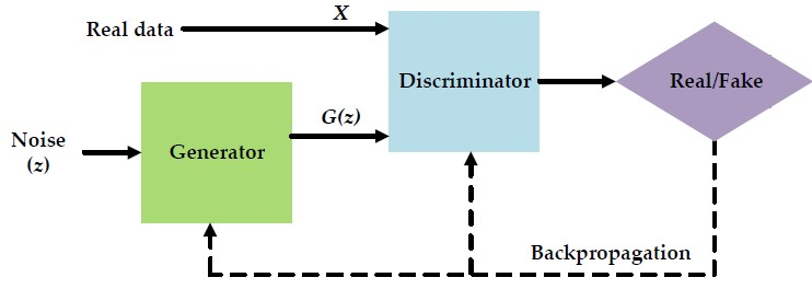
2. Generative Adversarial Networks

GAN is proposed by Goodfellow et al. [35], which uses a minimax game to train the generation model from the game theory perspective. Figure 1 shows the structure of GAN. It includes two networks; one is the generator $G$. The goal of $G$ is to transform the noise variable $z$ into the generated sample $G(z)$, which learns the distribution $p_{data}$ of real data $x$. The other is the discriminator $D$, whose goal is to distinguish whether a sample is real or generated. Both $G$ and $D$ implement non-linear mapping by using network structures, such as multi-layer perceptron.

In simple terms, $G$ wants to deceive $D$ and maximize the probability that $D$ makes a mistake by generating high-quality samples, and $D$ wants to make the best possible distinction between real samples $x$ and generated samples $G(z)$. The optimization of GAN is realized by finding the Nash equilibrium between $G$ and $D$. $G$ and $D$ are optimized by the value function $V(D,G)$:

$$\underset{G}{min}\underset{D}{max}V\left(D,G\right)=E_{x\sim p_{data}\left(x\right)}\left[logD\left(x\right)\right]+E_{z\sim p_z\left(z\right)}[log(1-D(G(z)))]$$

(1)

where $p_z(z)$ represents the distribution of the noise $z$. $E(·)$ represents the empirical estimation of the joint probability distribution. When the inputs are real samples $x$, the outputs of $D$ are indicated by $D(x)$. Similarly, the outputs $D(G(z))$ of $D$ correspond to the inputs from the generated samples $G(z)$.

In the process of network optimization, the generator $G$ and the discriminator $D$ are optimized in an alternating way. Specifically, given $G$, we optimize $D$ by maximizing $E_{x\sim p_{data}\left(x\right)}\left[logD\left(x\right)\right]+E_{z\sim p_z\left(z\right)}[log(1-D(G(z)))]$. Then, after arriving at a fixed $D$ value, $G$ is optimized by minimizing $E_{z\sim p_z\left(z\right)}[log(1-D(G(z)))]$. After many iterations, the entire network has reached an optimal balance. Through the competition of two networks, $D$ achieves the best evaluation results, and $G$ generates the data that learns the real distribution.

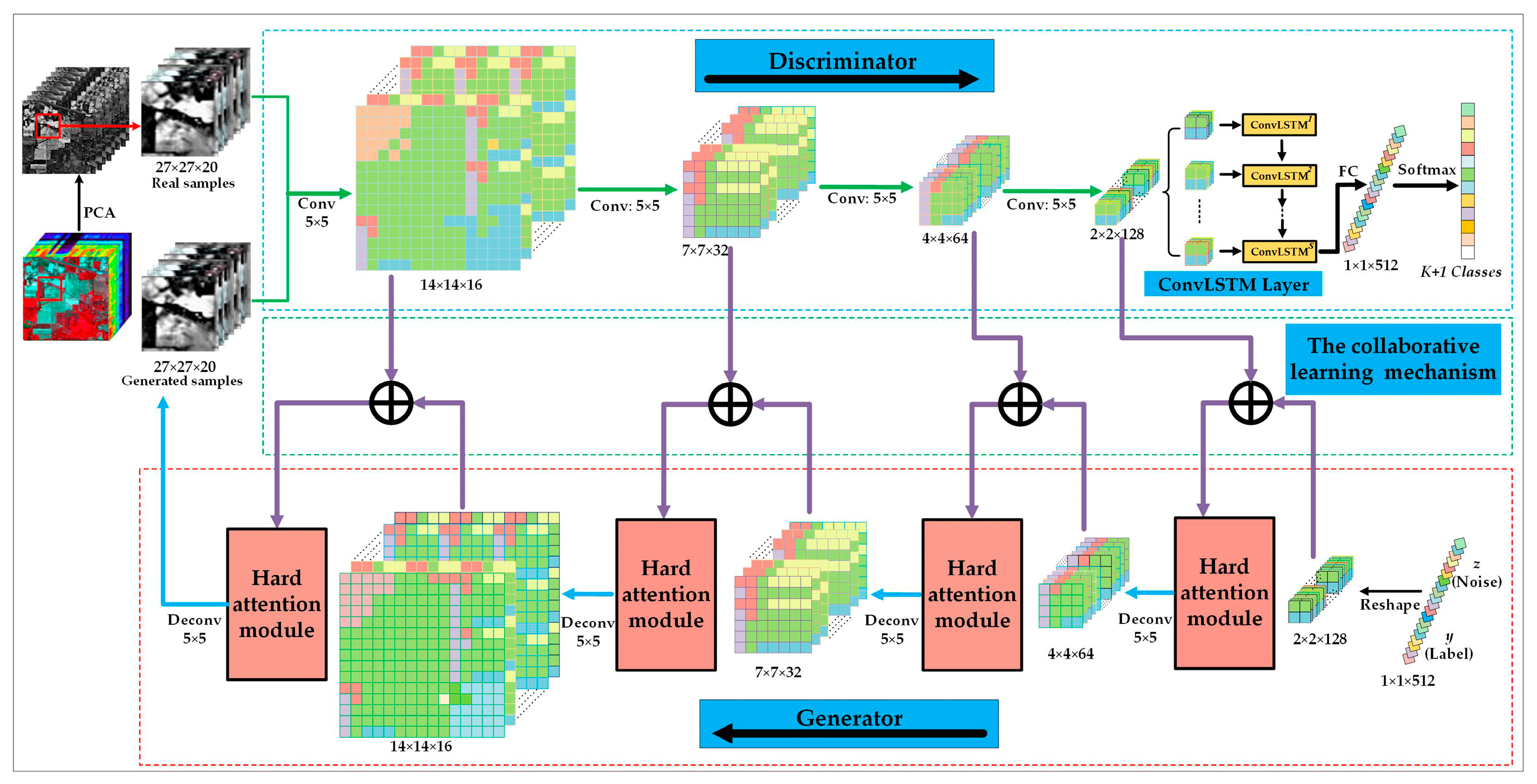
3. The Proposed CA-GAN Method

The structure of CA-GAN is based on a symmetric convolutional GAN. CA-GAN consists of three parts: the generator based on a joint spatial–spectral hard attention module, the discriminator based on convolutional LSTM, and the classification of CA-GAN based on collaborative and competitive learning. The conceptual framework of CA-GAN is shown in Figure 2. As shown in Figure 2, in the first part, the noise and the class labels are used as the input of the generator. Then, the transposed convolutional layer and joint spatial–spectral hard attention module are constructed to generate high-quality samples both in spatial and spectral dimensions. In the next part, the discriminator is constructed to capture joint spatial–spectral features by merging a convolutional long short-term memory (ConvLSTM) layer after the convolutional layer. In the final part, the collaborative learning mechanism is constructed based on the generator and discriminator with symmetrical structure. It impels the generator to generate high-quality samples by using the shallow to deep features of real samples extracted by the discriminator. The discriminator can collaborate with the generator to optimize the objective function of the generator. At the same time, the objective of the discriminator is to classify the generated samples as true classes, while the objective of the generator is to make the discriminator mistake. The classification performance of the discriminator is improved through competitive learning.

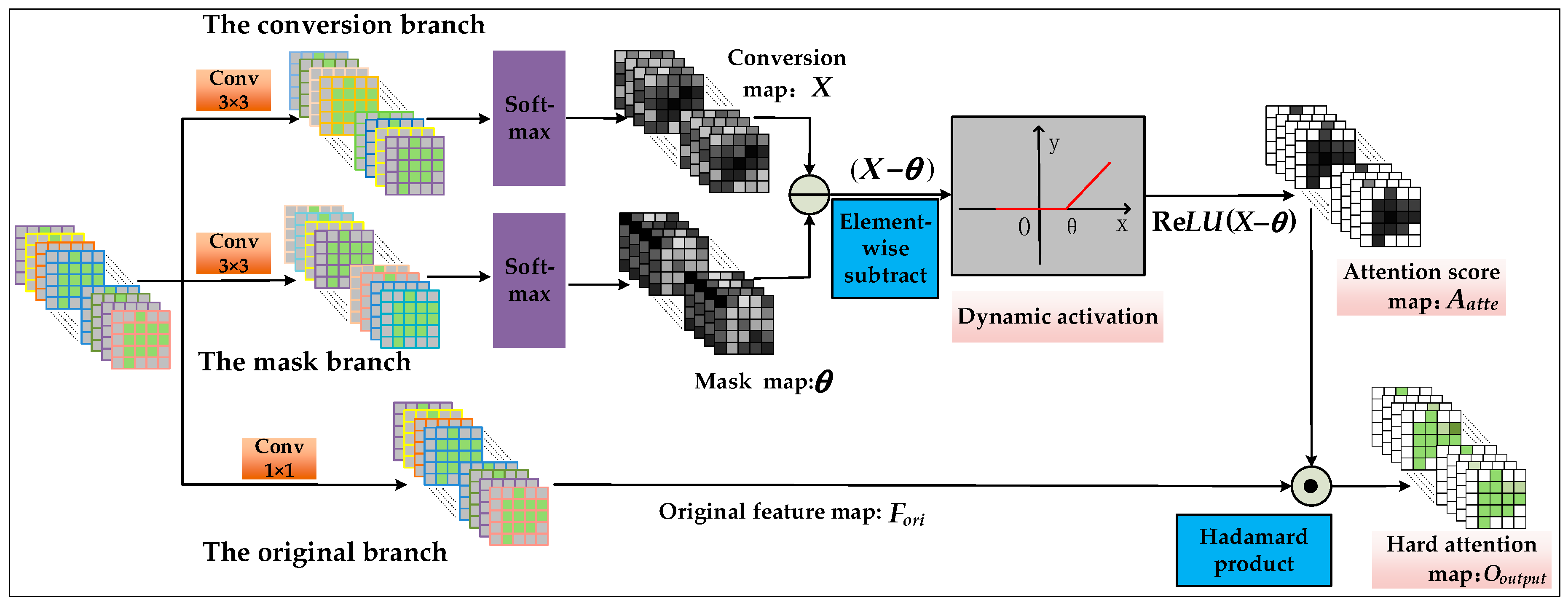
3.1. The Generator in CA-GAN Based on Joint Spatial–Spectral Hard Attention Module

In GAN, the classification performance of the discriminator is improved by utilizing the generated samples. Generating high-quality samples is pivotal for GAN-based HSI classification. However, it is difficult to approach the real HSI data in spectral and spatial domains because of high-dimensional spectral bands and various spatial distribution in HSIs. Radford et al. [47] suggested using transposed convolution and convolution without pooling layers and fully connected layers to construct the generator and discriminator in GAN. Most GAN-based HSI methods adopt this kind of architecture, such as HSGAN [53] and MSGAN [58]. In the generator, the transposed convolution operation can generate local spatial and spectral information of HSIs. However, it treats all the features equally during the generation process. Actually, some features facilitate the distribution of generated samples to approximate that of real samples, which further promotes the classification performance of the discriminator. On the contrary, some poor or noisy features hinder the generation of high-quality samples. Therefore, it is necessary to select appropriate spatial and spectral features in the process of sample generation.

In the generator of CA-GAN, the objective function of the generator is to maximize the probability that the discriminator classifies the generated samples as true classes. A new joint spatial–spectral hard attention module is devised in the generator to reserve meaningful features and suppress less useful ones along the spatial and spectral dimensions. It refines the features by using an adaptive spatial–spectral attention map. This attention map is calculated based on a multi-branch convolutional network by using a dynamic activation function and an element-wise subtraction operation. The spatial–spectral hard attention module is added before each transposed convolutional layer of the generator. It pays varied attention to spatial and spectral contextual features simultaneously. Finally, after adaptive feature selection, the features of the generated samples whose distribution is approximate to the real sample distribution are retained, and the confused and misleading ones are eliminated. The main structure of the joint spatial–spectral hard attention module is illustrated in Figure 3. It contains three branches: the conversion branch, the mask branch and the original branch. The spatial–spectral attention map is obtained by using element-wise subtract operation between the conversion and mask branches and mapping with the dynamic activation function. Then, features extracted from the original branch are refined by multiplying to the spatial–spectral attention map.

In HSIs, the training samples are 3D cubes and can be represented as $X_{train}=\left\{x_1,\cdot \cdot \cdot ,x_m,\cdot \cdot \cdot ,x_M\right\}$ in an $R^{n\times n\times d}$ feature space, where $M$ is the number of training samples, $n\times n$ indicates the size of the spatial neighborhood windows, and $d$ is the number of spectral bands. The labels of the training samples are denoted as $Y=\left\{y_1,\cdot \cdot \cdot ,y_m,\cdot \cdot \cdot ,y_M\right\}$, $y_m\in \left\{1, 2,\cdot \cdot \cdot ,K\right\}$, where $K$ is the number of classes. In the generator of CA-GAN, a random noise $z$, which follows the uniform distribution $\mu \left(-1,1\right)$, is used as the input. Moreover, the class label $y_m$ is also used as the input. After reshaping and transposing convolution operations on the input, the generated features are represented as $g\left(z,y\right)\in \left\{g^1\left(z,y\right),\cdot \cdot \cdot ,g^q\left(z,y\right),\cdot \cdot \cdot ,g^Q\left(z,y\right)\right\}$, where $1\le q\le Q$ and $q$ is the corresponding number of layers. These generated features are input to the joint spatial–spectral hard attention module.

In the joint spatial–spectral hard attention module, the converted map $X$ and the mask map $\theta$ are obtained by using the convolution and softmax layers in the conversion and mask branches, respectively. Here, the softmax layer normalizes the feature maps in the interval of $\left[0, 1\right]$. The converted map $X$ measures the effectiveness of features at different spatial and spectral locations in the original feature map. The mask map $\theta$ is the corresponding dynamic threshold, which can implement the feature elimination in the hard attention module. In the original branch, the convolutional layer uses $1\times 1$ kernels to obtain the original feature map $F_{ori}$. Then, an element-wise subtraction operation is implemented between the conversion map $X$ and mask map $\theta$. The different value $\left(X-\theta \right)$ is in the range of $\left[-1, 1\right]$. Subsequently, rectified linear unit (ReLU) is used to produce the spatial–spectral attention map $A_{\mathit{atte}}$ by mapping the difference value in the non-linear space. The activation function can be adjusted dynamically by the change of the threshold $\theta$. After the mapping, the spatial–spectral attention map $A_{\mathit{atte}}$ is constrained in the range of $[0,1]$. Finally, the output feature map $O_{output}$ of this attention module is acquired by performing the Hadamard product between the spatial–spectral attention map $A_{\mathit{atte}}$ and the original feature map $F_{\mathit{ori}}$. It can be formulated as follows:

$$\{\begin{array}{l}{O}_{output}=F_{ori}\odot \mathit{Re}LU\left(X-\theta \right)\\ F_{ori}=W_o\ast g\left(z,y\right)\\ X=soft\mathit{max}(W_c\ast g\left(z,y\right))\\ \theta =soft\mathit{max}(W_m\ast g\left(z,y\right))\end{array}$$

(2)

where ‘$\odot$’ indicates the Hadamard product, ‘$\ast$’ denotes the convolution operator, and $W_c$, $W_m$, and $W_o$ are the weight matrixes of the conversion branch, the mask branch, and the original branch, respectively.

The spatial–spectral attention map can pay various amounts of attention to different spatial and spectral features of the generated samples. When meaningful and discriminative features are generated, the output of the activation function is positive. In this case, the spatial–spectral attention map forces the conversion map $X$ to learn a larger score and the mask map $\theta$ to learn a smaller threshold. Thus, these meaningful and discriminative features are retained and emphasized in the generator. On the contrary, when confused and misleading features are generated, the spatial–spectral attention map makes the mask map $\theta$ learn a larger threshold. In this case, the value of $(X-\theta )$ is negative. After the activation function, the negative value becomes zero. Thus, these confused and misleading features can be eliminated in the generator. The dynamical activation function is formulated as follows.

$$\mathit{Re}LU\left(X-\theta \right)=\{\begin{array}{cc}X-\theta ,& \begin{array}{cc}if& \theta <X\end{array}\\ 0,& \begin{array}{cc}if& \theta \ge X\end{array}\end{array}$$

(3)

In CA-GAN, the generator has four transposed convolutional layers. Each transposed convolutional layer is constructed based on the convolutional kernel of $5\times 5$, and each transposed convolutional layer is followed by a batch normalization layer. Before each transposed convolutional layer, the joint spatial–spectral hard attention module is incorporated into the generator. The sizes of generated feature maps inputting to each attention module are $2\times 2\times 128,4\times 4\times 64,7\times 7\times 32,14\times 14\times 16$, respectively.

By analyzing the experiment, we found that embedding the joint spatial–spectral hard attention module in the generator has a better effect than embedding it in the discriminator. The reason may be that the discriminator easily outperforms the generator in most GANs. Therefore, embedding the joint spatial–spectral hard attention module in the discriminator has little effect on improving the classification ability of the discriminator, while embedding it in the generator will improve the generator significantly and assist the generator in generating high-quality samples.

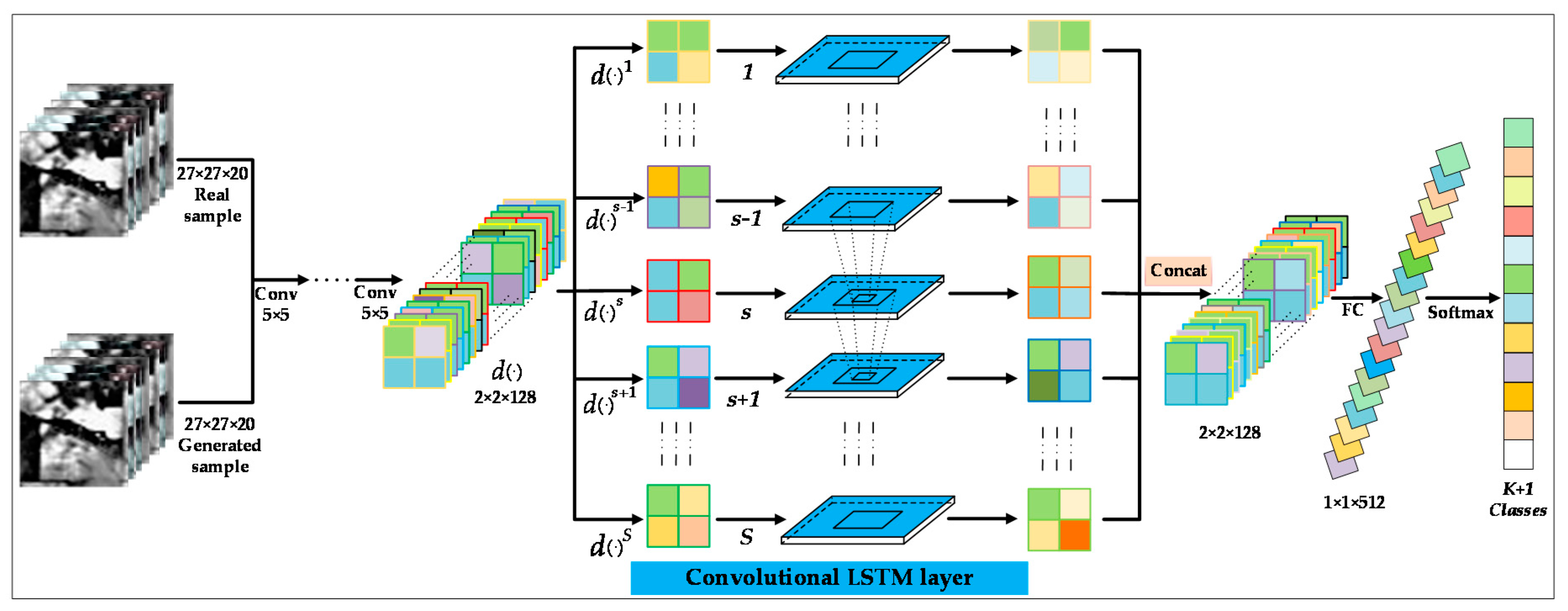
3.2. The Discriminator in CA-GAN Based on Convolutional LSTM for Joint Spatial–Spectral Feature Extraction

HSIs often include hundreds of spectral bands, which have provided valuable information to identify different land-cover classes. However, it is worth noting that the usage of only spectral information easily causes the degradation of classification performance, especially for the samples of the same class with different spectrums and the samples of different classes with similar spectrum. In the discriminator of CA-GAN, HSIs are considered as spatial–spectral sequences. The convolutional long short-term memory (ConvLSTM) [59] model is attempted to construct and extract joint spatial–spectral features for HSI classification. ConvLSTM is a modification of LSTM. LSTM can deal with the temporal sequence. The hyperspectral data are densely sampled from the visible to infrared spectrum. Since the spectral bands are approximately continuous, adjacent spectral bands have high correlation. Moreover, non-adjacent spectral bands may have long-term correlation. Thus, in ConvLSTM, the LSTM model is used to extract long-term spectral dependence in the spectral domain, and the convolution operator is incorporated into the LSTM network to extract spatial features across the spatial domain.

In CA-GAN, the input of the discriminator is the training sample $x_i$ and the generated sample $G(z,y_i)$. The main construction of the discriminator in CA-GAN is shown in Figure 4. In the discriminator, hierarchical features of input samples are extracted by four convolutional layers. $d(·)$ represents the features extracted by these convolutional layers, which is considered from the perspective of the spatial–spectral sequence. These features are input to ConvLSTM along the spectral channel sequentially. ConvLSTM captures the long-range dependencies among spectral bands by using the memory cell, and it extracts spatial information by using the convolution operator in the forget and input gates.

Specifically, features $d(·)$ are divided into several 3D cubes $(d{(·)}^1,\cdot \cdot \cdot ,d{(·)}^s,\cdot \cdot \cdot ,d{(·)}^s$ along the spectral channel, where $S$ is the number of cubes. $(d{(·)}^1,\cdot \cdot \cdot ,d{(·)}^s,\cdot \cdot \cdot ,d{(·)}^s$ is used to input to ConvLSTM in sequence. At the $s$-th moment, $d{(·)}^s$ is input to ConvLSTM. $c^{s-1}$ and $h^{s-1}$ represent the memory cell and hidden state of the $s-1$-th moment, respectively. The current memory cell $c^s$ is updated by calculating the input $d{(·)}^s$, the memory cell $c^{s-1}$, and the hidden state $h^{s-1}$ through the forget and input gates $f^s$ and $i^s$. The current hidden state $h^s$ is computed via the forget gate $f^s$, the input gate $i^s$, and the output gate $o^s$. Then, at the $s+1$-th moment, the output $o^{s+1}$ of the $s+1$-th moment is calculated by the hidden state $h^s$ of the previous moment and the input of the $s+1$-th moment $d{(·)}^{s+1}$. The memory cell $c^{s+1}$ and hidden state $h^{s+1}$ of the $s+1$-th moment are updated in the same way as that of the $s$-th moment. Finally, long-term spectral dependencies are extracted through the recursion of the previous cell to the next cell. At each moment, spatial information is extracted by the convolution operation of the input gate from the current moment and the forget gate from the previous hidden state. Thus, the spatial contextual correlation and long-term spectral dependencies of generated samples and real samples can be captured simultaneously in the discriminator of CA-GAN.

In the discriminator of CA-GAN, the input is the real samples and the generated samples with the same size of $27\times 27\times 20$. The discriminator extracts hierarchical features by using four convolutional layers with the convolutional kernel size of $5\times 5$. The sizes of the feature maps extracted by convolutional layers are $14\times 14\times 16,7\times 7\times 32,4\times 4\times 64,2\times 2\times 128$, respectively. Then, the ConvLSTM layer is merged after the convolutional layer to extract joint spatial–spectral information. In ConvLSTM, the padding operation is used during the convolution process, and the size of the convolutional kernel is $2\times 2$. Next, a fully connected layer is added after the ConvLSTM layer. Finally, the classification is implemented through a softmax layer in the discriminator. The softmax classifier predicts the class $y\in \left\{1,2,\cdot \cdot \cdot ,K,K+1\right\}$ of input samples. In this process, the objective function of the discriminator is to maximize the probability of classifying the real samples as true $K$ classes and the generated samples as the $K+1$-th class.

3.3. Classification of CA-GAN Based on Collaborative and Competitive Learning

In HSIs, the generation task is notoriously difficult due to the increasing data complexity, such as high dimension and complex spatial distribution. In GAN, the quality of the generated samples is not guaranteed, which may further degrade the classification performance of the discriminator. In addition, when the samples are generated by the generator, the generator itself has no way to evaluate the generated samples directly. GAN only uses the judgment of the discriminator to learn the distribution of real samples, which acts as a loss function to provide a learning signal to the generator. The generator is improved through the competition process between the generator and the discriminator. However, it is difficult to generate complex HSI data by only using the objective function. Moreover, the classification ability of the discriminator is easily superior to the generation ability of the generator. It indicates that there is information in the discriminator that the generator can use to assist sample generation. Inspired by this idea, CA-GAN uses additional information from the discriminator to assist sample generation in the generator.

In CA-GAN, a collaborative learning mechanism is devised between the generator and the discriminator, which is achieved by adding shallow and deep features of real multiclass samples in the discriminator to the generator. It is constructed by fusing each corresponding feature map of the same size in the generator and the discriminator. In the generator, the fused generated features are input to the next layer. This mechanism brings many advantages. It breaks the way of traditional optimization of only using competition between the generator and the discriminator. By utilizing additional information from the discriminator, the generator of CA-GAN can not only compete but also collaborate with the discriminator. Additionally, it alleviates the problem that the generator is optimized only by using the objective function from the discriminator. By utilizing the collaborative learning, the diversity of the generated samples can be improved. In this way, it is not easy to suffer from mode collapse.

The specific process of the collaborative learning mechanism is as follows. In the discriminator of CA-GAN, the generated samples and real samples are used as the input. The features extracted by four convolutional layers from real samples are represented as $d\left(x_i\right)=\left\{d^1\left(x_i\right),d^2\left(x_i\right),d^3\left(x_i\right),d^4\left(x_i\right)\right\}$. In the generator of CA-GAN, features generated by four transpose convolutional layers have the same sizes as the features extracted by four convolutional layers in the discriminator. By summing the features from real samples in the discriminator and the corresponding generated features of equal sizes in the generator, the new fused generated features $g^{\ast }\left(z,y_i\right)=\left\{g^{1^{\ast }}\left(z,y_i\right),g^{2^{\ast }}\left(z,y_i\right),g^{3^{\ast }}\left(z,y_i\right),g^{4^{\ast }}\left(z,y_i\right)\right\}$ are generated. These features are formulated as follows:

$$g^{u\ast }\left(z,y_i\right)=g^u\left(z,y_i\right)\oplus d^j\left(x_i\right)$$

(4)

where $d^j\left(x_i\right)$ represents the real sample features of the discriminator with the same size as the generated features $g^u\left(z,y_i\right)$, and ‘$\oplus$’ represents the element-wise summation operation.

In CA-GAN, the novel adversarial and collaborative objective functions of $G$ and $D$ are defined as follows:

$$\{\begin{array}{l}{l}_G={\displaystyle {\displaystyle \sum }_{i=1}^N}l\left(D\left(G\left(z,d^1\left(x_i\right),d^2\left(x_i\right),d^3\left(x_i\right),d^4\left(x_i\right),y_i\right),y_i\right)\right)\\ l_D={\displaystyle {\displaystyle \sum }_{i=1}^N}l(D\left(x_i\right),y_i)+{\displaystyle {\displaystyle \sum }_{i=1}^N}l\left(D\left(G\left(z,d^1\left(x_i\right),d^2\left(x_i\right),d^3\left(x_i\right),d^4\left(x_i\right),y_i\right),y_{K+1}\right)\right)\end{array}$$

(5)

where $l_D$ and $l_G$ represent the objective functions of the discriminator and the generator. $D(·)$ indicates the discriminator output, and $l(·)$ expresses the cross entropy.

As shown in Equation (5), for the real samples, the first term $\sum _{i=1}^{N}l\left(D(x_i\right),y_i)$ of $l_D$ indicates that the discriminator expects to have a high probabilities to their true classes. For the generated samples, $l_G$ and $l_D$ are not only adversarial, but also collaborative to each other. On the one hand, $l_G$ indicates that the generator expects the discriminator to classify the generated samples as true classes, while $l_D$ expects to classify these generated samples as $y_{K+1}$. On the other hand, the real sample features $\left\{d^1\left(x_i\right),d^2\left(x_i\right),d^3\left(x_i\right),d^4\left(x_i\right)\right\}$ from the discriminator are used to collaborate the sample generation in the generator. By using the collaborative learning, high-quality samples are generated. At the same time, the classification ability of the discriminator is facilitated by using competitive learning. Finally, after the generator and discriminator are updated by alternating optimization, the well-trained discriminator in CA-GAN is used for HSI classification.

3.4. The Procedure of CA-GAN

The proposed CA-GAN method combines a joint spatial–spectral hard attention module, convolutional LSTM, and collaborative learning mechanism into a unified optimization procedure. The detailed process of the designed CA-GAN method is described in

Table 1. The procedure of convolutional GAN based on collaborative learning and attention mechanism (CA-GAN) method.

INPUT: The training data $X_{train}=\left\{x_1,\cdot \cdot \cdot ,x_m,\cdot \cdot \cdot ,x_M\right\}$ and the test data $X_{test}=\{x_1^{test},x_2^{test},\cdot \cdot \cdot ,x_R^{test}\}$ from $K$ classes, the class labels of training samples $y\in \left\{y_1,\cdot \cdot \cdot ,y_k,\cdot \cdot \cdot ,y_K\right\}$, the mini-batch size $B$, the number of training epochs $E$ Begin Initialize: randomly initialize the parameters ${\theta }_d$ and ${\theta }_g$ of the discriminator and the generator For $E$ epochs do For $m$ training samples $\left\{x_1,x_2,\cdot \cdot \cdot ,x_m\right\}$ of every mini-batch   Generate $m$ noises $\left\{z_1,z_2,\cdot \cdot \cdot ,z_m\right\}$ from uniform distribution $\mu (-1,1)$   Concatenate noises with the class labels $\left\{y_1,y_2,\cdot \cdot \cdot ,y_m\right\}$   Input the training samples into the discriminator to obtain the real sample features $d(x_i)=\left\{d^1(x_i),d^2(x_i),d^3(x_i),d^4(x_i)\right\}$   Input noises $\left\{z_1,z_2,\cdot \cdot \cdot ,z_m\right\}$, class labels $\left\{y_1,y_2,\cdot \cdot \cdot ,y_m\right\}$, and real sample features $d(x_i)=\left\{d^1(x_i),d^2(x_i),d^3(x_i),d^4(x_i)\right\}$ to the generator $G$   Generate features $g(z,y)=\left\{g^1(z,y),\cdot \cdot \cdot ,g^q(z,y),\cdot \cdot \cdot ,g^Q(z,y)\right\}$   Obtain the fused generated features $g^{\ast }(z,y_i)=\left\{g^{1^{\ast }}(z,y_i),g^{2^{\ast }}(z,y_i),g^{3^{\ast }}(z,y_i),g^{4^{\ast }}(z,y_i)\right\}$ by using Equation (4)   Generate samples ${\left\{G(z,d^1(x_i),d^2(x_i),d^3(x_i),d^4(x_i),y_i)\right\}}_{i=1}^m$ by using the fused generated features Input generated samples and training samples to the discriminator Compute the objective function $l_D$ of the discriminator Update the parameters ${\theta }_g$ of the generator $G$ by minimizing $l_G$ $l_G={\displaystyle \sum _{i=1}^{N}l(D(G(z,d^1(x_i),d^2(x_i),d^3(x_i),d^4(x_i),y_i),y_i))}$ Update the parameters ${\theta }_d$ of the discriminator $D$ by minimizing $l_D$ $l_D={\displaystyle \sum _{i=1}^{N}l(D(x_i)},y_i)+{\displaystyle \sum _{i=1}^{N}l(D(G(z,d^1(x_i),d^2(x_i),d^3(x_i),d^4(x_i),y_i),y_{K+1}))}$ End for End for Classify the test data $X_{test}=\{x_1^{test},x_2^{test},\cdot \cdot \cdot ,x_R^{test}\}$ by the trained discriminator END OUTPUT: the labels of the test samples $X_{test}$

.

4. Experimental Results

In this part, three challenging hyperspectral datasets were adopted to verify the effectiveness of the proposed CA-GAN method. Some advanced HSI classification algorithms, radial based function (RBF)-SVM [17], SAE [20], DBN [24], pixel-pair features (PPF)-CNN [34], CRNN [30], HSGAN [53], and 3D-GAN [57] are used for comparison.

4.1. Data Description

The detailed description of three hyperspectral datasets is displayed as follows.

(1) Indian Pines: This scene was obtained in 1992 from Northwest Indiana. It contains $145\times 145$ pixels and 224 spectral bands. In this paper, 200 spectral bands are adopted for analysis. The Indian Pines dataset contains 16 vegetation classes. The false-color image (bands 50, 27, 17) and its ground truth are shown in Figure 5a and Figure 6a.

(2) Pavia University: Pavia University was captured in 2002 from northern Italy. It is composed of $610\times 340$ pixels and 115 spectral bands. It includes 9 classes. In this paper, 103 spectral bands are analyzed after removing 12 noise bands. Figure 5b and Figure 6b show the false-color composite image (bands 53, 31, 8) and the ground truth of this dataset.

(3) Washington: The Washington dataset was obtained at the Washington DC mall in 1995. It includes $750\times 307$ pixels, and the geometric resolution of each pixel is 2.8 m. In the experiments, 191 spectral bands are used for analysis. It includes 7 different categories. Figure 5c and Figure 6c show the false-color composite image (bands 70, 53, 50) of the Washington dataset and the ground truth.

4.2. Experimental Setting

To demonstrate the effectiveness of the CA-GAN algorithm, seven representative HSI classification methods are used for comparison, including RBF-SVM [16], SAE [20], DBN [24], PPF-CNN [34], CRNN [30], HSGAN [53], 3D-GAN [57]. In the experiment, the size of inputs will affect the classification performance. For fair comparison, all the comparison algorithms use their optimal parameters. For RBF-SVM, five-fold cross-validation is utilized to obtain the penalty and gamma parameters. In SAE, the radius of the spatial window is set as 7. For DBN, the spatial window of $5\times 5$ is used as the input to the network. For PPF-CNN, the value of the spatial window size is set according to the literature [34]. For CRNN, the batch size is set as 128, and other parameters are suggested in the literature [30]. For HSGAN, as suggested in [53], the convolutional kernel size is set as $1\times 3$ and $1\times 5$, and the number of training epochs is set as 200. For 3D-GAN, the spatial window of 3D input is set as $64\times 64\times 3$, and the convolutional kernel sizes are set according to the literature [57].

In CA-GAN, the main architecture and parameters are listed in

Table 2. The detailed and main structure of CA-GAN.

Network	No	Layer	Operation	Activation	Output Size
G	1	Hard Attention	$\{\begin{array}{l}conv:3\times 3\\ conv:3\times 3\\ conv:1\times 1\end{array}$	$\{\begin{array}{l}soft\mathit{max}\\ soft\mathit{max}\\ -\end{array}$	$2\times 2\times 128$
	2	Deconvolution	$5\times 5\times 64$	ReLU	$4\times 4\times 64$
	3	Hard Attention	$\{\begin{array}{l}conv:3\times 3\\ conv:3\times 3\\ conv:1\times 1\end{array}$	$\{\begin{array}{l}soft\mathit{max}\\ soft\mathit{max}\\ -\end{array}$	$4\times 4\times 64$
	4	Deconvolution	$5\times 5\times 32$	ReLU	$7\times 7\times 32$
	5	Hard Attention	$\{\begin{array}{l}conv:3\times 3\\ conv:3\times 3\\ conv:1\times 1\end{array}$	$\{\begin{array}{l}soft\mathit{max}\\ soft\mathit{max}\\ -\end{array}$	$7\times 7\times 32$
	6	Deconvolution	$5\times 5\times 16$	ReLU	$14\times 14\times 16$
	7	Hard Attention	$\{\begin{array}{l}conv:3\times 3\\ conv:3\times 3\\ conv:1\times 1\end{array}$	$\{\begin{array}{l}soft\mathit{max}\\ soft\mathit{max}\\ -\end{array}$	$14\times 14\times 16$
	8	Deconvolution	$5\times 5\times 20$	Tanh	$27\times 27\times 20$
D	1	Convolution	$5\times 5\times 16$	ReLU	$14\times 14\times 16$
	2	Convolution	$5\times 5\times 32$	ReLU	$7\times 7\times 32$
	3	Convolution	$5\times 5\times 64$	ReLU	$4\times 4\times 64$
	4	Convolution	$5\times 5\times 128$	Tanh	$2\times 2\times 128$
	5	ConvLSTM	$2\times 2\times 128$	Tanh/Sigmoid	$2\times 2\times 128$
	6	FC	-	-	$1\times 1\times 512$
	7	-	-	Softmax	$m\times (K+1)$ classes

. In Table 2, $G$ and $D$ represent the generator and the discriminator. As suggested in the literature [57], the dimension of input noise $z$ is $100\times 1\times 1$, and the number of training epochs is 600. By using a trial-and-error procedure, the learning rates of the discriminator and generator are 0.008 and 0.035. In the process of data acquisition, PCA is used to reduce the dimensionality and retain 20 principal components of HSIs. Then, each sample of reduced HSI data is represented by using a 27 × 27 spatial window centered on this sample. In this way, a 27 × 27 × 20 cube is extracted to represent each sample in HSIs.

In this paper, the overall accuracy (OA), average accuracy (AA), and Kappa coefficient (Kappa) are adopted to evaluate the classification performance of each algorithm. The final results are acquired by training 30 times independently. The experiments are based on the TensorFlow library on NVIDIA 2080Ti graphics card and are completed by Python language.

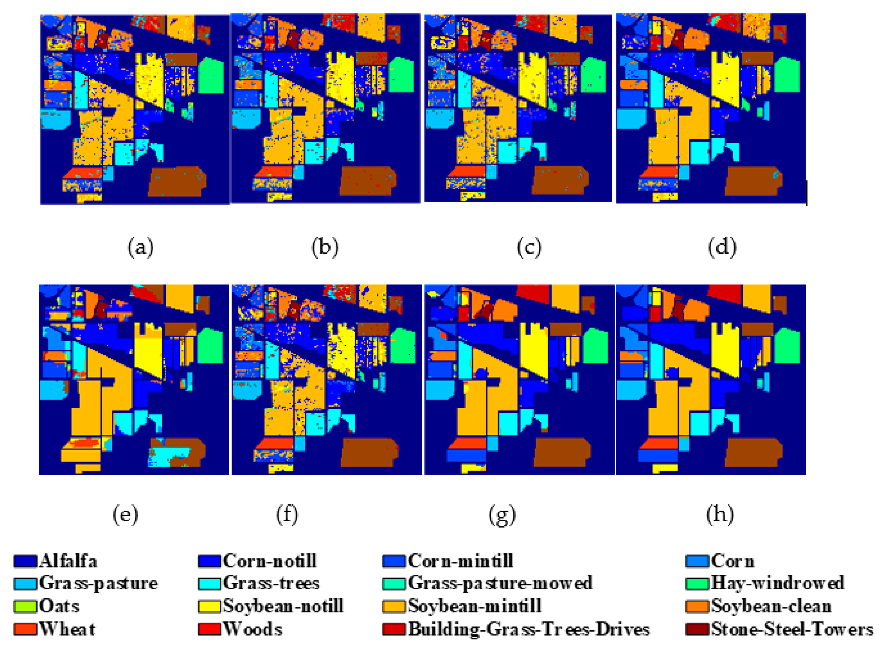
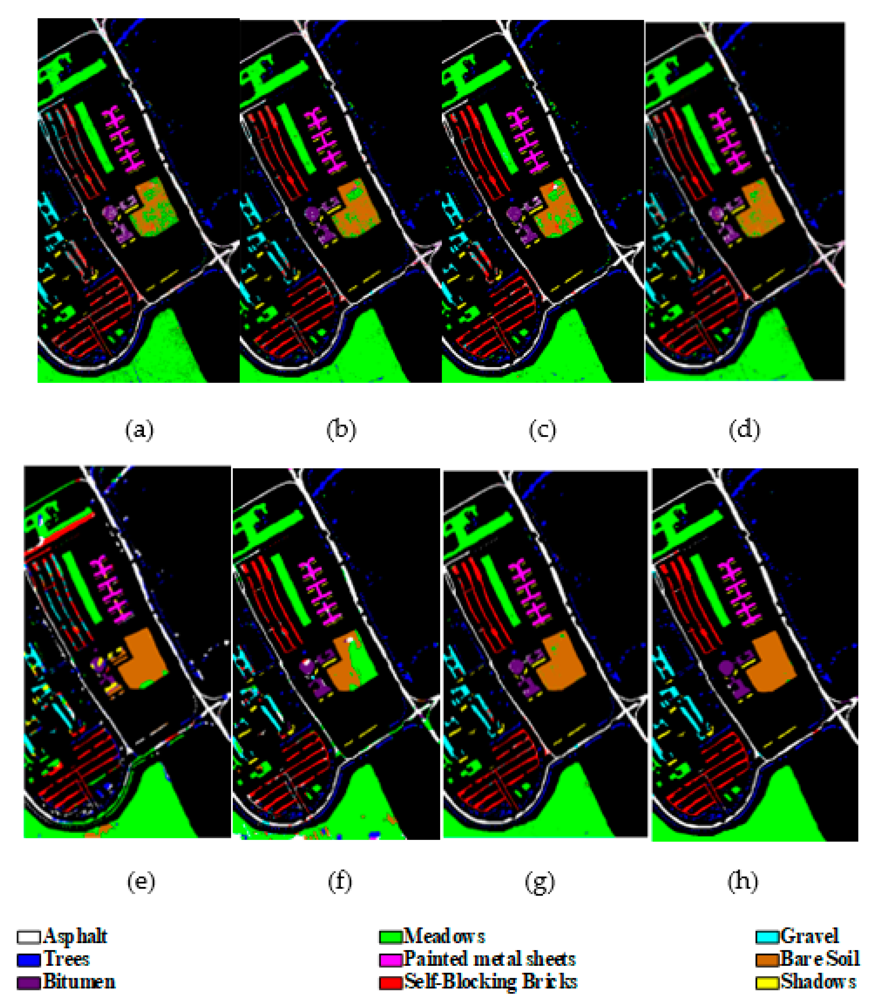
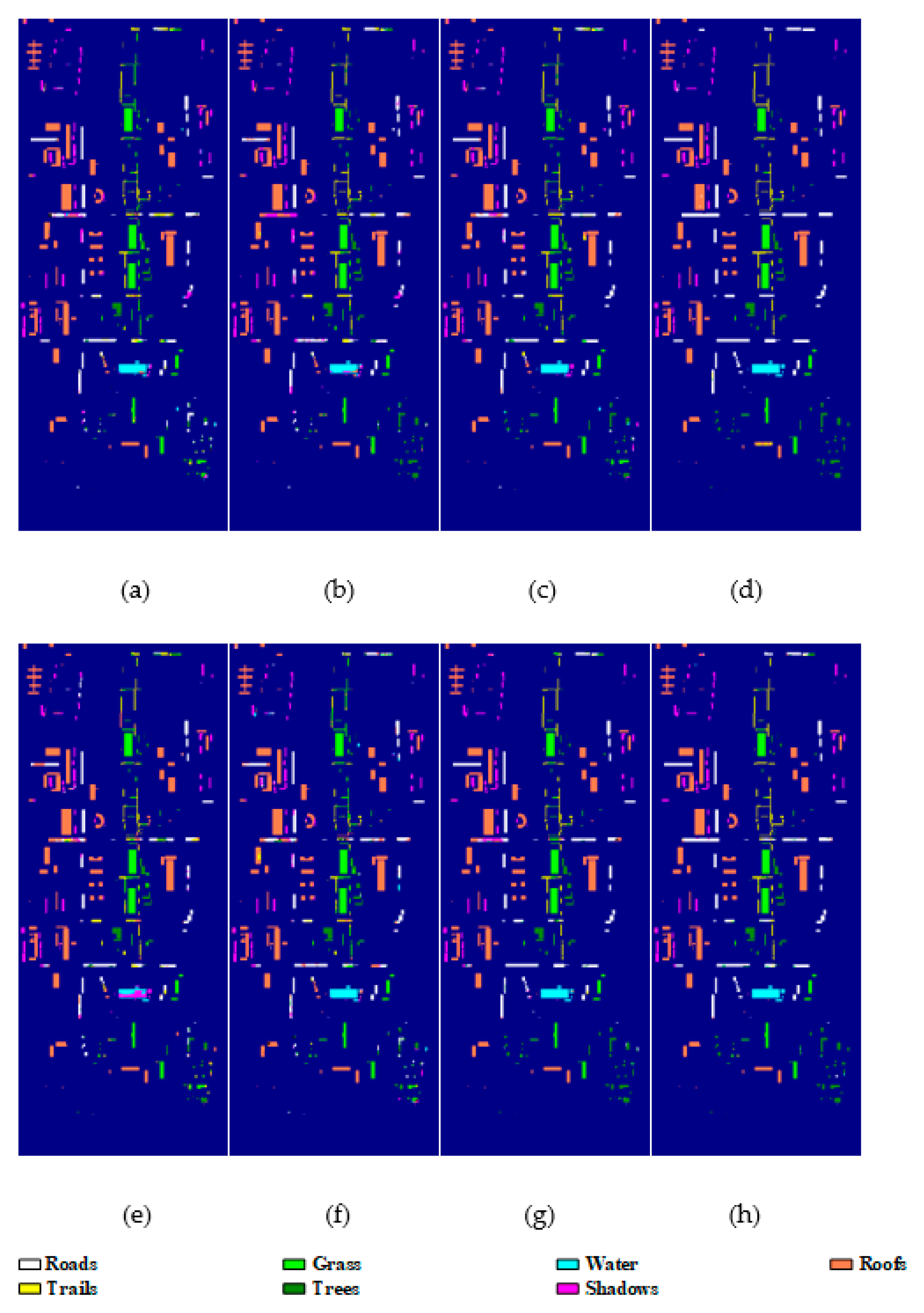
4.3. Experimental Results

(1) Classification results of the Indian Pines dataset: For the labeled samples, we randomly selected 5% from each class for training.

Table 3. Training and testing samples for each class of the Indian pines dataset.

Class		Number of Samples
No	Name	Training	Test	Total
1 2 3 4 5 6 7 8 9 10 11 12 13 14 15 16	Alfalfa Corn-notill Corn-mintill Corn Grass-pasture Grass-trees Grass-pasture-mowed Hay-windrowed Oats Soybean-notill Soybean-mintill Soybean-clean Wheat Woods Buildings-Grass-Trees-Drives Stone-Steel-Towers	2 71 42 12 24 36 1 24 1 49 123 30 10 63 19 5	42 1357 788 225 459 694 27 454 19 923 2332 563 195 1202 367 88	46 1428 830 237 483 730 28 478 20 972 2455 593 205 1265 386 93
Total		512	9737	10,249

lists the number of training and test samples in the experiment. The quantitative evaluations of various methods are displayed in

Table 4. Classification accuracies of various algorithms on the Indian Pines dataset.

Class	RBF-SVM	SAE	DBN	PPF-CNN	CRNN	HSGAN	3D-GAN	CA-GAN
1	6.1 ± 11.2	10.0 ± 6.4	13.6 ± 5.6	30.4 ± 8.4	81.8 ± 6.7	17.7 ± 5.2	90.9 ± 5.2	95.5 ± 4.5
2	72.9 ± 3.6	79.7 ± 2.3	79.8 ± 2.9	89.2 ± 2.1	91.5 ± 1.4	66.3 ± 1.1	91.0 ± 1.7	96.4 ± 2.1
3	68.0 ± 3.6	74.9 ± 4.8	70.5 ± 2.2	77.1 ± 2.7	91.8 ± 2.1	60.2 ± 2.9	90.4 ± 2.1	96.5 ± 2.3
4	59.0 ± 15.0	62.8 ± 8.3	71.3 ± 6.6	87.7 ± 3.7	86.3 ± 0.4	57.8 ± 4.7	93.7 ± 4.3	95.0 ± 4.7
5	87.0 ± 4.5	84.2 ± 3.3	80.1 ± 4.1	94.7 ± 1.0	94.1 ± 0.7	82.0 ± 6.1	93.2 ± 4.5	96.1 ± 4.0
6	92.4 ± 2.0	94.3 ± 1.7	94.2 ± 2.4	93.1 ± 1.9	95.2 ± 1.0	94.3 ± 2.2	95.4 ± 0.7	99.6 ± 0.4
7	0.0 ± 0.0	24.4 ± 18.8	28.1 ± 22.6	0.0 ± 0.0	64.1 ± 12.4	23.8 ± 12.2	94.9 ± 0.1	94.9 ± 0.1
8	98.1 ± 1.4	98.8 ± 0.4	98.5 ± 1.5	99.6 ± 0.3	100 ± 0.0	98.8 ± 0.3	99.9 ± 0.1	100 ± 0.0
9	0.0 ± 0.0	11.1 ± 10.1	9.5 ± 2.4	0.0 ± 0.0	33.1 ± 9.3	13.7 ± 12.1	53.5 ± 1.4	55.7 ± 9.8
10	65.8 ± 3.7	73.6 ± 3.8	73.2 ± 4.7	85.6 ± 2.8	87.6 ± 12.1	68.5 ± 3.6	94.2 ± 0.3	98.6 ± 0.3
11	85.3 ± 2.9	83.4 ± 2.0	82.7 ± 2.2	83.8 ± 1.6	98.4 ± 0.2	79.7 ± 0.5	94.7 ± 1.5	99.7 ± 0.2
12	69.6 ± 6.5	70.4 ± 8.0	62.0 ± 5.8	91.4 ± 3.1	84.7 ± 2.7	48.8 ± 4.5	92.1 ± 2.3	92.3 ± 3.4
13	92.3 ± 4.1	94.2 ± 4.3	95.7 ± 10.6	97.8 ± 0.9	78.7 ± 3.4	89.2 ± 2.7	95.5 ± 0.2	97.9 ± 1.6
14	96.6 ± 1.0	94.2 ± 1.5	94.4 ± 1.6	95.5 ± 1.1	92.5 ± 0.1	96.0 ± 1.1	95.6 ± 0.3	98.7 ± 0.4
15	41.7 ± 7.0	66.1 ± 5.6	64.2 ± 6.5	78.0 ± 2.4	83.1 ± 3.7	37.9 ± 11.4	87.7 ± 2.1	92.3 ± 1.0
16	75.2 ± 9.0	87.6 ± 8.1	80.5 ± 13.2	97.3 ± 1.3	94.3 ± 0.5	73.0 ± 5.3	92.6 ± 2.3	98.9 ± 1.1
OA (%)	77.8 ± 0.8	81.9 ± 0.1	80.6 ± 0.1	87.9 ± 0.8	93.0 ± 0.5	74.0 ± 0.9	93.5 ± 0.3	97.4 ± 0.5
AA (%)	61.3 ± 1.4	69.4 ± 1.9	68.3 ± 1.7	76.5 ± 0.6	92.1 ± 2.1	60.2 ± 2.6	84.8 ± 2.7	95.2 ± 2.2
Kappa (%)	74.5 ± 1.0	79.3 ± 1.1	77.8 ± 1.3	86.3 ± 0.9	92.9 ± 0.8	70.0 ± 1.0	93.1 ± 1.2	97.0 ± 0.6

. Table 4 includes the classification accuracies of different classes, and OA, AA, and Kappa for different methods. Among eight algorithms, the best accurate values are emphasized by marking with gray.

As shown in Table 4, deep learning-based methods are superior to RBF-SVM by extracting hierarchical non-linear features. PPF-CNN achieves better classification results than SAE and DBN by expanding the training samples. CRNN obtains better classification results than PPF-CNN by using recurrent neural network (RNN) to capture the spectral dependence of HSIs. Compared with HSGAN, 3D-GAN improves the classification performance because it fully use joint spatial–spectral information. Among these comparison methods, CA-GAN obtains the best classification performance in most classes by leveraging generated samples with high quality, especially in the classes having fewer samples. Additionally, among all the comparison methods, CA-GAN achieves the best classification accuracies in the OA, AA, and Kappa, which improve by at least 3.9%, 3.1% and 3.9%, respectively.

The classification visualization of various algorithms on the Indian Pines is shown in Figure 7. From Figure 7a,h we can see that RBF-SVM, SAE, DBN, PPF-CNN, and HSGAN have some visual noisy scattered points and misclassify many samples in the alfalfa, grass-pasture-mowed, oats, and buildings-grass-trees-drives classes. Compared with these methods, CRNN, 3D-GAN, and CA-GAN significantly reduce the noisy scattered points and effectively improve the regional uniformity. In comparison with other methods, CA-GAN has better regional uniformity in the wheat and corn-mintill classes, and it shows more accurate boundary of the grass-trees class.

(2) Classification results of the Pavia University dataset: We randomly selected 2% of the labeled data to train the network. The number of training and test samples is shown in

Table 5. Training and testing samples for each class of Pavia University.

Class		Number of Samples
No	Name	Training	Test	Total
1 2 3 4 5 6 7 8 9	Asphalt Meadows Gravel Trees Painted metal sheets Bare Soil Bitumen Self-Blocking Bricks Shadows	199 559 63 92 40 151 40 110 28	6233 17,531 1973 2880 1265 4727 1250 3462 891	6631 18,649 2099 3064 1345 5029 1330 3682 947
Total		1282	40,212	42,776

.

Table 6. Classification accuracies of various algorithms on the Pavia University dataset. OA: overall accuracy, AA: average accuracy.

Class	RBF-SVM	SAE	DBN	PPF-CNN	CRNN	HSGAN	3D-GAN	CA-GAN
1	89.1 ± 1.0	91.7 ± 0.3	90.6 ± 0.7	97.1 ± 0.8	90.2 ± 0.1	80.7 ± 38.3	88.9 ± 0.1	99.1 ± 0.2
2	95.3 ± 0.3	96.1 ± 0.7	96.9 ± 0.1	95.2 ± 0.7	99.0 ± 0.4	94.4 ± 1.5	99.8 ± 0.1	99.9 ± 0.1
3	61.6 ± 4.8	70.2 ± 1.5	68.4 ± 2.7	67.4 ± 6.8	87.4 ± 0.7	83.4 ± 4.6	89.6 ± 0.4	99.2 ± 0.2
4	89.1 ± 1.1	89.4 ± 1.4	89.7 ± 1.4	90.7 ± 6.8	88.7 ± 1.3	90.9 ± 1.9	94.8 ± 0.2	97.0 ± 2.3
5	96.2 ± 0.7	96.1 ± 0.7	96.0 ± 0.9	100.0 ± 0.0	90.7 ± 0.7	80.2 ± 10.1	99.8 ± 0.1	100 ± 0.0
6	77.0 ± 2.3	85.1 ± 0.9	84.0 ± 1.4	79.4 ± 2.8	96.5 ± 1.1	76.2 ± 3.3	99.8 ± 0.1	99.6 ± 0.3
7	73.9 ± 3.1	76.9 ± 2.3	74.1 ± 3.8	76.0 ± 7.2	83.1 ± 0.9	83.0 ± 2.0	96.1 ± 0.1	99.8 ± 0.2
8	84.5 ± 1.2	83.8 ± 0.9	84.0 ± 0.7	86.4 ± 3.9	84.2 ± 10.3	83.1 ± 3.9	88.4 ± 0.2	97.5 ± 0.3
9	98.5 ± 0.1	97.4 ± 0.7	98.0 ± 0.2	94.4 ± 1.7	67.8 ± 1.5	92.7 ± 2.4	90.8 ± 5.3	96.5 ± 1.7
OA (%)	88.5 ± 0.8	91.8 ± 0.1	90.2 ± 0.1	92.2 ± 0.7	95.4 ± 0.4	85.4 ± 2.4	97.0 ± 0.1	99.2 ± 0.6
AA (%)	85.6 ± 0.3	88.4 ± 0.6	89.1 ± 0.2	87.8 ± 0.9	83 ± 4.5	81.0 ± 1.0	92.1 ± 0.4	98.6 ± 1.2
Kappa (%)	86.1 ± 0.6	88.7 ± 0.3	88.9 ± 0.3	89.5 ± 0.9	92.5 ± 0.4	80.9 ± 3.2	96.0 ± 0.3	99.2 ± 0.7

shows the quantitative results of various methods. The most accurate results of the eight algorithms are marked by gray.

As shown in Table 6, PPF-CNN and CA-GAN have classified the painted metal sheet class completely correctly. The classification result of gravel and bitumen classes is significantly improved by CA-GAN. CA-GAN improves by at least 23.8% compared with PPF-CNN in the bitumen class. For the gravel class, CA-GAN improves by 37.6%, 29.0%, 30.8%, 31.8%, 11.8%, 15.8%, 9.6% compared with the other seven methods by using high-quality generated samples. The classification accuracies of CA-GAN for all the classes are over 96%. Moreover, CA-GAN exhibits the best classification performance in three evaluation indexes.

The classification visualization of various algorithms on the Pavia University is shown in Figure 8. As shown in Figure 8, the bare soil class is misclassified by RBF-SVM, SAE, DBN, PPF-CNN, and HSGAN. Compared with these methods, CA-GAN shows greater regional uniformity in this class. Many samples in the bitumen class have been misclassified due to the similar spectral signature with the asphalt class. CA-GAN improves the classification of these two classes. Compared with other seven algorithms, CA-GAN has better boundary integrity in the shadows class and better regional uniformity in the gravel and self-blocking bricks classes.

(3) Classification results of the Washington dataset: we randomly picked 3% of the labeled samples to train the CA-GAN. The number of training and test samples is listed in

Table 7. Training and testing samples for each class of the Washington dataset.

Class		Number of Samples
No	Name	Training	Test	Total
1 2 3 4 5 6 7	Roads Grass Water Roofs Trails Trees Shadows	86 51 19 31 38 35 168	2787 1663 611 1005 1240 1118 5443	2873 1714 630 1036 1278 1153 5611
	Total	428	13,867	14,295

.

Table 8. Classification accuracies of various algorithms on the Washington dataset.

Class	RBF-SVM	SAE	DBN	PPF-CNN	CRNN	HSGAN	3D-GAN	CA-GAN
1	94.1 ± 3.1	92.7 ± 1.8	94.2 ± 2.7	97.9 ± 0.6	92.2 ± 0.1	92.8 ± 3.1	96.1 ± 0.1	99.9 ± 0.1
2	93.4 ± 0.6	93.5 ± 0.1	92.6 ± 0.5	97.6 ± 0.1	93.5 ± 4.5	94.9 ± 0.1	95.4 ± 3.8	99.5 ± 0.3
3	98.3 ± 0.1	92.7 ± 0.5	91.5 ± 0.8	100.0 ± 0.0	86.6 ± 0.1	95.8 ± 0.3	99.6 ± 0.0	100 ± 0.0
4	88.2 ± 3.9	90.1 ± 2.4	92.9 ± 3.4	95.6 ± 3.1	93.8 ± 2.4	90.8 ± 3.5	99.0 ± 1.1	98.8 ± 2.1
5	95.6 ± 0.4	99.0 ± 0.6	98.9 ± 1.1	99.9 ± 0.1	96.9 ± 0.3	90.0 ± 0.0	99.5 ± 0.3	99.9 ± 0.1
6	91.6 ± 3.5	92.8 ± 1.6	91.1 ± 1.8	97.5 ± 1.2	91.5 ± 4.7	91.6 ± 1.1	97.0 ± 1.0	99.2 ± 0.5
7	98.2 ± 1.5	93.2 ± 0.5	93.5 ± 0.3	94.9 ± 0.1	99.3 ± 0.3	94.7 ± 1.3	98.2 ± 0.7	99.6 ± 0.1
OA (%)	93.7 ± 0.4	94.6 ± 0.4	94.1 ± 0.9	95.7 ± 0.3	95.9 ± 0.4	92.5 ± 1.6	97.2 ± 0.3	99.5 ± 0.5
AA (%)	92.3 ± 0.8	94.2 ± 0.6	94.6 ± 1.0	95.9 ± 0.5	94.7 ± 0.1	90.8 ± 1.8	97.0 ± 0.5	98.9 ± 0.7
Kappa (%)	93.7 ± 0.6	94.2 ± 0.5	93.9 ± 1.1	95.5 ± 0.3	94.7 ± 0.3	90.3 ± 1.6	96.7 ± 0.4	99.2 ± 0.4

shows the quantitative results of various methods. From Table 8, RBF-SVM misclassifies many samples in the roofs class, and CRNN misclassifies many samples in the water class. Compared with RBF-SVM, CA-GAN improves by 10.6% for the roofs class. Compared with CRNN, CA-GAN improves by 13.4% for the water class. Compared with other seven methods, CA-GAN obtains the highest OA, AA, and Kappa values. It improves by 5.8%, 4.9%, 5.4%, 3.8%, 3.6%, 7.0%, and 2.3% compared with the other seven methods in the OA index.

Figure 9 shows the classification visualization of various algorithms on the Washington dataset. From Figure 9, we can see that DBN and CRNN misclassify the water and shadows classes. The proposed CA-GAN method achieves better classification performance for these two classes. For the roads class, all the RBF-SVM, SAE, DBN, CRNN, HSGAN, and 3D-GAN methods have different degrees of misclassification. In contrast to these methods, PPF-CNN and CA-GAN show better regional uniformity in the roads class. Compared with PPF-CNN, CA-GAN performs better regional uniformity in the roofs class. In addition, compared with other seven methods, CA-GAN shows better boundary integrity in the trees class.

4.4. Analysis on Running Time

Table 9. Running time of different methods on the Indian Pines dataset.

Dataset	Method	Training Time (s)	Test Time (s)
Indian Pines	RBF-SVM	0.4 ± 0.1	1.2 ± 0.1
	SAE	76.3 ± 8.4	0.2 ± 0.1
	DBN	114.3 ± 20.1	0.2 ± 0.1
	PPF-CNN	2056.0 ± 36.7	5.3 ± 0.3
	CRNN	2184.5 ± 75.7	49.9 ± 12.3
	HSGAN	444.7 ± 73.1	0.3 ± 0.0
	3D-GAN	597.67 ± 60.8	0.3 ± 0.0
	CA-GAN	712.9 ± 3.1	0.3 ± 0.1

,

Table 10. Running time of different methods on the Pavia University dataset.

Dataset	Method	Training Time (s)	Test Time (s)
Pavia University	RBF-SVM	0.5 ± 0.1	1.4 ± 0.2
	SAE	12.9 ± 0.9	0.5 ± 0.0
	DBN	27.4 ± 0.9	0.5 ± 0.0
	PPF-CNN	2414.0 ± 374.0	19.8 ± 6.2
	CRNN	2717.6 ± 54.6	127.2 ± 4.3
	HSGAN	580.2 ± 20.5	0.5 ± 0.1
	3D-GAN	724.4 ± 50.7	0.6 ± 0.1
	CA-GAN	949.9 ± 80.2	0.6 ± 0.1

and

Table 11. Running time of different methods on the Washington dataset.

Dataset	Method	Training Time (s)	Test Time (s)
Washington	RBF-SVM	0.3 ± 0.0	0.2 ± 0.0
	SAE	28.9 ± 0.4	0.2 ± 0.0
	DBN	29.2 ± 0.1	0.2 ± 0.0
	PPF-CNN	926.8 ± 29.5	5.2 ± 0.5
	CRNN	1328.1 ± 56.9	64.8 ± 12.3
	HSGAN	493.4 ± 73.8	0.2 ± 0.1
	3D-GAN	673.3 ± 23.7	0.3 ± 0.1
	CA-GAN	814.2 ± 7.2	0.3 ± 0.1

show the training and test time of various methods on three datasets. From Table 9, Table 10 and Table 11, RBF-SVM and DBN consume less time than the other methods in the training procedure due to the 1D input. HSGAN, 3D-GAN, and CA-GAN require less training time to optimize the network than PPF-CNN and CRNN, and they take longer than the other methods. This is because GAN needs lots of time to optimize the generator and discriminator alternately. Compared with HSGAN and 3D-GAN, CA-GAN spends longer time due to the increasing parameters of the attention module and convLSTM. Among all the methods, PPF-CNN and CRNN are the most time-consuming in terms of the training time. The computing time of PPF-CNN is mainly consumed in the augmentation of training samples, especially for numerous training samples. CRNN is time-consuming due to the recurrent neural network. In the testing procedure, PPF-CNN and CRNN cost more time because PPF-CNN adopts the voting strategy with the surrounding samples and CRNN adopts a complex recurrent network. CA-GAN takes similar time as 3D-GAN and convLSTM. It costs 0.3 s, 0.6 s, and 0.3 s on three datasets, respectively.

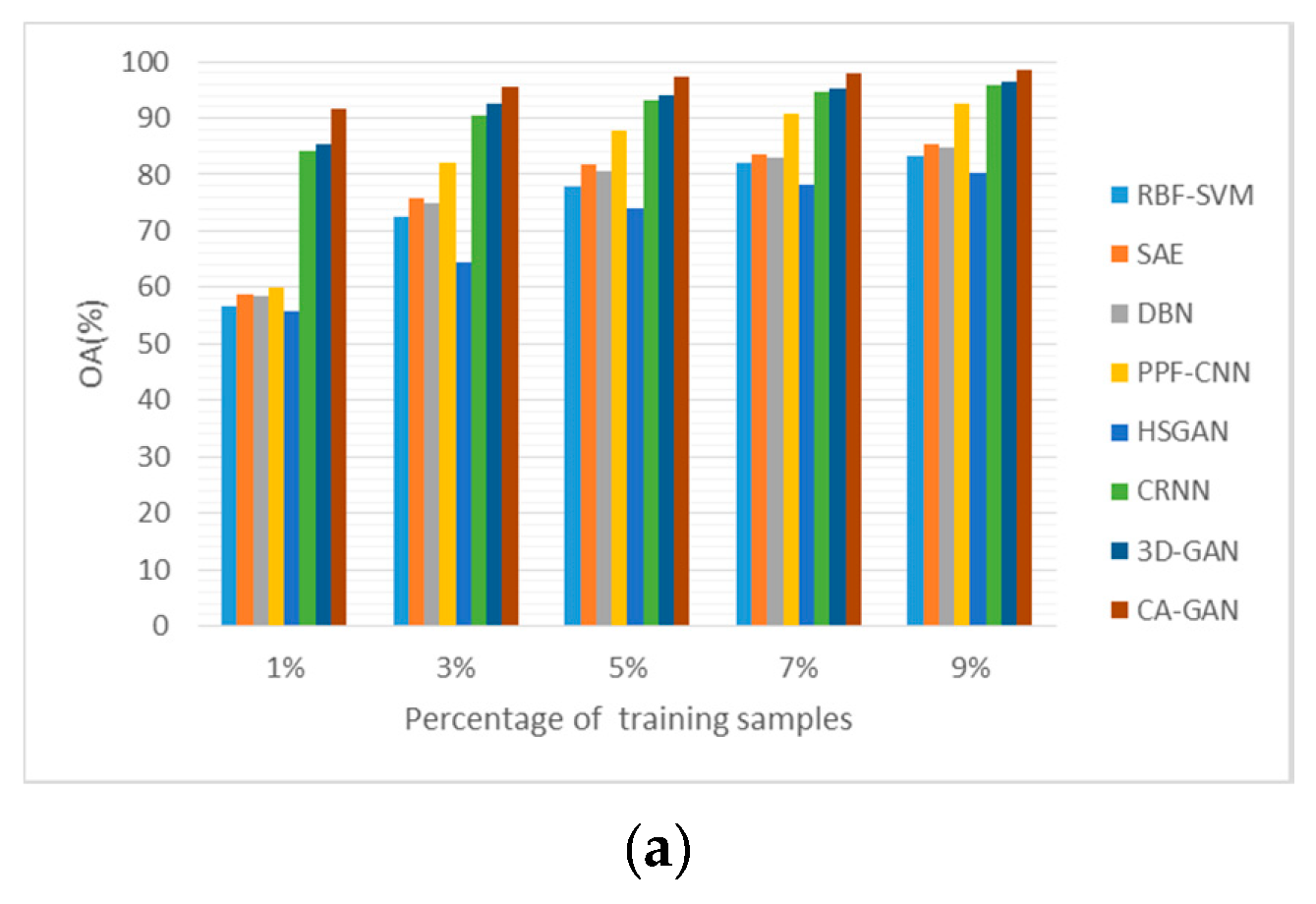
4.5. Sensitivity to the Proportion of Training Samples

To investigate the classification accuracies with different percentages of training samples, we change the percentage of training samples for each class from 1% to 9% at 2% intervals on the Indian Pines dataset. Similarly, the percentage of training samples for each class ranges from 1% to 5% at a 1% interval on the Pavia University and Washington datasets. Figure 10 shows the OAs of all the comparison algorithms with various percentages of training samples.

From Figure 10, the classification accuracy of the eight methods goes up quickly with the increase of the percentage of training samples. When the training samples are large enough, the classification accuracy of all the comparison methods changes slowly and tends to be stable. 3D-GAN and CA-GAN outperform RBF-SVM, SAE, DBN, CRNN, PPF-CNN, and HSGAN in three datasets with different percentages of training samples. Compared with PPF-CNN, HSGAN, and 3D-GAN, CA-GAN consistently provide excellent classification performance with different percentages. When the proportion of training samples is only 1%, CA-GAN increases by at least 6.1%, 5.6%, and 5.5% on three datasets, respectively. Thus, CA-GAN is suitable for the limited number of training samples.

4.6. Influence of Different Number of Principle Components in CA-GAN

To verify the effectiveness of the proposed method with different numbers of principal components, we change the number of principal components in PCA.

Table 12. The classification results of CA-GAN with different principal components of principal component analysis (PCA) on the Indian Pines dataset.

Dataset	CA-GAN Method	OA (%)	Training Time (s)
Indian Pines	PCA-20	97.4 ± 0.5	712.9 ± 3.1
	PCA-50	97.6 ± 0.3	1296.8 ± 59.8
	PCA-100	97.4 ± 0.3	2183.2 ± 101.7
	PCA-150	97.3 ± 0.2	3924.7 ± 241.5
	without PCA	97.1 ± 0.5	6396.8 ± 148.3

,

Table 13. The classification results of CA-GAN with different principal components of PCA on the Pavia University dataset.

Dataset	CA-GAN Method	OA (%)	Training Time (s)
Pavia University	PCA-20	99.2 ± 0.6	949.9 ± 80.2
	PCA-40	99.4 ± 0.4	1457.1 ± 83.4
	PCA-60	99.3 ± 0.4	2676.8 ± 129.8
	PCA-80	99.1 ± 0.3	4713.4 ± 185.3
	without PCA	99.0 ± 0.5	8034.8 ± 192.1

and

Table 14. The classification results of CA-GAN with different principal components of PCA on the Washington dataset.

Dataset	CA-GAN Method	OA (%)	Training Time (s)
Washington	PCA-20	99.5 ± 0.5	814.2 ± 7.2
	PCA-50	99.8 ± 0.2	1389.4 ± 36.8
	PCA-100	99.5 ± 0.3	2435.4 ± 74.1
	PCA-150	99.4 ± 0.2	4382.1 ± 183.5
	without PCA	99.2 ± 0.4	7274.1 ± 278.4

record the classification results and training time of the proposed method under various numbers of PCA components and the proposed method without PCA-based pre-processing.

As shown in Table 12, Table 13 and Table 14, the classification accuracy of CA-GAN on the three datasets increases firstly and then decreases with the increasing dimensionality of PCA. Compared with CA-GAN with PCA-20, CA-GAN with PCA-50 improves by 0.2%, 0.2%, and 0.3% on the three datasets, respectively. Although the classification accuracy is improved to some extent, more principal components lead to higher computational complexity and a longer training time. The training time of CA-GAN with PCA-50 is much longer than that of CA-GAN with PCA-20. When the principal components of PCA are further increased, the classification performance deteriorates slightly.

4.7. Effectiveness of Each Step in CA-GAN

Table 15. Effect of each step in CA-GAN on three datasets. CA-GAN-WC: CA-GAN without ConvLSTM, CA-GAN-WCA: CA-GAN without ConvLSTM and attention module, and CA-GAN-WCAC: CA-GAN without ConvLSTM, attention module and collaborative learning.

Dataset	Method	CA-GAN-WCAC	CA-GAN-WCA	CA-GAN-WC	CA-GAN
Indian Pines	OA (%)	94.0 ± 0.1	96.0 ± 0.3	97.0 ± 0.1	97.4 ± 0.5
	AA (%)	89.9 ± 1.6	94.2 ± 0.5	94.7 ± 0.8	95.2 ± 2.2
	Kappa (%)	92.3 ± 2.0	96.0 ± 0.1	96.6 ± 0.2	97.0 ± 0.6
Pavia University	OA (%)	96.0 ± 0.1	97.4 ± 0.5	98.7 ± 0.4	99.2 ± 0.6
	AA (%)	95.9 ± 0.2	97.1 ± 0.1	98.0 ± 0.3	98.6 ± 1.2
	Kappa (%)	96.0 ± 0.4	97.3 ± 1.0	98.5 ± 0.2	99.2 ± 0.7
Washington	OA (%)	96.3 ± 0.1	97.8 ± 0.3	99.1 ± 0.4	99.5 ± 0.5
	AA (%)	96.1 ± 0.2	97.5 ± 0.6	98.3 ± 0.1	98.9 ± 0.7
	Kappa (%)	96.3 ± 0.1	97.6 ± 0.1	98.8 ± 0.4	99.2 ± 0.4

records the results of verifying the validity of each step in the CA-GAN method. The comparison methods include CA-GAN without ConvLSTM (CA-GAN-WC), CA-GAN without ConvLSTM and attention module (CA-GAN-WCA), and CA-GAN without ConvLSTM, attention module and collaborative learning (CA-GAN-WCAC). As shown in Table 15, compared with CA-GAN-WCAC, CA-GAN-WCA increases by 2.0%, 1.4%, and 1.5% in the OA index on three datasets. It shows that collaborative learning can effectively improve the classification performance. Compared with CA-GAN-WCA, CA-GAN-WC improves by 1.0%, 1.3%, and 1.3% in the OA index on three datasets. It indicates adding the joint spatial–spectral hard attention module can facilitate the classification performance by improving the quality of generated samples. Compared with CA-GAN-WC, CA-GAN uses ConvLSTM to promote the classification performance by extracting joint spatial–spectral features of HSIs. Compared with CA-GAN-WC, CA-GAN-WCA, and CA-GAN-WCAC, CA-GAN shows the best classification results in the AA, OA, and Kappa on three datasets.

5. Conclusions

In this paper, a novel CA-GAN method has been designed to solve the small sample problem in HSI classification. In the generator, a joint spatial–spectral hard attention module is devised to discard misleading and confounding features of the generated samples and impel the distribution of generated samples to approximate the distribution of real HSIs. In the discriminator, a convolutional LSTM layer is merged in the discriminator to extract joint spatial–spectral information of HSIs. Additionally, a collaborative learning mechanism is designed to assist the sample generation in the generator by using the real sample information extracted by the discriminator. It enables the generator and discriminator to be optimized alternately not only through the competition but also in a collaborative manner. These designs enable CA-GAN to improve the classification performance of HSIs with limited training samples by using the high-quality generated samples. The experiment results invalidated that CA-GAN can obtain greater HSI classification results compared with other advanced methods. In the future, we will investigate how to determine the positions and numbers of various modules in CA-GAN more effectively and automatically. In addition, we will try other types of sampling strategies to reduce the overlap between the training and testing sets of HSIs.

References

1. Chang, C.I. Hyperspectral Data Exploitation: Theory and Applications; Wiley: Hoboken, NJ, USA, 2007; pp. 441–442. [Google Scholar]
2. Makki, I.; Younes, R.; Francis, C.; Bianchi, T.; Zucchetti, M. A survey of landmine detection using hyperspectral imaging. ISPRS J. Photogramm. Remote Sens. 2017, 124, 40–53. [Google Scholar] [CrossRef]
3. Gevaert, C.M.; Suomalainen, J.; Tang, J.; Kooistra, L. Generation of spectral-temporal response surfaces by combining multispectral satellite and hyperspectral UAV imagery for precision agriculture applications. IEEE J. Sel. Topics Appl. Earth Observ. Remote Sens. 2015, 8, 3140–3146. [Google Scholar] [CrossRef]
4. Brown, A.J.; Walter, M.R.; Cudahy, T.J. Hyperspectral imaging spectroscopy of a Mars analogue environment at the North Pole Dome, Pilbara Craton, Western Australia. Austral. J. Earth Sci. 2005, 52, 353–364. [Google Scholar] [CrossRef]
5. Kang, X.D.; Xiang, X.L.; Li, S.T.; Benediktsson, J.A. PCA-based edge-preserving features for hyperspectral image classification. IEEE Trans. Geosci. Remote Sens. 2017, 55, 7140–7151. [Google Scholar] [CrossRef]
6. Dong, Y.; Du, B.; Zhang, L.; Zhang, L. Dimensionality reduction and classification of hyperspectral images using ensemble discriminative local metric learning. IEEE Trans. Geosci. Remote Sens. 2017, 55, 2509–2524. [Google Scholar] [CrossRef]
7. Chen, P.; Jiao, L.; Liu, F.; Gou, S.; Zhao, J.; Zhao, Z. Dimensionality reduction of hyperspectral imagery using sparse graph learning. IEEE J. Sel. Topics Appl. Earth Observ. Remote Sens. 2017, 10, 1165–1181. [Google Scholar] [CrossRef]
8. Gu, Y.; Liu, T.; Jia, X.; Benediktsson, J.A.; Chanussot, J. Nonlinear multiple kernel learning with multiple-structure-element extended morphological profiles for hyperspectral image classification. IEEE Trans. Geosci. Remote Sens. 2016, 54, 3235–3247. [Google Scholar] [CrossRef]
9. Xue, Z.; Li, J.; Cheng, L.; Du, P. Spectral-spatial classification of hyperspectral data via morphological component analysis-based image separation. IEEE Trans. Geosci. Remote Sens. 2015, 53, 70–84. [Google Scholar]
10. Jia, S.; Zhang, X.; Li, Q. Spectral-Spatial Hyperspectral Image Classification Using Regularized Low-Rank Representation and Sparse Representation-Based Graph Cuts. IEEE J. Sel. Topics Appl. Earth Observ. Remote Sens. 2015, 8, 2473–2484. [Google Scholar] [CrossRef]
11. Fang, L.; Li, S.; Duan, W.; Ren, J.; Benediktsson, J.A. Classification of hyperspectral images by exploiting spectral-spatial information of superpixel via multiple kernels. IEEE Trans. Geosci. Remote Sens. 2015, 53, 6663–6674. [Google Scholar] [CrossRef] [Green Version]
12. Fang, L.; Li, S.; Kang, X.; Benediktsson, J.A. Spectral-spatial classification of hyperspectral images with a superpixel-based discriminative sparse model. IEEE Trans. Geosci. Remote Sens. 2015, 53, 4186–4201. [Google Scholar] [CrossRef]
13. Liu, J.; Wu, Z.; Wei, Z.; Xiao, L.; Sun, L. Spatial-spectral kernel sparse representation for hyperspectral image classification. IEEE J. Sel. Top. Appl. Earth Obs. Remote Sens. 2013, 6, 2462–2471. [Google Scholar] [CrossRef]
14. Chen, Y.; Nasrabadi, N.M.; Tran, T.D. Hyperspectral image classification using dictionary-based sparse representation. IEEE Trans. Geosci. Remote Sens. 2011, 49, 3973–3985. [Google Scholar] [CrossRef]
15. Delalieux, S.; Somers, B.; Haest, B.; Spanhove, T.; Borre, J.V.; Mücher, C.A. Heathland conservation status mapping through integration of hyperspectral mixture analysis and decision tree classifiers. Remote Sens. 2012, 126, 222–231. [Google Scholar] [CrossRef]
16. Melgani, F.; Bruzzone, L. Classification of hyperspectral remote sensing images with support vector machines. IEEE Trans. Geosci. Remote Sens. 2004, 42, 1778–1790. [Google Scholar] [CrossRef] [Green Version]
17. Gualtieriand, J.A.; Chettri, S. Support vector machines for classification of hyperspectral data. In Proceedings of the IEEE International Geoscience and Remote Sensing Symposium (IGARSS), Honolulu, HI, USA, 24–28 July 2000; pp. 813–815. [Google Scholar]
18. Zhong, S.; Chang, C.I.; Zhang, Y. Iterative Support Vector Machine for Hyperspectral Image Classification. In Proceedings of the 25th IEEE International Conference on Image Processing (ICIP), Athens, Greece, 7–10 October 2018; pp. 3309–3312. [Google Scholar]
19. Ham, J.; Chen, Y.; Crawford, M.M.; Ghosh, J. Investigation of the random forest framework for classification of hyperspectral data. IEEE Trans. Geosci. Remote Sens. 2005, 43, 492–501. [Google Scholar] [CrossRef] [Green Version]
20. Chen, Y.; Lin, Z.; Zhao, X.; Wang, G.; Gu, Y. Deep learning-based classification of hyperspectral data. IEEE J. Sel. Topics Appl. Earth Observ. Remote Sens. 2014, 7, 2094–2107. [Google Scholar] [CrossRef]
21. Jia, K.; Sun, L.; Gao, S.; Song, Z.; Shi, B.E. Laplacian auto-encoders: An explicit learning of nonlinear data manifold. Neurocomputing 2015, 160, 250–260. [Google Scholar] [CrossRef]
22. Zabalza, J.; Ren, J.; Zheng, J.; Zhao, H.; Qing, C.; Yang, Z.; Marshall, S. Novel segmented stacked autoencoder for effective dimensionality reduction and feature extraction in hyperspectral imaging. Neurocomputer 2016, 185, 1–10. [Google Scholar] [CrossRef] [Green Version]
23. Zhou, P.; Han, J.; Cheng, G.; Zhang, B. Learning compact and discriminative stacked autoencoder for hyperspectral image classification. IEEE Trans. Geosci. Remote Sens. 2019, 57, 4823–4833. [Google Scholar] [CrossRef]
24. Chen, Y.S.; Zhao, X.; Jia, X. Spectral-spatial classification of hyperspectral data based on deep belief network. IEEE J. Sel. Top. Appl. Earth Obs. Remote Sens. 2015, 8, 2381–2392. [Google Scholar] [CrossRef]
25. Zhong, P.; Gong, Z.; Li, S.; Schönlieb, C.B. Learning to diversify deep belief networks for hyperspectral image classification. IEEE Trans. Geosci. Remote Sens. 2017, 55, 3516–3530. [Google Scholar] [CrossRef]
26. Ghassemi, M.; Ghassemian, H.; Imani, M. Deep Belief Networks for Feature Fusion in Hyperspectral Image Classification. In Proceedings of the IEEE International Conference on Aerospace Electronics and Remote Sensing Technology (ICARES), Bali, Indonesia, 20–21 September 2018; pp. 1–6. [Google Scholar]
27. Mughees, A.; Tao, L. Multiple deep-belief-network-based spectral-spatial classification of hyperspectral images. Tsinghua Sci. Technol. 2018, 24, 183–194. [Google Scholar] [CrossRef]
28. Zhang, H.; Li, Y.; Zhang, Y.; Shen, Q. Spectral-spatial classification of hyperspectral imagery using a dual-channel convolutional neural network. Remote Sens. Lett. 2017, 8, 438–447. [Google Scholar] [CrossRef] [Green Version]
29. Chen, Y.S.; Jiang, H.L.; Li, C.Y. Deep feature extraction and classification of hyperspectral images based on convolutional neural networks. IEEE Trans. Geosci. Remote Sens. 2016, 54, 6232–6251. [Google Scholar] [CrossRef] [Green Version]
30. Wu, H.; Prasad, S. Convolutional recurrent neural networks for hyperspectral data classification. Remote Sens. 2017, 9, 298. [Google Scholar] [CrossRef] [Green Version]
31. Song, W.; Li, S.; Fang, L.; Lu, T. Hyperspectral image classification with deep feature fusion network. IEEE Trans. Geosci. Remote Sens. 2018, 56, 3173–3184. [Google Scholar] [CrossRef]
32. Lee, H.; Kwon, H. Going deeper with contextual CNN for hyperspectral image classification. IEEE Trans. Image Process. 2017, 26, 4843–4855. [Google Scholar] [CrossRef] [Green Version]
33. Zhong, Z.; Li, J.; Luo, Z.; Chapman, M. Spectral-spatial residual network for hyperspectral image classification: A 3-D deep learning framework. IEEE Trans. Geosci. Remote Sens. 2017, 56, 847–858. [Google Scholar] [CrossRef]
34. Li, W.; Wu, G.; Zhang, F.; Du, Q. Hyperspectral image classification using deep pixel-pair features. IEEE Trans. Geosci. Remote Sens. 2017, 55, 844–853. [Google Scholar] [CrossRef]
35. Goodfellow, I.; Pouget-Abadie, J.; Mirza, M.; Xu, B.; Warde-Farley, D.; Ozair, S.; Bengio, Y. Generative adversarial nets. In Proceedings of the Advances in Neural Information Processing Systems, Montreal, QC, Canada, 8–13 December 2014; pp. 2672–2680. [Google Scholar]
36. Reed, S.; Akata, Z.; Yan, X.; Logeswaran, L.; Schiele, B.; Lee, H. Generative adversarial text-to-image synthesis. In Proceedings of the International Conference on Machine Learning, New York, NY, USA, 19–24 June 2016. [Google Scholar]
37. Mathieu, M.; Couprie, C.; LeCun, Y. Deep multi-scale video prediction beyond mean square error. In Proceedings of the International Conference on Learning Representations, San Juan, Puerto Rico, 2–4 May 2016. [Google Scholar]
38. Isola, P.; Zhu, J.Y.; Zhou, T.; Efros, A.A. Image-to-image translation with conditional adversarial networks. In Proceedings of the IEEE Conference on Computer Vision and Pattern Recognition, Honolulu, HI, USA, 21–26 July 2017. [Google Scholar]
39. Che, T.; Li, Y.; Zhang, R.; Hjelm, R.D.; Li, W.; Song, Y.; Bengio, Y. Maximum-likelihood augmented discrete generative adversarial networks. arXiv 2017, arXiv:1702.07983. [Google Scholar]
40. Radford, A.; Metz, L.; Chintala, S. Unsupervised representation learning with deep convolutional generative adversarial networks. arXiv 2015, arXiv:1511.06434. [Google Scholar]
41. Arjovsky, M.; Chintala, S.; Bottou, L. Wasserstein generative adversarial networks. In Proceedings of the 34 th International Conference on Machine Learning (ICML), Sydney, Australia, 6–11 August 2017; pp. 214–223. [Google Scholar]
42. Gulrajani, I.; Ahmed, F.; Arjovsky, M.; Dumoulin, V.; Courville, A. Improved training of Wasserstein GANs. In Proceedings of the Advances in Neural Information Processing Systems. (NIPS), Long Beach, CA, USA, 4–9 December 2017; pp. 5769–5779. [Google Scholar]
43. Zhao, J.; Mathieu, M.; LeCun, Y. Energy-based generative adversarial network. In Proceedings of the International Conference on Learning Representations. (ICLR), Toulon, France, 24–26 April 2017; pp. 1–17. [Google Scholar]
44. Wang, D.; Vinson, R.; Holmes, M.; Seibel, G.; Bechar, A.; Nof, S.; Tao, Y. Early Tomato Spotted Wilt Virus Detection using Hyperspectral Imaging Technique and Outlier Removal Auxiliary Classifier Generative Adversarial Nets (OR-AC-GAN). In 2018 ASABE Annual International Meeting; American Society of Agricultural and Biological Engineers: St. Joseph, MI, USA, 2018; p. 1. [Google Scholar]
45. Ma, D.; Tang, P.; Zhao, L. SiftingGAN: Generating and sifting labeled samples to improve the remote sensing image scene classification baseline in vitro. IEEE Geosci. Remote Sens. Lett. 2019, 16, 1046–1050. [Google Scholar] [CrossRef] [Green Version]
46. Denton, E.; Chintala, S.; Szlam, A.; Fergus, R. Deep generative image models using a laplacian pyramid of adversarial networks. arXiv 2015, arXiv:1506.05751. [Google Scholar]
47. Radford, A.; Metz, L.; Chintala, S. Unsupervised representation learning with deep convolutional generative adversarial networks. In Proceedings of the International Conference on Learning Representations ICLR, Toulon, France, 20 January 2016; pp. 1–16. [Google Scholar]
48. Durugkar, I.; Gemp, I.; Mahadevan, S. Generative multi-adversarial networks. In Proceedings of the International Conference on Learning Representations. (ICLR), Toulon, France, 24–26 April 2017; pp. 1–14. [Google Scholar]
49. Neyshabur, B.; Bhojanapalli, S.; Chakrabarti, A. Stabilizing GAN Training With Multiple Random Projections. arXiv 2017, arXiv:1705.07831. [Google Scholar]
50. Salimans, T.; Goodfellow, I.; Zaremba, W.; Cheung, V.; Radford, A.; Chen, X. Improved techniques for training GANs. In Proceedings of the Advances in Neural Information Processing Systems, Barcelona, Spain, 5–10 December 2016; pp. 2234–2242. [Google Scholar]
51. Zhong, Z.; Li, J.; Clausi, D.A.; Wong, A. Generative adversarial networks and conditional random fields for hyperspectral image classification. IEEE Trans. Cybernetics 2019, 1–12. [Google Scholar] [CrossRef] [Green Version]
52. He, Z.; Liu, H.; Wang, Y.; Hu, J. Generative adversarial networks-based semi-supervised learning for hyperspectral image classification. Remote Sens. 2017, 9, 1042. [Google Scholar] [CrossRef] [Green Version]
53. Zhan, Y.; Hu, D.; Wang, Y.; Yu, X. Semisupervised hyperspectral image classification based on generative adversarial networks. IEEE Geosci. Remote Sens. Lett. 2018, 15, 212–216. [Google Scholar] [CrossRef]
54. Zhan, Y.; Wu, K.; Liu, W.; Qin, J.; Yang, Z.; Medjadba, Y.; Yu, X. Semi-supervised classification of hyperspectral data based on generative adversarial networks and neighborhood majority voting. In Proceedings of the IGARSS 2018-2018 IEEE International Geoscience and Remote Sensing Symposium, Valencia, Spain, 22–27 July 2018; pp. 5756–5759. [Google Scholar]
55. Zhan, Y.; Qin, J.; Huang, T.; Wu, K.; Hu, D.; Zhao, Z.; Wang, G. Hyperspectral Image Classification Based on Generative Adversarial Networks with Feature Fusing and Dynamic Neighborhood Voting Mechanism. In Proceedings of the IGARSS 2019-2019 IEEE International Geoscience and Remote Sensing Symposium, Yokohama, Japan, 28 July–2 August 2019; pp. 811–814. [Google Scholar]
56. Gao, H.; Yao, D.; Wang, M.; Li, C.; Liu, H.; Hua, Z.; Wang, J. A Hyperspectral Image Classification Method Based on Multi-Discriminator Generative Adversarial Networks. Sensors 2019, 19, 3269. [Google Scholar] [CrossRef] [Green Version]
57. Zhu, L.; Chen, Y.; Ghamisi, P.; Benediktsson, J.A. Generative adversarial networks for hyperspectral image classification. IEEE Trans. Geosci. Remote Sens. 2018, 56, 5046–5063. [Google Scholar] [CrossRef]
58. Feng, J.; Yu, H.; Wang, L.; Cao, X.; Zhang, X.; Jiao, L. Classification of Hyperspectral Images Based on Multiclass Spatial-Spectral Generative Adversarial Networks. IEEE Trans. Geosci. Remote Sens. 2019, 57, 5329–5343. [Google Scholar] [CrossRef]
59. Shi, X.; Chen, Z.; Wang, H.; Yeung, D.Y.; Wong, W.K.; Woo, W.C. Convolutional lstm network: A machine learning approach for precipitation nowcasting. In Proceedings of the Advances in Neural Information Processing Systems: Annual Conference on Neural Information Processing Systems (NIPS), Montreal, QC, Canada, 7–12 December 2015; pp. 802–810. [Google Scholar]
Figure 1. The original generative adversarial network (GAN) model.
Remotesensing 12 01149 g001
Figure 2. The framework of convolutional GAN based on collaborative learning and attention mechanism (CA-GAN).
Remotesensing 12 01149 g002
Figure 3. The joint spatial–spectral hard attention module.
Remotesensing 12 01149 g003
Figure 4. The discriminator in CA-GAN based on convolutional long short-term memory (Conv LSTM).
Remotesensing 12 01149 g004
Figure 5. False-color composite image. (a) Indian Pines, (b) Pavia University, and (c) Washington.
Remotesensing 12 01149 g005
Figure 6. Ground truth. (a) Indian Pines, (b) Pavia University, and (c) Washington.
Remotesensing 12 01149 g006
Figure 7. Classification visualization on the Indian Pines dataset obtained by (a) radial based function (RBF)-support vector machines (SVM); (b) stacked autoencoders (SAE); (c) deep belief networks (DBN); (d) pixel-pair features (PPF)-convolutional neural networks (CNN); (e) convolutional recurrent neural network (CRNN); (f) semi-supervised 1D-GAN algorithm (HSGAN); (g) 3D-GAN and (h) CA-GAN.
Remotesensing 12 01149 g007
Figure 8. Classification visualization on the Pavia University dataset obtained by (a) RBF-SVM, (b) SAE, (c) DBN, (d) PPF-CNN, (e) CRNN, (f) HSGAN, (g) 3D-GAN, and (h) CA-GAN.
Remotesensing 12 01149 g008
Figure 9. Classification visualization on the Washington obtained by (a) RBF-SVM; (b) SAE; (c) DBN; (d) PPF-CNN; (e) CRNN; (f) HSGAN; (g) 3D-GAN; and (h) CA-GAN.
Remotesensing 12 01149 g009
Figure 10. OA results of various methods with different percentages of training samples on the (a) Indian Pines Dataset, (b) Pavia University Dataset, and (c) Washington Dataset.
Remotesensing 12 01149 g010aRemotesensing 12 01149 g010b