Using Heterogeneous Satellites for Passive Detection of Moving Aerial Target

Abstract

Passive detection of a moving aerial target is critical for intelligent surveillance. Its implementation can use signals transmitted from satellites. Nowadays, various types of satellites co-exist which can be used for passive detection. As a result, a satellite signal receiver may receive signals from multiple heterogeneous satellites, causing difficult in echo signal detection. In this paper, a passive moving aerial target detection method leveraging signals from multiple heterogeneous satellites is proposed. In the proposed method, a plurality of direct wave signals is separated in a reference channel first. Then, an adaptive filter with normalized least-mean-square (NLMS) is adopted to suppress direct-path interference (DPI) and multi-path interference (MPI) in a surveillance channel. Next, the maximum values of the cross ambiguity function (CAF) and the fourth order cyclic cumulants cross ambiguity function (FOCCCAF) correspond into each separated direct wave signal and echo signal will be utilized as the detection statistic of each distributed sensor. Finally, final detection probabilities are calculated by decision fusion based on results from distributed sensors. To evaluate the performance of the proposed method, extensive simulation studies are conducted. The corresponding simulation results show that the proposed fusion detection method can significantly improve the reliability of moving aerial target detection using multiple heterogeneous satellites. Moveover, we also show that the proposed detection method is able to significantly improve the detection performance by using multiple collaborative heterogeneous satellites.

1. Introduction

Satellite communications have attracted tremendous attention in both industries and academia because of their significant advantages, such as all-weather operations, wide overage, strong viability, and high reliability [1,2]. To achieve globalization and performance enhancement, satellites have evolved from a single satellite model to a complicated system with multi-satellite concurrent compatibility. Accordingly, in addition to navigation in the traditional application of satellite systems, wireless communications and positioning can also be supported by current satellite systems. Recently, representative satellite systems, such as the global positioning system (GPS), the digital satellite broadcasting system (DVB-S) and the international maritime satellite (INMARSAT) have been widely used in military, industries, and human life [3].

Passive target detection using satellite illumination is an important application in satellite systems, which utilizes signals to detect moving targets through signal processing technologies [4,5]. Most existing works on passive target detection makes a strong assumption of a single satellite, in which only signals for a single satellite need to be processed [6,7,8,9,10]. However, in practice, a receiver in passive target detection is likely to receive illumination signals from different satellites. Thus, strong interference caused by undesired satellite illumination may greatly compromise the performance of traditional passive target detection methods designed for a single satellite illumination [9,11].

In order to adapt to the new multiple heterogeneous satellites environments, in this paper, we focus on developing the effective passive target detection method with multiple satellite illumination. Many technical challenges have to be addressed in this regard. For example, the first obstacle is interference suppression and expected signal purification. Specifically, a near-Earth orbit target may be simultaneously covered by multiple satellite beams and reference signals transmitted in a reference channel may be contaminated by unexpected signals, which makes the estimation of reference signals very difficult [12]. In addition, interference caused by other satellite signals may have negative impact on direct-path interference (DPI)/multi-path interference (MPI) suppression, resulting in poor subsequent echo detection performance in a surveillance channel [13]. Thus, multiple satellite signals received in the reference channel and the DPI/MPI in the surveillance channel should be purified and suppressed, respectively, for effective passive target detection.

Another challenge in passive target detection is that satellite signals received by a satellite signal receiver is generally weak. The huge propagation loss caused by the long-distance propagation from satellites to satellite signal receivers leads to a low received power [14,15]. Furthermore, satellite signals would be further weakened after being absorbed and reflected by a moving target, so-called target echo. Therefore, a long coherent accumulation time need to be taken to detect extremely weak satellite echo. To improve target detection probabilities, the viable option of developing a collaborative detection system using multiple heterogeneous satellite signals will be studied in this paper.

In our earlier work, a passive method leveraging signals from multiple homogeneous satellites was proposed for moving aerial target detection [16]. In this paper, a moving aerial target detection method utilizing multiple collaborative heterogeneous satellites is proposed. the main contributions of the paper are described as follows:

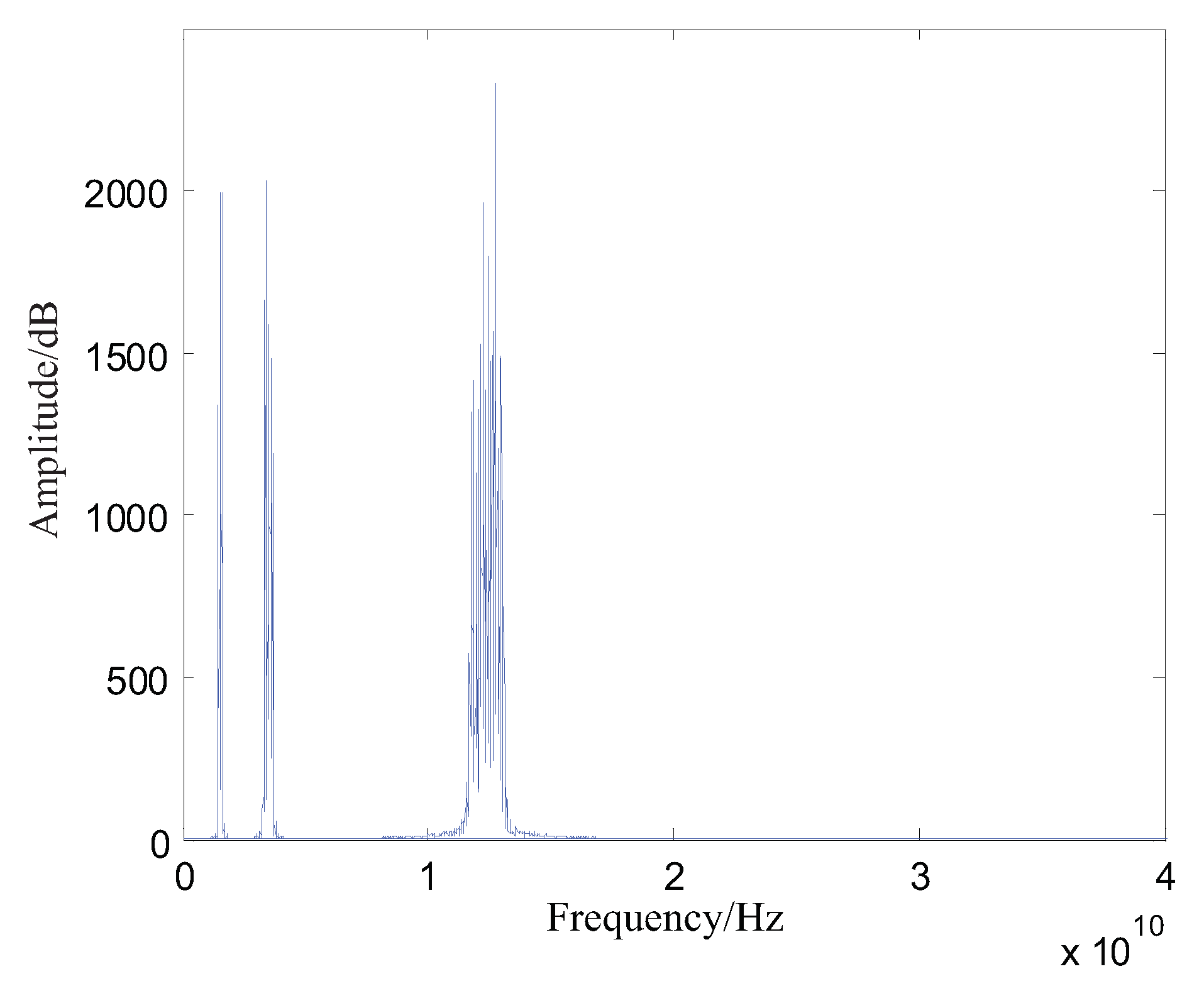
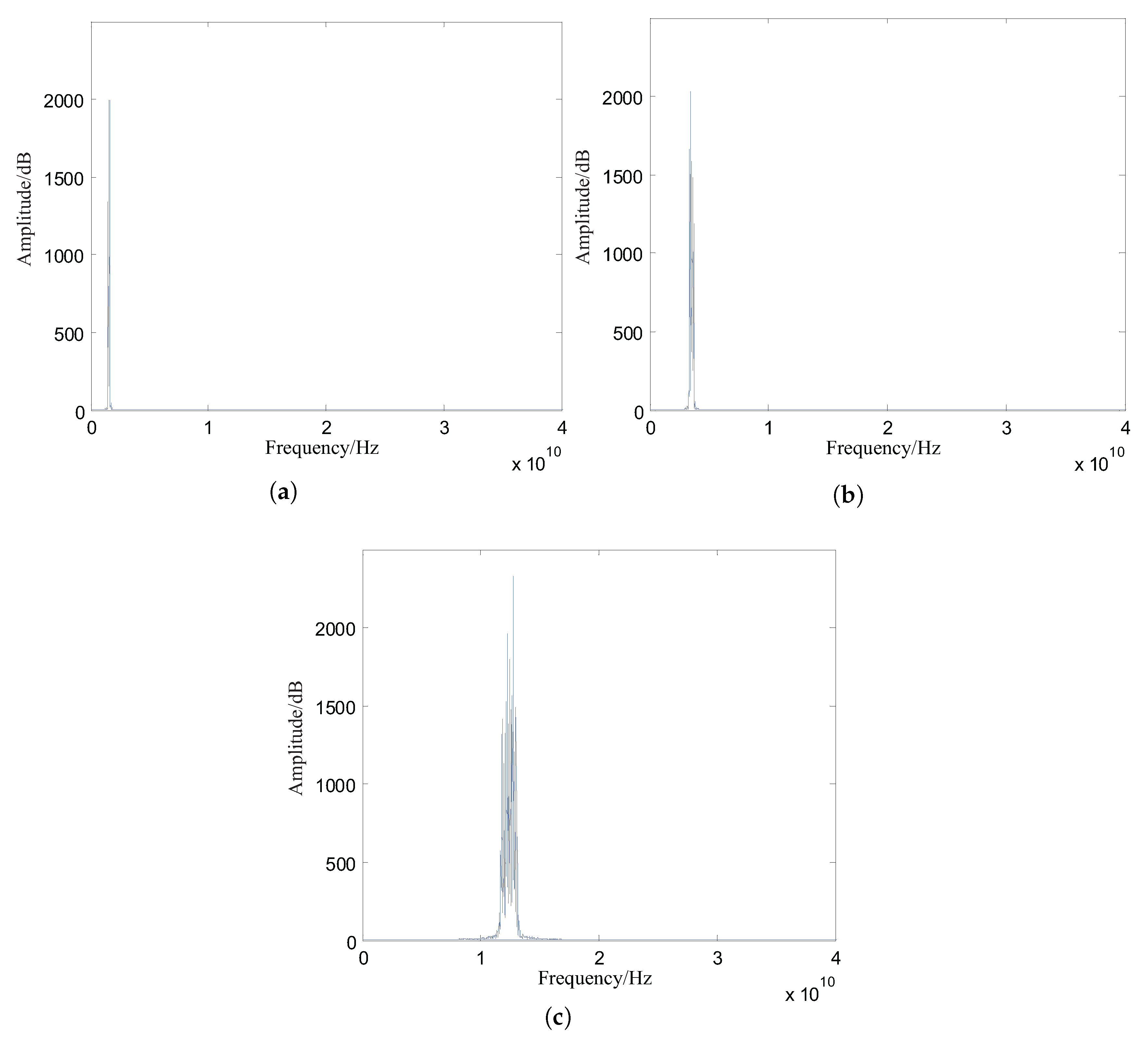
• For signal purification, parallel band-pass filters are employed to separate the direct wave signals in the reference channel. Moreover, an adaptive filter based on normalized least mean square (NLMS) is applied to suppress direct-path interference (DPI) and multi-path interference (MPI) in the surveillance channel.
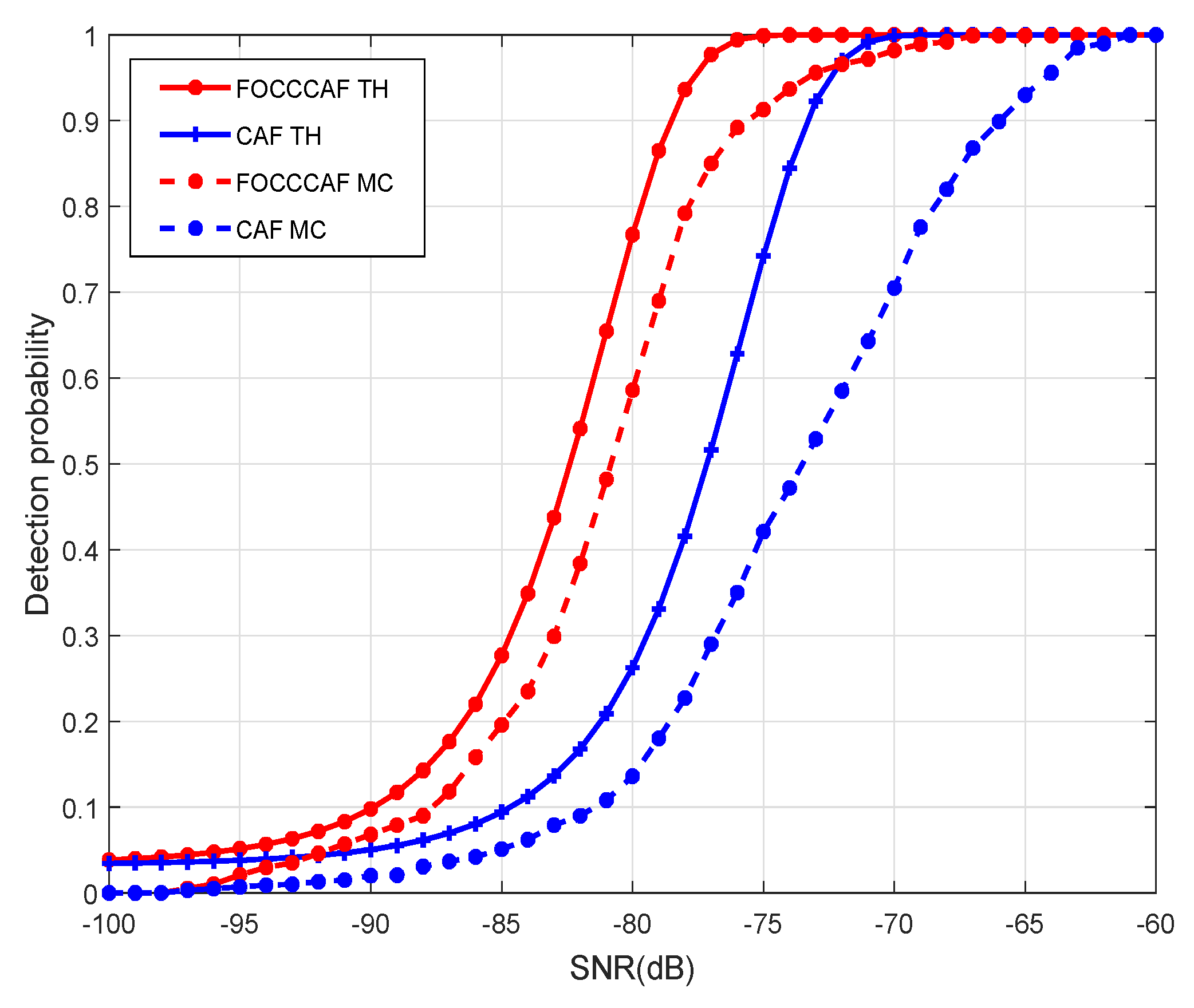
• The maximum value of the cross ambiguity function (CAF) and the fourth order cyclic cumulants cross ambiguity function (FOCCCAF) of each separated direct wave signal and the echo signal are used to improve the signal-to-noise ratio (SNR) of moving aerial target detection.
• Detection results are obtained by fusing the decisions of multiple sensors to enhance the reliability of moving aerial target detection.

The reminder of this paper is organized as follows. In Section 2, the system model used in this paper is presented. The separation of direct wave in the reference channel and suppression of DPI and MPI in the surveillance channel are described in Section 3. Detection statistics construction and the detector design are proposed in Section 4. In Section 5, the performance of the moving aerial target detection is analyzed. Section 6 shows the numerical results to verify the classification performance. Finally, Section 7 concludes the whole paper.

2. System Model

In this paper, a passive detection system, consisting of one moving aerial target, a satellite signal receiver, and multiple collaborative heterogeneous satellites is considered in the paper, as shown in Figure 1. The satellite signal receiver is comprised of a reference channel antenna and a surveillance channel antenna. The antenna dedicated to the reference channel receives direct wave signals from satellites, including GPS, DVB-S, and INMARSAT satellites. On the other hand, the antenna of the surveillance channel is used to receive target echo signals with the direct wave and multi-path interference.

In Figure 1, the signal $x\left(t\right)$ in the reference channel is given by [17]

$$x\left(t\right)={\displaystyle \sum _{i=1}^M}{r}_i{s}_i\left(t\right)+n\left(t\right),$$

(1)

where M denotes the number of different satellites, $n\left(t\right)$ is a statistically independent stationary Gaussian white noise with zero mean, $s_i\left(t\right)$ represents different direct wave signal from the i-th satellite, and $r_i$ stands for the amplitude of the different direct wave signal in the reference channel.

The signal $z\left(t\right)$ in the surveillance channel is expressed as

$$z\left(t\right)={\displaystyle \sum _{i=1}^M}{r^{\prime }}_i{s}_i(t-D_i)e^{-j2\pi f_{d_i}t}+{\displaystyle \sum _{i=1}^M}{\mathsf{\Omega }}_i{s}_i\left(t\right)+{\displaystyle \sum _{i=1}^M}{\displaystyle \sum _{j=1}^H}{\omega }_{ij}{s}_i(t-{\tau }_{ij})+n^{\prime }\left(t\right),$$

(2)

where ${r^{\prime }}_i$ is the amplitude of the i-th echo signal, $D_i$ represents the delay of the echo wave relative to the corresponding different direct wave, $f_{d_i}$ denotes the doppler shift of the echo of different direct wave signals, ${\mathsf{\Omega }}_i$ is the amplitude of the direct wave signal in the surveillance channel, ${\omega }_{ij}$ is the amplitude of the direct signal of the i-th satellite passing the j-th multipath channel. ${\tau }_{ij}$ stands for the direct signal of the i-th satellite after the j-th multipath channel. H represents the diameter of the multipath channel in the surveillance channel, $n^{\prime }\left(t\right)$ is a statistically independent stationary Gaussian white noise with zero mean.

3. Interference Suppression

3.1. Direct Wave Signal Separation in the Reference Channel

As the receiver in the reference channel receives multiple direct wave signals simultaneously, it is necessary to separate direct wave signals in the reference channel to facilitate suppression of DPI and MPI in the surveillance channel and subsequently process. Practically, GPS, DVB-S and INMARSAT satellites use different frequency bands to transmit signals. Therefore, different band-pass filters need to be used to separate various direct wave signals. The band-pass filter is determined by [18]    

$$H\left(e^{j\omega }\right)=\frac{{\displaystyle {\displaystyle \sum _{r=0}^Q}}{b}_r{\left(e^{j\omega }\right)}^{-r}}{1+{\displaystyle {\displaystyle \sum _{k=1}^S}}{a}_k{\left(e^{j\omega }\right)}^{-k}},$$

(3)

where $a_k$ and $b_r$ are the coefficient for the band-pass filter. ${\omega }_p$ denotes pass-band upper boundary frequency of the band-pass filter. ${\omega }_{pu}$ represents pass-band lower boundary frequency of the band-pass filter. ${\omega }_s$ stands for stop-band upper boundary frequency. ${\omega }_{su}$, ${\alpha }_p$, and ${\alpha }_s$ denote the stop-band lower boundary frequency, the pass-band maximum attenuation and the stop-band minimum attenuation, respectively. The parameters of different filters are set according to different spectral ranges, which determine the values of Q, S, $a_k$, $b_r$ of different band-pass filter system functions. Then, a plurality of band-pass filters are connected in parallel to separate direct wave signals at the same time to obtain different direct wave signals. After the separation of direct wave signals, the time-domain signals overlapped in the reference channel have become M independent direct wave signals, where the i-th direct wave signal $x_i\left(t\right)$ can be expressed as

$$x_i\left(t\right)=r_i{s}_i\left(t\right)+n\left(t\right).$$

(4)

The time-domain overlapped signals mixed with GPS, DVB-S and INMARSAT satellite signals in the reference channel are used for verification. The spectrogram of mixed direct wave signals is shown in Figure 2, while those of these three signals after separated by the band-pass filter are shown in Figure 3. From Figure 2 and Figure 3, it can be seen that after passing through the band-pass filter, the three satellite signals in time overlapped are effectively separated.

3.2. DPI and MPI Suppression Based on NLMS Adaptive Filter

The echo signals in the surveillance channel are extremely weak, while the power of DPI and MPI are much larger than that of echo signals. The gain obtained by increasing the coherent accumulation time can not satisfy the requirement of echo detection. Therefore, it is necessary to suppress the DPI and MPI in the surveillance channel.

The cascade suppression of DPI and MPI in the surveillance channel is achieved by using an adaptive filter [19,20,21]. The adaptive filter employs NLMS algorithm following [22]

$${\mathbf{e}}_{\mathbf{i}}\left(\mathbf{n}\right)={\mathbf{z}}_{\mathbf{i}}\left(\mathbf{n}\right)-{{\mathbf{x}}_{\mathbf{i}}}^{\mathbf{T}}\left(\mathbf{n}\right){\mathbf{w}}_{\mathbf{i}}\left(\mathbf{n}\right),$$

(5)

$${\mathbf{w}}_{\mathbf{i}}(\mathbf{n}+\mathbf{1})={\mathbf{w}}_{\mathbf{i}}\left(\mathbf{n}\right)+\frac{\mu }{\lambda +{∥{\mathbf{x}}_{\mathbf{i}}\left(\mathbf{n}\right)∥}^{\mathbf{2}}}{\mathbf{e}}_{\mathbf{i}}\left(\mathbf{n}\right){\mathbf{x}}_{\mathbf{i}}\left(\mathbf{n}\right),$$

(6)

where ${\mathbf{x}}_{\mathbf{i}}\left(\mathbf{n}\right)$ denotes the separation direct wave signal in the reference channel, ${\mathbf{z}}_{\mathbf{i}}\left(\mathbf{n}\right)$ represents the received signal of the surveillance channel, ${\mathbf{w}}_{\mathbf{i}}\left(\mathbf{n}\right)$ is the weight vector of the filter, and ${\mathbf{e}}_{\mathbf{i}}\left(\mathbf{n}\right)$ is the error signal. In order to avoid a very small ${∥{\mathbf{x}}_{\mathbf{i}}\left(\mathbf{n}\right)∥}^2$ that can cause divergence, $\lambda$ is set to a small positive constant and $\mu$ is the fixed normalized step factor with $0<\mu <2$.

The surveillance channel may contain a number of different direct wave signals and multi-path interference. Therefore, it is necessary to suppress the DPI and MPI one by one. The process of DPI and MPI suppression is as follows: the direct wave signal of each satellite is taken as an input signal ${\mathbf{x}}_{\mathbf{i}}\left(\mathbf{n}\right)$, firstly. Secondly, the output signal ${\mathbf{e}}_{\mathbf{i}}\left(\mathbf{n}\right)$ of the upper stage after the interference suppression by the adaptive filter is used as the training signal ${\mathbf{z}}_{\mathbf{i}}\left(\mathbf{n}\right)$ of the adaptive filter of the next stage. This process is repeated M times to complete cascade suppression of the DPI and MPI. Let $y\left(t\right)$ denote the signal in which the DPI and MPI are suppressed in the surveillance channel as

$$y\left(t\right)=z\left(t\right)-{\displaystyle \sum _{i=1}^M}{\displaystyle \sum _{j=0}^H}{w}_{ij}.x_i(t-j\mathsf{\Delta }),$$

(7)

where $w_{ij}$ represents the optimal weight of the j-th trajectory of the i-th satellite, and $j\mathsf{\Delta }$ stands for the delay of the j-th path. Thus, $y\left(t\right)$ contains only the echo signal of each satellite signal and Gaussian noise in the ideal case.

4. Detection Statistics Construction

4.1. Detection Statistic Construction Based on CAF

After the cascade NLMS adaptive filtering, there are only echo signals and Gaussian white noise in the surveillance channel. In order to detect the echo signals, the direct wave signal $x_i\left(t\right)$ after separation are correlated with the signal $y\left(t\right)$ of the surveillance channel after DPI and MPI suppression to obtain CAF, which is expressed as [23]

$${\chi }_i(\tau ,f_d)={\int }_0^{T_F}{x_i}^{\ast }(t-\tau )y\left(t\right)e^{j2\pi f_{d}t}dt,$$

(8)

where $\tau$ denotes time delay, $f_d$ is the Doppler shift, $T_F$ stands for coherent accumulation time. In this paper, several different doppler-time-delay spectra $\left|{\chi }_i(\tau ,f_d)\right|$ are obtained by Equation (8). Then we can construct the following detection statistic $\mathsf{\Lambda }$ as follows

$$\mathsf{\Lambda }=\left|{\chi }_i(\tau ,f_d)\right|.$$

(9)

4.2. Detection Statistic Construction Based on FOCCCAF

After the cascade NLMS adaptive filtering, the separated direct wave signal $x_i\left(t\right)$ and the signal $y\left(t\right)$ after the DPI and MPI suppression in the surveillance channel are processed based on FOCCCAF, which is expressed as

$${\chi }_{y,x_i}^{{\alpha }_i-f,{\alpha }_i}(u,f)={\int }_{-\infty }^{+\infty }{C}_{x_i{x}_i{x}_{i}y}^{{\alpha }_i-f}\left(\tau \right)C_{4x_i}^{{\alpha }_i}{(\tau -u)}^{\ast }{e}^{j\pi f\tau }d\tau ,$$

(10)

where $C_{4x_i}^{{\alpha }_i}\left(\tau \right)$ represents the fourth-order self-circulating cumulant of the direct wave $x_i\left(t\right)$, and the cyclic frequency is ${\alpha }_i$. $C_{x_i{x}_i{x}_{i}y}^{{\alpha }_{i-f}}\left(\tau \right)$ denotes the fourth-order mutual-circulating cumulant of $x_i\left(t\right)$ and $y\left(t\right)$, the cyclic frequency is ${\alpha }_i-f$. $C_{4x_i}^{{\alpha }_i}\left(\tau \right)$ is expressed as

$$C_{4x_i}^{{\alpha }_i}\left(\tau \right)=r_i^4{M}_{4s_i}^{{\alpha }_i}\left(\tau \right)-3A{r}_i^2{M}_{2s_i}^{{\alpha }_i}\left(\tau \right),$$

(11)

where A is the mean squared value of $s_i\left(t\right)$. $M_{4s_i}^{{\alpha }_i}\left(\tau \right)$ and $M_{2s_i}^{{\alpha }_i}\left(\tau \right)$ are the fourth-order cyclic moment and the second-order cyclic moment of $s_i\left(t\right)$ at ${\alpha }_i$, which can be expressed as

$$M_{4s_i}^{{\alpha }_i}\left(\tau \right)={\displaystyle \underset{T\to \infty }{lim}}\frac{1}{T}{\displaystyle \sum _{t=0}^{T-1}}\left(s_i\left(t\right)s_i\left(t\right)s_i\left(t\right)s_i(t+\tau )\right)e^{-j8\pi {\alpha }_{i}t},$$

(12)

$$M_{2s_i}^{{\alpha }_i}\left(\tau \right)={\displaystyle \underset{T\to \infty }{lim}}\frac{1}{T}{\displaystyle \sum _{t=0}^{T-1}}\left(s_i\left(t\right)s_i(t+\tau )\right)e^{-j4\pi {\alpha }_{i}t},$$

(13)

where T is the length of time. $C_{x_i{x}_i{x}_{i}y}^{{\alpha }_i-f}\left(\tau \right)$ is the fourth-order mutual-circulating cumulant of $x_i\left(t\right)$ and $y\left(t\right)$, which can be expressed as [24,25]

$$\begin{array}{c}{C}_{x_i{x}_i{x}_{i}y}^{{\alpha }_i-f}\left(\tau \right)=r_i^3{r}_i^{{}^{\prime }}{e}^{-j\pi ({\alpha }_i-f+f_{d_i})D_i}{M}_{4s_i}^{{\alpha }_i-f+f_{d_i}}(\tau -D_i)\hfill \\ +3r_i^2{r}_i^{{}^{\prime }}{e}^{-j\pi f_{d_i}\tau }{e}^{-j\pi ({\alpha }_i-f+f_{d_i})D_i}{M}_{s_i{s}_{i}n{s}_i}^{{\alpha }_i-f+f_{d_i}}(\tau -D_i)\hfill \\ -3B{r}_i^{}{r}_i^{{}^{\prime }}{e}^{-j\pi f_{d_i}\tau }{e}^{-j\pi ({\alpha }_i-f+f_{d_i})D_i}{R}_{s_i}^{{\alpha }_i-f+f_{d_i}}(\tau -D_i)\hfill \\ +r_i^3{M}_{s_i{s}_{i}n{s}_i}^{{\alpha }_i-f}\left(\tau \right),\hfill \end{array}$$

(14)

where $B=E\left[x_i\left(t\right)y\left(t\right)\right]$, ${\alpha }_i-f$ denotes the fourth-order mutual-cyclic frequency of $x_i\left(t\right)$ and $y\left(t\right)$. $R_{s_i}^{{\alpha }_i-f+f_{d_i}}(\tau -D_i)$ is the cyclic autocorrelation of the $i_{th}$ signal $s_i\left(t\right)$, which is given by

$$R_{s_i}^{{\alpha }_i-f+f_{d_i}}(\tau -D_i)={\displaystyle \underset{T\to \infty }{lim}}\frac{1}{T}{\displaystyle \sum _{t=0}^{T-1}}\left(s_i\left(t\right)s_i(t+\tau )\right)e^{-j2\pi {\alpha }_{i}t}.$$

(15)

$M_{4s_i}^{{\alpha }_i-f+f_{d_i}}(\tau -D_i)$ is the fourth-order mutual-circulating moment of $s_i\left(t\right)$ and $n\left(t\right)$ in the reference channel, which can be expressed as

$$M_{s_i{s}_{i}n{s}_i}^{{\alpha }_i-f+f_{d_i}}(\tau -D_i)={\displaystyle \underset{T\to \infty }{lim}}\frac{1}{T}{\displaystyle \sum _{t=0}^{T-1}}\left(s_i\left(t\right)s_i\left(t\right)n\left(t\right)s_i(t+\tau -D_i)\right)e^{-j2\pi ({\alpha }_i-f+f_{d_i})t}.$$

(16)

$M_{s_i{s}_{i}n{s}_i}^{{\alpha }_i-f}\left(\tau \right)$ is the fourth-order mutual-circulating moment of $s_i\left(t\right)$ and $n^{{}^{\prime }}\left(t\right)$, which can be expressed as

$$M_{s_i{s}_i{n}^{{}^{\prime }}{s}_i}^{{\alpha }_i-f+f_{d_i}}(\tau -D_i)={\displaystyle \underset{T\to \infty }{lim}}\frac{1}{T}{\displaystyle \sum _{t=0}^{T-1}}\left(s_i\left(t\right)s_i\left(t\right)n^{{}^{\prime }}\left(t\right)s_i(t+\tau -D_i)\right)e^{-j2\pi ({\alpha }_i-f+f_{d_i})t}.$$

(17)

Substituting Equation (11) and Equation (14) into Equation (10), we can obtain

$$\begin{array}{c}{\chi }_{y,x_i}^{{\alpha }_i-f,{\alpha }_i}(u,f)={\int }_{-\infty }^{+\infty }{C_{x_i{x}_i{x}_{i}y}^{{\alpha }_i-f}\left(C_{4x_i}^{{\alpha }_i}(\tau -u)\right)}^{\ast }{e}^{j\pi f\tau }d\tau \hfill \\ =r_i^7{r}_i^{{}^{\prime }}{e}^{-j\pi ({\alpha }_i-f+f_{d_i})D}{\int }_{-\infty }^{+\infty }{M}_{4s_i}^{{\alpha }_i-f+f_{d_i}}(\tau -D_i){\left(M_{4s_i}^{{\alpha }_i}(\tau -u)\right)}^{\ast }{e}^{j\pi (f-f_{d_i})\tau }d\tau \hfill \\ +9AB{r}_i^3{r}_i^{{}^{\prime }}{e}^{-j\pi ({\alpha }_i-f+f_{d_i})D}{\int }_{-\infty }^{+\infty }{R}_{s_i}^{{\alpha }_i-f+f_{d_i}}(\tau -D_i){\left(R_{s_i}^{{\alpha }_i}(\tau -u)\right)}^{\ast }{e}^{j\pi (f-f_{d_i})\tau }d\tau \hfill \\ -3B{r}_i^5{r}_i^{{}^{\prime }}{e}^{-j\pi ({\alpha }_i-f+f_{d_i})D}{\int }_{-\infty }^{+\infty }{\left(M_{4s_i}^{{\alpha }_i}(\tau -u)\right)}^{\ast }{R}_{s_i}^{{\alpha }_i-f+f_{d_i}}(\tau -D_i)e^{j\pi (f-f_{d_i})\tau }d\tau \hfill \\ -3A{r}_i^5{r}_i^{{}^{\prime }}{e}^{-j\pi ({\alpha }_i-f+f_{d_i})D}{\int }_{-\infty }^{+\infty }{M}_{4s_i}^{{\alpha }_i-f+f_{d_i}}(\tau -D_i){\left(R_{s_i}^{{\alpha }_i}(\tau -u)e^{j\pi (f-f_{d_i})\tau }\right)}^{\ast }d\tau \hfill \\ -9A{r}_i^4{r}_i^{{}^{\prime }}{e}^{-j\pi ({\alpha }_i-f+f_{d_i})D}{\int }_{-\infty }^{+\infty }{M}_{s_i{s}_{i}n{s}_i}^{{\alpha }_i-f+f_{d_i}}(\tau -D_i){\left(R_{s_i}^{{\alpha }_i}(\tau -u)e^{j\pi (f-f_{d_i})\tau }\right)}^{\ast }d\tau \hfill \\ +3r_i^6{r}_i^{{}^{\prime }}{e}^{-j\pi ({\alpha }_i-f+f_{d_i})D}{\int }_{-\infty }^{+\infty }{M}_{s_i{s}_{i}n{s}_i}^{{\alpha }_i-f+f_{d_i}}(\tau -D_i){\left(M_{4s_i}^{{\alpha }_i}(\tau -u)\right)}^{\ast }{e}^{j\pi (f-f_{d_i})\tau }d\tau \hfill \\ -3A{r}_i^5{\int }_{-\infty }^{+\infty }{M}_{s_i{s}_i{s}_i{n}^{{}^{\prime }}}^{{\alpha }_i-f}\left(\tau \right){\left(R_{s_i}^{{\alpha }_i}(\tau -u)e^{j\pi (f-f_{d_i})\tau }\right)}^{\ast }{e}^{j\pi f\tau }d\tau \hfill \\ +r_i^7{\int }_{-\infty }^{+\infty }{M}_{s_i{s}_i{s}_i{n}^{{}^{\prime }}}^{{\alpha }_i-f}\left(\tau \right){\left(M_{4s_i}^{{\alpha }_i}(\tau -u)\right)}^{\ast }{e}^{j\pi f\tau }d\tau .\hfill \end{array}$$

(18)

In Equation (18), the first four items do not contain any noise, which is used to detect the echo signal, and constructs the following detection statistic $\mathsf{\Lambda }$ as

$$\begin{array}{c}\mathsf{\Lambda }=r_i^7{r}_i^{{}^{\prime }}{e}^{-j\pi ({\alpha }_i-f+f_{d_i})D}{\int }_{-\infty }^{+\infty }{M}_{4s_i}^{{\alpha }_i-f+f_{d_i}}(\tau -D_i){\left(M_{4s_i}^{{\alpha }_i}(\tau -u)\right)}^{\ast }{e}^{j\pi (f-f_{d_i})\tau }d\tau \hfill \\ +9AB{r}_i^3{r}_i^{{}^{\prime }}{e}^{-j\pi ({\alpha }_i-f+f_{d_i})D}{\int }_{-\infty }^{+\infty }{R}_{s_i}^{{\alpha }_i-f+f_{d_i}}(\tau -D_i){\left(R_{s_i}^{{\alpha }_i}(\tau -u)\right)}^{\ast }{e}^{j\pi (f-f_{d_i})\tau }d\tau \hfill \\ -3B{r}_i^5{r}_i^{{}^{\prime }}{e}^{-j\pi ({\alpha }_i-f+f_{d_i})D}{\int }_{-\infty }^{+\infty }{\left(M_{4s_i}^{{\alpha }_i}(\tau -u)\right)}^{\ast }{R}_{s_i}^{{\alpha }_i-f+f_{d_i}}(\tau -D_i)e^{j\pi (f-f_{d_i})\tau }d\tau \hfill \\ -3A{r}_i^5{r}_i^{{}^{\prime }}{e}^{-j\pi ({\alpha }_i-f+f_{d_i})D}{\int }_{-\infty }^{+\infty }{M}_{4s_i}^{{\alpha }_i-f+f_{d_i}}(\tau -D_i){\left(R_{s_i}^{{\alpha }_i}(\tau -u)e^{j\pi (f-f_{d_i})\tau }\right)}^{\ast }d\tau .\hfill \end{array}$$

(19)

In Equation (19), let ${\rho }_{MR}$ denote the correlation coefficient of the fourth-order self-circulating moment $M_{4s_i}^{{\alpha }_i}\left(\tau \right)$ of the signal $s_i\left(t\right)$ and the cyclic autocorrelation function $R_{s_i}^{{\alpha }_i}\left(\tau \right)$ of $s_i\left(t\right)$ as

$${\rho }_{MR}=\frac{\mathrm{cov}(M_{4s_i}^{{\alpha }_i}\left(\tau \right),R_{s_i}^{{\alpha }_i}\left(\tau \right))}{\sqrt{\mathrm{var}\left(M_{4s_i}^{{\alpha }_i}\left(\tau \right)\right)}\sqrt{\mathrm{var}\left(R_{s_i}^{{\alpha }_i}\left(\tau \right)\right)}},$$

(20)

where $\mathrm{var}\left(M_{4s_i}^{{\alpha }_i}\left(\tau \right)\right)$ represents the variance of $M_{4s_i}^{{\alpha }_i}\left(\tau \right)$, $\mathrm{var}\left(R_{s_i}^{{\alpha }_i}\left(\tau \right)\right)$ denotes the variance of $R_{s_i}^{{\alpha }_i}\left(\tau \right)$, and $\mathrm{cov}(M_{4s_i}^{{\alpha }_i}\left(\tau \right),R_{s_i}^{{\alpha }_i}\left(\tau \right))$ is the covariance of $M_{4s_i}^{{\alpha }_i}\left(\tau \right)$ and $R_{s_i}^{{\alpha }_i}\left(\tau \right)$, which can be expressed as

$$\mathrm{cov}(M_{4s_i}^{{\alpha }_i}\left(\tau \right),R_{s_i}^{{\alpha }_i}\left(\tau \right))=E\left[M_{4s_i}^{{\alpha }_i}\left(\tau \right)R_{s_i}^{{\alpha }_i}\left(\tau \right)\right]-E\left[M_{4s_i}^{{\alpha }_i}\left(\tau \right)\right]E\left[R_{s_i}^{{\alpha }_i}\left(\tau \right)\right].$$

(21)

From Equation (12) and Equation (15), we can obtain

$$\begin{array}{c}E\left[M_{4s_i}^{{\alpha }_i}\left(\tau \right)R_{s_i}^{{\alpha }_i}\left(\tau \right)\right]\hfill \\ =E\left[{\displaystyle \underset{T\to \infty }{lim}}\left(\frac{1}{T}{\displaystyle \sum _{t=0}^{T-1}}\left(s_i\left(t\right)s_i\left(t\right)s_i\left(t\right)s_i(t+\tau )\right)e^{-j8\pi {\alpha }_{i}t}\frac{1}{T}{\displaystyle \sum _{t=0}^{T-1}}\left(s_i\left(t\right)s_i(t+\tau )\right)e^{-j2\pi {\alpha }_{i}t}\right)\right]\hfill \\ =E\left[{\displaystyle \underset{T\to \infty }{lim}}\left(\frac{1}{T}{\displaystyle \sum _{t=0}^{T-1}}\left(s_i\left(t\right)s_i\left(t\right)s_i\left(t\right)s_i\left(t\right)\right)e^{-j8\pi {\alpha }_{i}t}\right){\displaystyle \underset{T\to \infty }{lim}}\left(\frac{1}{T}{\displaystyle \sum _{t=0}^{T-1}}\left(s_i(t+\tau )s_i(t+\tau )\right)e^{-j2\pi {\alpha }_{i}t}\right)\right]\hfill \\ =E\left[M_{4s_i}^{{\alpha }_i}\left(\tau \right)\right]E\left[R_{s_i}^{{\alpha }_i}\left(\tau \right)\right].\hfill \end{array}$$

(22)

From the above analysis, we can obtain

$$\mathrm{cov}(M_{4s_i}^{{\alpha }_i}\left(\tau \right),R_{s_i}^{{\alpha }_i}\left(\tau \right))=E\left[M_{4s_i}^{{\alpha }_i}\left(\tau \right)R_{s_i}^{{\alpha }_i}\left(\tau \right)\right]-E\left[M_{4s_i}^{{\alpha }_i}\left(\tau \right)\right]E\left[R_{s_i}^{{\alpha }_i}\left(\tau \right)\right]=0.$$

(23)

Using Equation (23) in Equation (20), we can also obtain

$${\rho }_{MR}=0,$$

(24)

and Equation (19) can be simplified as

$$\begin{array}{c}\mathsf{\Lambda }=r_i^7{r}_i^{{}^{\prime }}{e}^{-j\pi ({\alpha }_i-f+f_{d_i})D}{\int }_{-\infty }^{+\infty }{M}_{4s_i}^{{\alpha }_i-f+f_{d_i}}(\tau -D_i){\left(M_{4s_i}^{{\alpha }_i}(\tau -u)\right)}^{\ast }{e}^{j\pi (f-f_{d_i})\tau }d\tau \hfill \\ +9AB{r}_i^3{r}_i^{{}^{\prime }}{e}^{-j\pi ({\alpha }_i-f+f_{d_i})D}{\int }_{-\infty }^{+\infty }{R}_{s_i}^{{\alpha }_i-f+f_{d_i}}(\tau -D_i){\left(R_{s_i}^{{\alpha }_i}(\tau -u)\right)}^{\ast }{e}^{j\pi (f-f_{d_i})\tau }d\tau .\hfill \end{array}$$

(25)

4.3. Detector Design

In order to improve the reliability of the final detection results, distributed sensors are used for collaborative detection. Each sensor is designed as a binary detector, whose binary hypothesis can be described as: assumption $H_1$ shows that the surveillance channel signal $y\left(t\right)$ contains the echo signal $r_i^{\prime }{s}_i(t-D_i)e^{-j2\pi f_{d_i}t}$ corresponding to the i-th direct wave signal $r_i{s}_i\left(t\right)$; assumption $H_0$ shows that the surveillance channel $y\left(t\right)$ does not contain the echo signal $r_i^{\prime }{s}_i(t-D_i)e^{-j2\pi f_{d_i}t}$ corresponding to the i-th direct wave $r_i{s}_i\left(t\right)$), which can be expressed as

$$\left\{\begin{array}{c}{H}_1:y\left(t\right)={\displaystyle \sum _{\genfrac{}{}{0pt}{}{\eta =1\hfill }{\exists \eta =i\hfill }}^M}{r}_{\eta }^{{}^{\prime }}{s}_{\eta }(t-D_{\eta })e^{-j2\pi f_{d_{\eta }}t}+n^{\prime }\left(t\right),\hfill \\ H_0:y\left(t\right)={\displaystyle \sum _{\genfrac{}{}{0pt}{}{\eta =1\hfill }{\forall \eta \ne i\hfill }}^M}{r}_{\eta }^{{}^{\prime }}{s}_{\eta }(t-D_{\eta })e^{-j2\pi f_{d_{\eta }}t}+n^{\prime }\left(t\right).\hfill \end{array}\right.$$

(26)

Based on the binary hypothesis in Equation (26), the binary detector is

$$\left|\mathsf{\Lambda }\right|\begin{array}{c}\stackrel{H_1}{>}\\ {\displaystyle \underset{H_0}{<}}\end{array}{T}_{d_i},$$

(27)

where $T_{d_i}$ is the detection threshold. Each sensor uses detector in Equation (27) to make the decision. Each sensor decision $u_i$ is

$$u_i=\left\{\begin{array}{cc}0\hfill & else,\\ 1\hfill & \mathsf{\Lambda }\ge T_{d_i}.\end{array}\right.$$

(28)

When output $u_i$ of the sensor is one, target is detected, and $H_1$ is true. When output $u_i$ of the sensor is zero, no target is detected, and $H_0$ is true. The performance of the $ith$ sensor can be denoted as $P(u_i/H_{j^{\prime }}),j^{\prime }=0,1$. The false alarm probability of the $ith$ sensor can be denoted as $P_i(1/H_0)=P_{f_i}$, the detection probability of the sensor can be denoted as $P_i(1/H_1)=P_{d_i}$. According to Equation (28), the fusion center of the distributed sensor fuses the decision result of each sensor according to the criterion of "h in k". It means that if there are more than or equal k sensors that detect the target in h sensors, the overall decision is $H_1$. The decision of each sensor is independent of each other, the fusion center gives the decision output u as

$$u=\left\{\begin{array}{cc}1\hfill & {\displaystyle \sum _{i=1}^h}{u}_i\ge k,\\ 0\hfill & else.\end{array}\right.$$

(29)

After the fusion decision of the fusion center, the final detection probability $P_d$ is expressed as

$$\begin{array}{c}{P}_d=P(u=1/H_1)\hfill \\ =P(u=1/u_{1,}{u}_{2,}\dots u_h,H_1)P(u_{1,}{u}_{2,}\dots u_h/H_1)\hfill \\ =P(u=1/u_{1,}{u}_{2,}\dots u_h,H_1){\displaystyle \prod _{i=1}^h}P(u_i/H_1)\hfill \\ =P(u=1/u_{1,}{u}_{2,}\dots u_h,H_1){\displaystyle \prod _{i\in S_1}}P(u_i=1/H_1){\displaystyle \prod _{i\in S_0}}P(u_i=0/H_1)\hfill \\ =P(u=1/u_{1,}{u}_{2,}\dots u_h,H_1){\displaystyle \prod _{i\in S_1}}{P}_{d_i}{\displaystyle \prod _{i\in S_0}}(1-P_{d_i})\hfill \\ ={\displaystyle \sum _{i^{\prime }=k}^h}{\displaystyle \sum _{C_{i^{\prime }/h}}}\{P_{d_1},P_{d_2},\cdots P_{d_h}\}\hfill \\ ={\displaystyle \sum _{i^{\prime }=k}^h}{\displaystyle \sum _{\sum u_i=i^{\prime }}}{\displaystyle \prod _i}{P_{d_i}}^{u_i}{(1-P_{d_i})}^{1-u_i},\hfill \end{array}$$

(30)

where $S_1=\left\{i\left|u_i=1,{\forall }_i=1,\cdots ,h\right.\right\}$, $S_0=\left\{i\left|u_i=0,{\forall }_i=1,\cdots ,h\right.\right\}$. The final false alarm probability $P_f$ is expressed as

$$\begin{array}{c}{P}_f=P(u=1/H_0)\hfill \\ =P(u=1/u_1,u_2,\dots u_h,H_0){\displaystyle \prod _{i\in S_1}}{P}_{f_i}{\displaystyle \prod _{i\in S_0}}(1-P_{f_i})\hfill \\ ={\displaystyle \sum _{i^{\prime }=k}^h}{\displaystyle \sum _{C_{i^{\prime }/h}}}\left\{P_{f_1},P_{f_2},\cdots ,P_{f_h}\right\}\hfill \\ ={\displaystyle \sum _{i^{\prime }=k}^h}{\displaystyle \sum _{\sum u_i=i^{\prime }}}{\displaystyle \prod _i}{P_{f_i}}^{u_i}{(1-P_{f_i})}^{1-u_i}.\hfill \end{array}$$

(31)

From the above, the procedure of the moving aerial target detection method based on multiple collaborative heterogeneous satellites is summarized in Algorithm 1.

Algorithm 1 The procedure of the proposed passive detection method.

1: Different direct wave signals in the reference channel are parallelly separated by Equation (3);   2: DPI and MPI are in the surveillance channel cascadely suppressed by Equation (5) and Equation (6);   3: FOCCCAF and CAF are introduced by Equation (10) and Equation (8) to construct the detection statistic $\mathsf{\Lambda }$;   4: Fuse the binary decision results of each sensor among the distributed sensors to get the final target detection results by Equation (29).

5. Moving Aerial Target Detection Performance Analysis

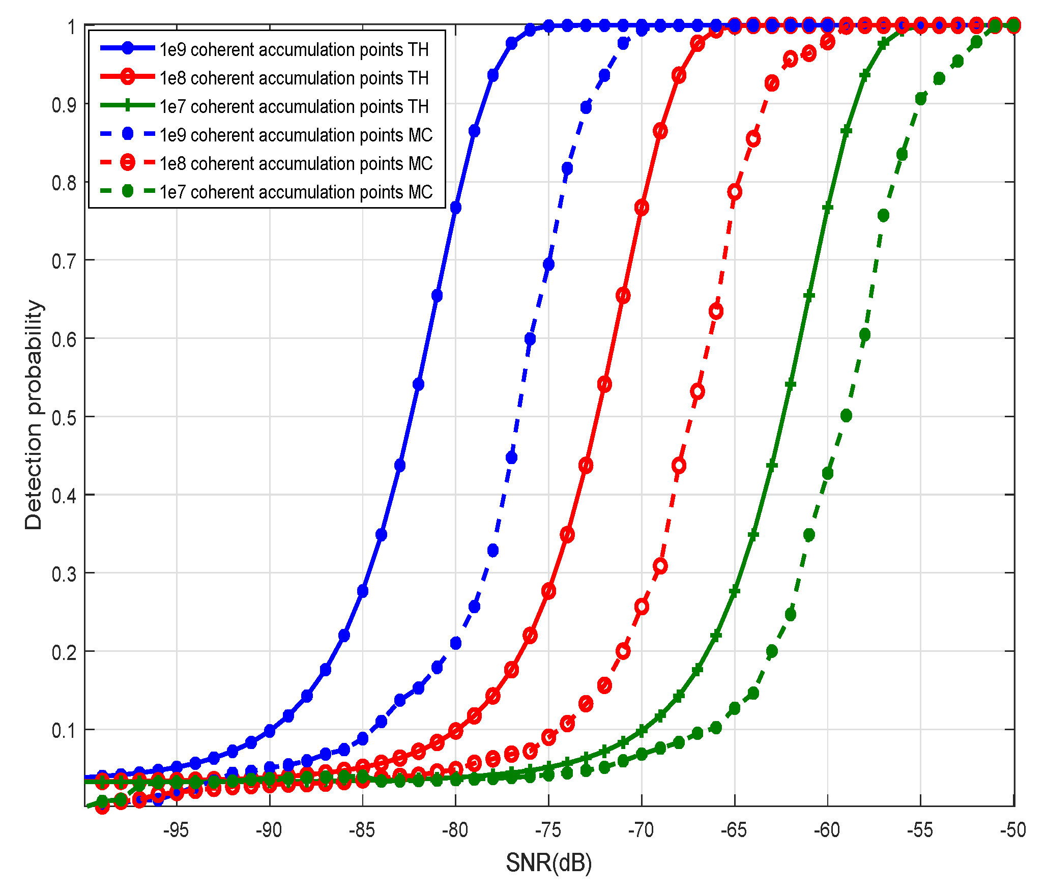
5.1. Performance Analysis of Detection Based on CAF

Suppose that the real and imaginary parts of Gaussian noise $n\left(t\right)$ and Gaussian noise $n^{\prime }\left(t\right)$ are distributed as $N(0,{\sigma }_n^2)$ and $N(0,{\sigma }_{n^{\prime }}^2)$, respectively. The separated reference signal and the echo signal from which the direct wave signal and multipath interference are suppressed in the surveillance channel are calculated CAF and discrete, which can be expressed as

$${\chi }_i(l{T}_s,f_d)={\displaystyle \sum _{m=0}^{N-1}}{x_i}^{\ast }(m{T}_s-l{T}_s)y\left(m{T}_s\right)e^{j2\pi f_{d}m{T}_s},$$

(32)

where $T_s$ represents the sample interval, N is the number of sampling points and $T_s$ stands for the sampling time, $N=T_F/\phantom{T_F{T}_s}{T}_s$. Equation (32) can also be expressed as

$$\begin{array}{cc}\hfill {\chi }_i(l,f_d)& ={\displaystyle \sum _{m=0}^{N-1}}{x_i}^{\ast }(m-l)y\left(m\right)e^{j2\pi f_{d}m}\hfill \\ \hfill & ={\displaystyle \sum _{m=0}^{N-1}}\mathrm{Re}\left\{y\left(m\right){x_i}^{\ast }(m-l)e^{j2\pi f_{d}m}\right\}+j{\displaystyle \sum _{m=0}^{N-1}}\mathrm{Im}\left\{y\left(m\right)x_i^{\ast }(m-l)e^{j2\pi f_{d}m}\right\}.\end{array}$$

(33)

Lemma 1.

The distribution of the detection based on CAF under the $H_1$ hypothesis is

$$(\mathsf{\Lambda }/H_1)\sim CN({r_i}^{\ast }{r}_i^{{}^{\prime }}{\chi }_{s_i{s}_i}(l-\zeta ,f_d-f_{d_i}),2N(r_i^2{\sigma }_{n^{\prime }}^2+{\displaystyle \sum _{\eta =1}^M}r{{}_{\eta }^{{}^{\prime }}}^2{\sigma }_n^2)),$$

(34)

and the distribution of the detection based on CAF under the $H_0$ hypothesis is

$$(\mathsf{\Lambda }/H_0)\sim CN(0,2N(r_i^2{\sigma }_{n^{\prime }}^2+{\displaystyle \sum _{\genfrac{}{}{0pt}{}{\eta =1\hfill }{\eta \ne i\hfill }}^M}{r}_{\eta }^{{}^{\prime }2}{\sigma }_n^2)),$$

(35)

where $CN(.)$ represents the complex Gaussian process.

Proof. 

See Appendix A.1. □

Form the above analysis, the detection probability of each sensor is

$$p_{d_i}={\int }_{T_{d_i}}^{+\infty }\rho (\mathsf{\Lambda }/H_1)d\mathsf{\Lambda }=Q_1\left(\sqrt{\frac{{\left|N{r}_i{r}_i^{{}^{\prime }}\right|}^2}{N(r_i^2{\sigma }_{n^{\prime }}^2+{\displaystyle \sum _{\eta =1}^M}{r^{{}^{\prime }}}_{\eta }^2{\sigma }_n^2)}},\sqrt{\frac{T_{d_i}}{N(r_i^2{\sigma }_{n^{\prime }}^2+{\displaystyle \sum _{\eta =1}^M}{r^{{}^{\prime }}}_{\eta }^2{\sigma }_n^2)}}\right),$$

(36)

where $\rho (\mathsf{\Lambda }/H_1)$ represents the probability density function of $(\mathsf{\Lambda }/H_1)$, $Q_1(·,·)$ denotes the Marcum Q function [26,27,28]. The false alarm probability for each sensor is

$$P_{f_i}={\int }_{T_{d_i}}^{+\infty }\rho (\mathsf{\Lambda }/H_0)d\mathsf{\Lambda }=exp\left(-\frac{T_{d_i}}{2N(r_i^2{\sigma }_{n^{\prime }}^2+{\displaystyle \sum _{\genfrac{}{}{0pt}{}{\eta =1\hfill }{\eta \ne i\hfill }}^M}{r}_{\eta }^{{}^{\prime }2}{\sigma }_n^2}\right),$$

(37)

where $\rho (\mathsf{\Lambda }/H_0)$ represents the probability density function of $(\mathsf{\Lambda }/H_0)$. Substituting Equation (36) and Equation (37) into Equation (30) and Equation (31), the overall detection probability and false alarm probability after decision fusion are

$$\begin{array}{c}{P}_d={\displaystyle \sum _{i^{\prime }=k}^h}{{\displaystyle \sum _{\sum u_i=i^{\prime }}}{\displaystyle \prod _i}\left\{\left(Q_1\left(\sqrt{\frac{{\left|N{r}_i{r}_i^{{}^{\prime }}\right|}^2}{N(r_i^2{\sigma }_{n^{\prime }}^2+{\displaystyle \sum _{\eta =1}^M}{\left(r_{\eta }^{{}^{\prime }}\right)}^2{\sigma }_n^2)}},\sqrt{\frac{T_{d_i}}{N(r_i^2{\sigma }_{n^{\prime }}^2+{\displaystyle \sum _{\eta =1}^M}{\left(r_{\eta }^{{}^{\prime }}\right)}^2{\sigma }_n^2)}}\right)\right)\right.}^{u_i}\hfill \\ {}_{}^{}{}_{}^{}{}_{}^{}{}_{}^{}{}_{}^{}{}_{}^{}{}_{}^{}{}_{}^{}{}_{}^{}\left.·{\left(1-Q_1\left(\sqrt{\frac{{\left|N{r}_i{r}_i^{{}^{\prime }}\right|}^2}{N(r_i^2{\sigma }_{n^{\prime }}^2+{\displaystyle \sum _{\eta =1}^M}{\left(r_{\eta }^{{}^{\prime }}\right)}^2{\sigma }_n^2)}},\sqrt{\frac{T_{d_i}}{N(r_i^2{\sigma }_{n^{\prime }}^2+{\displaystyle \sum _{\eta =1}^M}{\left(r_{\eta }^{{}^{\prime }}\right)}^2{\sigma }_n^2)}}\right)\right)}^{1-u_i}\right\},\hfill \end{array}$$

(38)

and

$$p_f={\displaystyle \sum _{i^{\prime }=k}^h}{\displaystyle \sum _{\sum u_i=i^{\prime }}}{\displaystyle \prod _i}exp{\left(-\frac{T_{d_i}}{2N(r_i^2{\sigma }_{n^{\prime }}^2+{\displaystyle \sum _{\genfrac{}{}{0pt}{}{\eta =1\hfill }{\eta \ne i\hfill }}^M}{r}_{\eta }^{{}^{\prime }2}{\sigma }_n^2}\right)}^{u_i}{\left(1-exp\left(-\frac{T_{d_i}}{2N(r_i^2{\sigma }_{n^{\prime }}^2+{\displaystyle \sum _{\genfrac{}{}{0pt}{}{\eta =1\hfill }{\eta \ne i\hfill }}^M}{r}_{\eta }^{{}^{\prime }2}{\sigma }_n^2}\right)\right)}^{1-u_i}.$$

(39)

The echo signal-to-noise ratio $SN{R}_{\eta }$ of the surveillance channel in the $\eta$-th detection channel is defined as

$$SN{R}_{\eta }=10lg\frac{{\left(r_{\eta }^{{}^{\prime }}\right)}^2}{{\sigma }_{n^{\prime }}^2}.$$

(40)

From Equation (40), we can obtain

$${10}^{\frac{SN{R}_{\eta }}{10}}=\frac{{\left(r_{\eta }^{{}^{\prime }}\right)}^2}{{\sigma }_{n^{\prime }}^2}.$$

(41)

In this case when $\eta$ is equal i, by substituting Equation (41) into Equation (36), we can get the relationship between the detection probability $p_{d_i}$ of a single sensor and the echo signal-to-noise ratio $SN{R}_i$ as

$$p_{d_i}\left(SN{R}_i\right)=Q_1\left(\frac{N\left|r_i{r}_i^{{}^{\prime }}\right|}{\sqrt{N(\frac{{r_i}^2{\left(r_i^{{}^{\prime }}\right)}^2}{{10}^{\frac{SN{R}_i}{10}}}+{\displaystyle \sum _{\eta =1}^M}{\left(r_{\eta }^{{}^{\prime }}\right)}^2{\sigma }_n^2)}},\frac{\sqrt{{T_d}_i}}{\sqrt{N(\frac{{r_i}^2{\left(r_i^{{}^{\prime }}\right)}^2}{{10}^{\frac{SN{R}_{s_i}}{10}}}+{\displaystyle \sum _{\eta =1}^M}{\left(r_{\eta }^{{}^{\prime }}\right)}^2{\sigma }_n^2)}}\right),$$

(42)

and the relationship between the final detection probability $p_d$ after the fusion and the echo signal-to-noise ratio $SNR$ is

$$\begin{array}{c}{p}_d={\displaystyle \sum _{i^{\prime }=k}^M}{\displaystyle \sum _{\sum u_i=i^{\prime }}}{\displaystyle \prod _{i=1}}{\left(Q_1\left(\sqrt{\frac{{\left|N{r}_i{r}_i^{{}^{\prime }}\right|}^2}{N(\frac{{r_i}^2{r_i^{\prime }}^2}{{10}^{\frac{SN{R}_i}{10}}}+{\displaystyle \sum _{\eta =1}^M}{r}_{\eta }^{{}^{\prime }2}{\sigma }_n^2)}},\sqrt{\frac{T_{d_i}}{N(\frac{{r_i}^2{r_i^{\prime }}^2}{{10}^{\frac{SN{R}_i}{10}}}+{\displaystyle \sum _{\eta =1}^M}{r}_{\eta }^{{}^{\prime }2}{\sigma }_n^2)}}\right)\right)}^{u_i}\hfill \\ ·{\left(1-Q_1\left(\sqrt{\frac{{\left|N{r}_i{r_i}^{{}^{\prime }}\right|}^2}{N(\frac{{r_i}^2{r_i^{\prime }}^2}{{10}^{\frac{SN{R}_i}{10}}}+{\displaystyle \sum _{\eta =1}^M}{r}_{\eta }^{{}^{\prime }2}{\sigma }_n^2)}},\sqrt{\frac{T_{d_i}}{N(\frac{{r_i}^2{r_i^{\prime }}^2}{{10}^{\frac{SN{R}_i}{10}}}+{\displaystyle \sum _{\eta =1}^M}{r}_{\eta }^{{}^{\prime }2}{\sigma }_n^2)}}\right)\right)}^{1-u_i}.\hfill \end{array}$$

(43)

From Equation (43), it can be seen that the detection probability $p_d$ is related to the number of sampling points N, the power ratio of the direct echo ${r_i}^2/\phantom{{r_i}^2{r_i^{\prime }}^2}{r_i^{\prime }}^2$, the detection threshold $T_{d_i}$ and the noise power ${\sigma }_n^2$ in the reference channel with different echo signal-to-noise $SN{R}_i$.

5.2. Performance Analysis of Detection Based on FOCCCAF

It is assumed that the noises $n\left(t\right)$ and $n^{{}^{\prime }}\left(t\right)$ obey the Gaussian distribution of $N(0,{\sigma }_n^2)$ and $N(0,{\sigma }_{n^{{}^{\prime }}}^2)$, respectively. We can get the FOCCCAF from the separated reference signal and the echo signal after the DPI and MPI suppression in the supervise channel by using Equation (10).

Lemma 2.

The distribution of the detection based on FOCCCAF under the $H_1$ hypothesis is

$$\begin{array}{c}\mathsf{\Lambda }/H_1\sim CN({r_i}^7{r_i}^{{}^{\prime }}{e}^{-j\pi ({\alpha }_i-f-f_{d_i})D_i}{\chi }_{4s_i}^{{\alpha }_i-f-f_{d_i},{\alpha }_i}(u,f)+9AB{r_i}^3{r_i}^{{}^{\prime }}{e}^{-j\pi ({\alpha }_i-f-f_{d_i})D_i}{\chi }_{2s_i}^{{\alpha }_i-f-f_{d_i},{\alpha }_i}(u,f),\hfill \\ \frac{{\sigma }_{s_i}^{10}}{N^3}(81A^2{r_i}^8{\left(r_i^{{}^{\prime }}\right)}^2{\sigma }_n^2+9{r_i}^{12}{\left(r_i^{{}^{\prime }}\right)}^2{\sigma }_n^2{\sigma }_{s_i}^4+9A^2{r_i}^{10}{\sigma }_{n^{{}^{\prime }}}^2+r_i^{14}{\sigma }_{n^{{}^{\prime }}}^2{\sigma }_{s_i}^4)).\hfill \end{array}$$

(44)

and the distribution of the detection based on FOCCCAF under the $H_0$ hypothesis is

$$\mathsf{\Lambda }/H_0\sim CN(0,\frac{{\sigma }_{s_i}^{10}}{N^3}({\displaystyle \sum _{\genfrac{}{}{0pt}{}{\eta =1\hfill }{\forall \eta \ne i\hfill }}^{M^{{}^{\prime }}}}81A^2{r}_i^8{\left(r_{\eta }^{{}^{\prime }}\right)}^2{\sigma }_n^2+{\displaystyle \sum _{\genfrac{}{}{0pt}{}{\eta =1\hfill }{\forall \eta \ne i\hfill }}^{M^{{}^{\prime }}}}9r_i^{12}{\left(r_{\eta }^{{}^{\prime }}\right)}^2{\sigma }_n^2{\sigma }_{s_i}^4+9A^2{r}_i^{10}{\sigma }_{n^{{}^{\prime }}}^2+r_i^{14}{\sigma }_{n^{{}^{\prime }}}^2{\sigma }_{s_i}^4)).$$

(45)

Proof. 

See Appendix A.2. □

From the above analysis, the detection probability for each sensor is

$$p_{d_i}={\int }_{T_{d_i}}^{+\infty }\rho (\mathsf{\Lambda }/H_1)d\mathsf{\Lambda }=Q_1\left(\sqrt{\frac{N^2{\left|{r_i}^7{r_i}^{{}^{\prime }}+9AB{r_i}^3{r_i}^{{}^{\prime }}\right|}^2}{Y}},\sqrt{\frac{T_{d_i}}{Y}}\right),$$

(46)

where $\rho (\mathsf{\Lambda }/H_1)$ represents the probability density function of $(\mathsf{\Lambda }/H_1)$ and $Y=\frac{{\sigma }_{s_i}^{10}}{N^3}(81A^2{r}_i^8{\left(r_i^{{}^{\prime }}\right)}^2{\sigma }_n^2+9r_i^{12}{\left(r_i^{{}^{\prime }}\right)}^2{\sigma }_n^2{\sigma }_{s_i}^4+9A^2{r}_i^{10}{\sigma }_{n^{{}^{\prime }}}^2+r_i^{14}{\sigma }_{n^{{}^{\prime }}}^2{\sigma }_{s_i}^4)$. The false alarm probability for each sensor is

$$\begin{array}{c}{P}_{f_i}={\int }_{T_{d_i}}^{+\infty }\rho (\mathsf{\Lambda }/H_0)d\mathsf{\Lambda }\hfill \\ =exp\left(-\frac{T_{d_i}}{\frac{{\sigma }_{s_i}^{10}}{N^3}({\displaystyle \sum _{\genfrac{}{}{0pt}{}{\eta =1\hfill }{\forall \eta \ne i\hfill }}^{M^{{}^{\prime }}}}81A^2{r}_i^8{\left(r_{\eta }^{{}^{\prime }}\right)}^2{\sigma }_n^2+{\displaystyle \sum _{\genfrac{}{}{0pt}{}{\eta =1\hfill }{\forall \eta \ne i\hfill }}^{M^{{}^{\prime }}}}9r_i^{12}{\left(r_{\eta }^{{}^{\prime }}\right)}^2{\sigma }_n^2{\sigma }_{s_i}^4+9A^2{r}_i^{10}{\sigma }_{n^{{}^{\prime }}}^2+r_i^{14}{\sigma }_{n^{{}^{\prime }}}^2{\sigma }_{s_i}^4)}\right),\hfill \end{array}$$

(47)

where $\rho (\mathsf{\Lambda }/H_0)$ represents the probability density function of $(\mathsf{\Lambda }/H_0)$. Substituting Equation (46) and Equation (47) into Equation (30) and Equation (31), the detection probability and false alarm probability after distributed sensor fusion are

$$\begin{array}{c}{P}_d={\displaystyle \sum _{i^{\prime }=k}^h}{\displaystyle \sum _{\sum u_i=i^{\prime }}}{\displaystyle \prod _i}{\left(Q_1\left(\sqrt{\frac{N^2{\left|{r_i}^7{r_i}^{{}^{\prime }}+9AB{r_i}^3{r_i}^{{}^{\prime }}\right|}^2}{Y}},\sqrt{\frac{T_{d_i}}{Y}}\right)\right)}^{u_i}\hfill \\ ·{\left(1-Q_1\left(\sqrt{\frac{N^2{\left|r_i^7{r_i}^{{}^{\prime }}+9AB{r_i}^3{r_i}^{{}^{\prime }}\right|}^2}{Y}},\sqrt{\frac{T_{d_i}}{Y}}\right)\right)}^{1-u_i},\hfill \end{array}$$

(48)

and

$$p_f={\displaystyle \sum _{i^{\prime }=k}^h}{\displaystyle \sum _{\sum u_i=i^{\prime }}}{\displaystyle \prod _i}exp{(-\frac{T_{d_i}}{\mathsf{\Delta }})}^{u_i}{(1-exp(-\frac{T_{d_i}}{\mathsf{\Delta }}))}^{1-u_i},$$

(49)

where $\mathsf{\Delta }=\frac{{\sigma }_{s_i}^{10}}{N^3}({\displaystyle \sum _{\genfrac{}{}{0pt}{}{\eta =1\hfill }{\forall \eta \ne i\hfill }}^{M^{{}^{\prime }}}}81A^2{r}_i^8{\left(r_{\eta }^{{}^{\prime }}\right)}^2{\sigma }_n^2+{\displaystyle \sum _{\genfrac{}{}{0pt}{}{\eta =1\hfill }{\forall \eta \ne i\hfill }}^{M^{{}^{\prime }}}}9r_i^{12}{\left(r_{\eta }^{{}^{\prime }}\right)}^2{\sigma }_n^2{\sigma }_{s_i}^4+9A^2{r}_i^{10}{\sigma }_{n^{{}^{\prime }}}^2+r_i^{14}{\sigma }_{n^{{}^{\prime }}}^2{\sigma }_{s_i}^4)$. In the supervise channel, the $i_{th}(i=\eta )$ echo signal-to-noise ratio $SN{R}_i$ is defined as

$$SN{R}_i=10lg\frac{{\left(r_i^{{}^{\prime }}\right)}^2}{{\sigma }_{n{}^{\prime }}^2}.$$

(50)

From Equation (50), we can obtain

$${10}^{\frac{SN{R}_i}{10}}=\frac{{\left(r_i^{{}^{\prime }}\right)}^2}{{\sigma }_{n{}^{\prime }}^2}.$$

(51)

Substituting Equation (51) into Equation (46), the relationship between the detection probability of a single sensor $P_{d_i}$ and the echo signal-to-noise ratio $SN{R}_i$ is expressed as follows

$$p_{d_i}={\int }_{T_{d_i}}^{+\infty }\rho (\mathsf{\Lambda }/H_1)d\mathsf{\Lambda }=Q_1\left(\sqrt{\frac{N^2{\left|r_i^7{r_i}^{{}^{\prime }}+9AB{r_i}^3{r_i}^{{}^{\prime }}\right|}^2}{\mathsf{\Xi }}},\sqrt{\frac{T_{d_i}}{\mathsf{\Xi }}}\right),$$

(52)

where $\mathsf{\Xi }=\frac{{\sigma }_{s_i}^{10}}{N^3}(81A^2{r}_i^8{\left(r_i^{{}^{\prime }}\right)}^2{\sigma }_n^2+9r_i^{12}{\left(r_i^{{}^{\prime }}\right)}^2{\sigma }_n^2{\sigma }_{s_i}^4+9A^2{r}_i^{10}\frac{9A^2{r}_i^{10}{\left(r_i^{{}^{\prime }}\right)}^2}{{10}^{\frac{SN{R}_i}{10}}}+r_i^{14}\frac{{\left(r_i^{{}^{\prime }}\right)}^2}{{10}^{\frac{SN{R}_i}{10}}}{\sigma }_{s_i}^4)$. The relationship between the final detection probability after fusion $P_d$ and the echo signal-to-noise ratio SNR is expressed as follows:

$$\begin{array}{c}{P}_d={\displaystyle \sum _{i^{\prime }=k}^h}{\displaystyle \sum _{\sum u_i=i^{\prime }}}{\displaystyle \prod _i}{\left(Q_1\left(\sqrt{\frac{N^2{\left|r_i^7{r_i}^{{}^{\prime }}+9AB{r_i}^3{r_i}^{{}^{\prime }}\right|}^2}{\mathsf{\Xi }}},\sqrt{\frac{T_{d_i}}{\mathsf{\Xi }}}\right)\right)}^{u_i}\hfill \\ ·{\left(1-Q_1\left(\sqrt{\frac{N^2{\left|{r_i}^7{r_i}^{{}^{\prime }}+9AB{r_i}^3{r_i}^{{}^{\prime }}\right|}^2}{\mathsf{\Xi }}},\sqrt{\frac{T_{d_i}}{\mathsf{\Xi }}}\right)\right)}^{1-u_i}.\hfill \end{array}$$

(53)

From Equation (53), it can be seen that the detection probability $P_d$ is related to the number of sampling points N and the power ratio of the direct echo $r_i^2/\phantom{r_i^{2}r{{}_i^{{}^{\prime }}}^2}r{{}_i^{{}^{\prime }}}^2$, the power of $s_i\left(t\right)$ and the noise power in the reference channel with different echo signal-to-noise.

6. Numerical Results and Discussion

To verify the effectiveness of the proposed passive detection method and investigate and the influence of different parameters on the detection performance, a series of simulation experiments are conducted using MATLAB (9.5.0.944444 (R2018b), MathWorks Company, Natick, MA, USA). Simulation parameters are set according to [29,30]. GPS satellite, DVB-S satellite and INMARSAT satellite signals are considered in the simulation with Gaussian white noise. The ratio of echo signal to direct wave power is defined as

$$DSR=\frac{P_D}{P_S},$$

(54)

where N represents the number of sampling points, $P_S$ and $P_D$ are the power of the direct wave and the echo, respectively. The detection accuracy rate is used to evaluate the detection algorithm as

$${\delta }_H=\frac{N_R}{N}\times 100\%,$$

(55)

where ${\delta }_H$ and $N_R$ are the number of corrected detection and the total number of detection in the simulation, respectively.

In order to evaluate the influence of sampling points on the detection performance of weak echo signals, three satellite signals GPS, DVB-S and INMARSAT are used for simulation experiments. The carrier frequencies of the three signals are: 1.57 GHz, 12.38 GHz, 4.2 GHz; the chip-rates are: 1.023 MHz, 22.425 MHz, 2.2 MHz; the delay is 1 us, 2 us, 3 us; the doppler shift are: 100 Hz, 200 Hz, 300 Hz; the intensity of the three signal direct waves are: −130.1 dBw, −111.83 dBw, −120.61 dBw, and the direct wave and its corresponding echo power difference are 40 dBw, $P_{fa}={10}^{-4}$, coherent accumulation points are: ${10}^7$, ${10}^8$, ${10}^9$.2000 Monte Carlo simulation experiments are carried out and the simulation results are shown in Figure 4.

From Figure 4, it can be seen that the detection performance of the weak echo gradually increases with the increase of the accumulated points under the same SNR. This is because, as the number of accumulated points increases, the peaks at the corresponding delay and Doppler frequency shift become more prominent, which is equivalent to increasing the echo SNR gain, thereby improving detection performance. When the cumulative number of points is ${10}^9$ and the SNR is −75 dB, the detection probability of the echo signal reaches 99%. For the same cumulative number of points, as the SNR becomes larger, the detection performance improves. The simulation results agree with the theoretical results, and the feasibility of detecting weak echo signals based on FOCCCAF is verified.

In order to compare the proposed method based on FOCCCAF with the method based on CAF, three satellite signals GPS, DVB-S and INMARSAT satellite signals are used for simulation experiments. $P_{fa}={10}^{-4}$, coherent accumulation point is ${10}^9$, 2000 Monte Carlo simulation experiments are carried out and the simulation results are shown in Figure 5.

It can be seen from Figure 5 that the detection performance based on FOCCCAF is better than that on CAF, and the detection performance is improved by about 6 dB. This is because both FOCCCAF and CAF perform echo detection by detecting the delay of the corresponding echo signal and the peak at the Doppler shift, and the fourth-order cyclic cumulant can suppress noise, which is equivalent to increasing the detected peak value, so that the FOCCCAF-based peak under the same echo SNR is more prominent, which is beneficial to the detection of echo signals. The theoretical and actual detection performance are consistent, verifying the superiority of FOCCCAF-based detection performance to CAF.

In order to verify the impact of false alarm probability on the performance of the proposed method, the detection performance of the method under different false alarm probabilities is simulated. GPS, DVB-S and INMARSAT satellite signals are used for simulation experiments. coherent accumulation point is ${10}^9$, 2000 Monte Carlo simulation experiments are carried out and the simulation results are shown in Figure 6.

From Figure 6, it can be seen that, under the same SNR, the greater the false alarm probability, the greater the detection probability. The simulation gives the relationship between the echo SNR and the detection probability of the false alarm probability at ${10}^{-4}$, ${10}^{-5}$ and ${10}^{-6}$. When the echo SNR is around −75 dB and the accumulated point reaches ${10}^9$, the detection probability of the echo signal reaches 1. When the echo SNR is −95 dB, the detection probability is 0. This is because the echo SNR is too low, even if the accumulated points reach ${10}^9$, the detected peak cannot be highlighted. To detect weak echo signals at this SNR, we need more points to accumulate.

In order to verify the impact of SDR on detection performance, GPS, DVB-S and INMARSAT satellite signals are used for simulation experiments. $P_{fa}={10}^{-4}$, coherent accumulation point is ${10}^9$, 2000 Monte Carlo simulation experiments are carried out and the simulation results are shown in Figure 7.

In order to verify the impact of SDR on detection performance, GPS, DVB-S and INMARSAT satellite signals are used for simulation experiments. $P_{fa}={10}^{-4}$, coherent accumulation point is ${10}^9$, 2000 Monte Carlo simulation experiments are carried out and the simulation results are shown in Figure 7.

It can be seen from Figure 7 that the detection performance of the echo signal is becoming better and better with the increase of the echo direct wave power ratio. This is because under the condition that the direct wave power is constant, as the echo direct wave power ratio increases, the echo signal is enhanced, and the detected peak can be highlighted. This is equivalent to improving the SNR, so the detection of echo signals is promoted. The correctness of the theory is verified by actual simulation.

In order to compare the detection performance with different methods, GPS, DVB-S and INMARSAT satellite signals are used for simulation experiments. $P_{fa}={10}^{-4}$, coherent accumulation point is ${10}^9$, 2000 Monte Carlo simulation experiments are carried out and the simulation results are shown in Figure 8. From Figure 8, it can be seen that under the same conditions, the detection probability based on FOCCCAF which is proposed in this paper is better than that of CAF and CCAF in [16].

7. Conclusions

In this paper, a novel method of the passibe moving aerial target detection has been proposed under collaborative heterogeneous multiple satellites, in which parallel band-pass filters and an NLMS-based adaptive filter based on NLMS are used to separate direct wave signals in the reference channel and suppress DPI/MPI in the surveillance channel, respectively. Then, the detection statistic of weak echo signals from multiple heterogeneous satellites was obtained by using the anti-interference property of FOOCCCAF. Through distributed multi-sensors fusion, multiple detection results have been superimposed to obtain final detection results. Finally, depending on the theoretical analysis of the detection statistics, the relationship between the detection performance and a series of key parameters is studied. Numerical results have demonstarted that the proposed method is able to precisely detect a moving target in multiple heterogeneous satellite environments. This indicated that in a complicated environment with multiple satellites, the proposed method is more applicable than the methods relying on a single satellite as the illumination for passive detection.

References

1. Hashim, I.; Al-Hourani, A.; Rowe, W.; Scott, J. Adaptive X-Band Satellite Antenna for Internet-of-Things (IoT) over Satellite Applications. In Proceedings of the 13th International Conference on Signal Processing and Communication Systems, Surfers Paradise, Australia, 16–18 December 2019; pp. 1–7. [Google Scholar]
2. Li, F.; Lam, K.; Zhao, N.; Liu, X.; Zhao, K.; Wang, L. Spectrum Trading for Satellite Communication Systems with Dynamic Bargaining. IEEE Trans. Commun. 2018, 66, 4680–4693. [Google Scholar] [CrossRef]
3. Ilyushin, Y.; Padokhin, A.; Smolov, V. Global Navigational Satellite System Phase Altimetry of the Sea Level: Systematic Bias Effect Caused by Sea Surface Waves. In Proceedings of the 2019 PhotonIcs & Electromagnetics Research Symposium—Spring (PIERS-Spring), Rome, Italy, 17–20 June 2019; pp. 1618–1627. [Google Scholar]
4. Qiao, J.; Chen, W.; Ji, S.; Weng, D. Accurate and Rapid Broadcast Ephemerides for Beidou-Maneuvered Satellites. Remote. Sens. 2019, 11, 787. [Google Scholar] [CrossRef] [Green Version]
5. Powell, S.; Akos, D. GNSS Reflectrometry Using the L5 and E5a Signals for Remote Sensing Applications. In Proceedings of the 2013 US National Committee of URSI National Radio Science Meeting, Boulder, CO, USA, 9–12 January 2013; p. 1. [Google Scholar]
6. Clarizia, M.; Chotiros, N.; Vaccaro, M. A GPS-Reflectometry Simulator for Target Detection Over Oceans. In Proceedings of the IGARSS 2018–2018 IEEE International Geoscience and Remote Sensing Symposium, Valencia, Spain, 23–27 July 2018; pp. 450–451. [Google Scholar]
7. Garvanov, I.; Kabakchiev, C.; Behar, V.; Garvanova, M. Target Detection Using a GPS Forward-Scattering Radar. In Proceedings of the 2015 International Conference on Engineering and Telecommunication, Mosocw, Russia, 18–19 November 2015; pp. 29–33. [Google Scholar]
8. Clarizia, M.; Braca, P.; Ruf, C.S.; Willett, P. Target Detection Using GPS Signals of Opportunity. In Proceedings of the 2015 18th International Conference on Information Fusion, Washington, DC, USA, 6–9 July 2015; pp. 1429–1436. [Google Scholar]
9. Gronowski, K.; Samczynski, P.; Stasiak, K.; Kulpa, K. First, Results of Air Target Detection Using Single Channel Passive Radar Utilizing GPS Illumination. In Proceedings of the 2019 IEEE Radar Conference, Boston, MA, USA, 22–26 April 2019; pp. 1–6. [Google Scholar]
10. Mojarrabi, B.; Homer, J.; Kubik, K. Power Budget Study for Passive Target Detection and Imaging Using Secondary Applications of GPS Signals in Bistatic Radar Systems. In Proceedings of the IEEE International Geoscience and Remote Sensing Symposium, Toronto, ON, Canada, 24–28 June 2002; pp. 449–451. [Google Scholar]
11. Zeng, H.; Chen, J.; Wang, P.; Yang, W.; Liu, W. 2D Coherent Integration Processing and Detecting of Aircrafts Using GNSS-Based Passive Radar. Remote. Sens. 2018, 10, 1164. [Google Scholar] [CrossRef] [Green Version]
12. AlJewari, Y.; Ahmad, R.; AlRawi, A. Impact of Multipath Interference and Change of Velocity on the Reliability and Precision of GPS. In Proceedings of the 2014 2nd International Conference on Electronic Design, Penang, Malaysia, 19–21 August 2014; pp. 427–430. [Google Scholar]
13. Wu, X.; Gong, P.; Zhou, J.; Liu, Z. The Applied Research on Anti-multipath Interference GPS Signal Based on Narrow-related. In Proceedings of the 2014 IEEE 5th International Conference on Software Engineering and Service Science, Beijing, China, 27–29 June 2014; pp. 771–774. [Google Scholar]
14. Suberviola, I.; Mayordomo, I.; Mendizabal, J. Experimental Results of Air Target Detection with a GPS Forward-Scattering Radar. IEEE Geosci. Remote Sens. Lett. 2011, 9, 47–51. [Google Scholar] [CrossRef]
15. Lashley, M.; Bevly, D.; Hung, J. Performance Analysis of Vector Tracking Algorithms for Weak GPS Signals in High Dynamics. IEEE J. Sel. Top. Signal Process. 2009, 3, 661–673. [Google Scholar] [CrossRef]
16. Liu, M.; Gao, Z.; Chen, Y.; Song, H.; Li, Y.; Gong, F. Passive Detection of Moving Aerial Target Based on Multiple Collaborative GPS Satellites. Remote. Sens. 2020, 12, 263. [Google Scholar] [CrossRef] [Green Version]
17. Liu, M.; Yi, F.; Liu, P.; Li, B. Cramer-Rao Lower Bounds of TDOA and FDOA Estimation Based on Satellite Signals. In Proceedings of the 2018 14th IEEE International Conference on Signal Processing, Beijing, China, 12–16 August 2018; pp. 1–4. [Google Scholar]
18. Masjedi, S.; Moddares-Hashemi, M. Theoretical Approach for Target Detectionand Interference Cancellation in Passive Radar. IET Radar Sonar Navig. 2013, 7, 205–216. [Google Scholar] [CrossRef]
19. Zhang, Y.; Xi, S. Application of New LMS Adaptive Filtering Algorithm with Variable Step Size in Adaptive Echo Cancellation. In Proceedings of the 2017 IEEE 17th International Conference on Communication Technology, Chengdu, China, 27–30 October 2017; pp. 1715–1719. [Google Scholar]
20. Niranjan, D.; Ashwini, B. Noise Cancellation in Musical Signals Using Adaptive Filtering Algorithms. In Proceedings of the 2017 International Conference on Innovative Mechanisms for Industry Applications, Bangalore, India, 21–23 February 2017; pp. 82–86. [Google Scholar]
21. Mugdha, A.; Rawnaque, F.; Ahmed, M. A Study of Recursive Least Squares (RLS) Adaptive Filter Algorithm in Noise Removal from ECG Signals. In Proceedings of the 2015 International Conference on Informatics, Electronics Vision, Fukuoka, Japan, 15–18 June 2015; pp. 1–6. [Google Scholar]
22. Cardinali, R.; Colone, F.; Ferretti, C.; Lombardo, P. Comparison of Clutter and Multipath Cancellation Techniques for passive Radar. In Proceedings of the 2007 IEEE Radar Conference, Boston, MA, USA, 17–20 April 2007; pp. 469–474. [Google Scholar]
23. Liu, M.; Zhang, J.; Li, B. Feasibility Analysis of OFDM/OQAM Signals as Illuminator of Opportunity for Passive Detection. In Proceedings of the 2018 14th IEEE International Conference on Signal Processing, Beijing, China, 12–16 August 2018; pp. 1–4. [Google Scholar]
24. Hong, J.; Wang, S.X.; Lu, H.J. An Effective Direction Estimation Algorithm in Multipath Environment Based on Fourth-order Cyclic Cumulants. In Proceedings of the IEEE 5th Workshop on Signal Processing Advances in Wireless Communications, Lisbon, Portugal, 11–14 July 2004; pp. 263–267. [Google Scholar]
25. Yan, X.; Wang, S.; Wang, K.; Jiang, H. Localization of Near field Cyclostationary Source Based on Fourth-order Cyclic Cumulant. In Proceedings of the 2008 9th International Conference on Signal Processing, Beijing, China, 26–29 October 2008; pp. 1629–1632. [Google Scholar]
26. Jun, H. A proper integral representation of Marcum Q-Function. In Proceedings of the 2014 XXXIth URSI General Assembly and Scientific Symposium, Beijing, China, 16–23 August 2014; pp. 1–3. [Google Scholar]
27. Bocus, M.; Dettmann, C.; Coon, J. An Approximation of the First Order Marcum Q-Function with Application to Network Connectivity Analysis. IEEE Commun. Lett. 2013, 17, 499–502. [Google Scholar] [CrossRef] [Green Version]
28. Ermolova, N.; Tirkkonen, O. Laplace Transform of Product of Generalized Marcum Q, Bessel I, and Power Functions With Applications. IEEE Trans. Signal Process. 2014, 62, 2938–2944. [Google Scholar]
29. Hu, B.; Liu, M.; Yi, F.; Song, H.; Jiang, F.; Gong, F.; Zhao, N. DOA Robust Estimation of Echo Signals Based on Deep Learning Networks with Multiple Type Illuminators of Opportunity. IEEE Access 2020, 8, 14809–14819. [Google Scholar] [CrossRef]
30. Liu, M.; Zhang, J.; Tang, J.; Jiang, F.; Liu, P.; Gong, F.; Zhao, N. 2D DOA Robust Estimation of Echo Signals Based on Multiple Satellites Passive Radar in the Presence of Alpha Stable Distribution Noise. IEEE Access 2019, 7, 2169–3536. [Google Scholar]
Figure 1. Passive detection system model based on multiple collaborative heterogeneous satellites.
Remotesensing 12 01150 g001
Figure 2. Spectrogram of three time-domain overlapped satellite signals.
Remotesensing 12 01150 g002
Figure 3. Spectrograms of three time-domain overlapped satellite signals after separation. (a) Spectrogram of GPS satellite signal; (b) Spectrogram of INMARSAT satellite signal; (c) Spectrogram of DVB-S satellite signal.
Remotesensing 12 01150 g003
Figure 4. Relationship between coherent accumulation points and detection performance.
Remotesensing 12 01150 g004
Figure 5. Detection performance of the proposed method.
Remotesensing 12 01150 g005
Figure 6. Detection performance with different false alarm probabilities.
Remotesensing 12 01150 g006
Figure 7. Relationship between SDR and detection performance.
Remotesensing 12 01150 g007
Figure 8. Detection performance comparison with different methods.
Remotesensing 12 01150 g008