Abstract
Mapping and monitoring agricultural land-use intensity (LUI) changes are essential for understanding their effects on biodiversity. Current land-use models provide a rather coarse spatial resolution, while in-situ measurements of LUI cover only a limited extent and are time-consuming and expensive. The purpose of this study is to evaluate the feasibility of using habitat type, topo-climatic, economic output, and remote-sensing data to map LUI at a high spatial resolution. To accomplish this, we first rated the habitat types across the agricultural landscape in terms of the amount and frequency of fertiliser input, pesticide input, ploughing, grazing, mowing, harvesting, and biomass output. We consolidated these ratings into one LUI index per habitat type that we then related to topo-climatic, economic output, and remote-sensing predictors. The results showed that the LUI index was strongly related to plant indicator values for mowing tolerance and soil nutrient content and to aerial nitrogen deposition, and thus, is an adequate index. Topo-climatic, and, to a smaller extent, economic output and remote-sensing predictors, proved suitable for mapping LUI. Large- to medium-scale patterns are explained by topo-climatic predictors, while economic output predictors explain medium-scale patterns and remote-sensing predictors explain local-scale patterns. With the fine-scale LUI map produced from this study, it is now possible to estimate within unvarying land-use classes, the effect on agrobiodiversity of an increase in LUI on fertile and accessible lands and of a decrease of LUI by the abandonment of marginal agricultural lands, and thus, provide a valuable base for understanding the effects of LUI on biodiversity. Due to the worldwide availability of remote-sensing and climate data, our methodology can be easily applied to other countries where habitat-type data are available. Given their low explanatory power, economic output variables may be omitted if not available.
1. Introduction
Future growth in human population and prosperity will increase the demand for food and fuel [1]. Meeting this demand will require changes in agricultural land use [2]. Agricultural land-use change impacts biodiversity and therefore ecosystem services [3,4,5]. Biodiversity loss from agricultural land-use change occurs due to changes in landscape composition (i.e., proportion of cultivated land), landscape configuration (i.e., spatial arrangement of landscape elements), and land-use intensity (LUI) (i.e., number of inputs and outputs) [5,6,7,8]. In western Europe, land resources that are suitable for agricultural cultivation are becoming scarce, and thus, there are limited opportunities for increasing the proportion of cultivated land without very high costs, which are economically not profitable [9]. Therefore, changes in LUI are most important [8].
Land-use intensification involves the introduction of high-input arable systems on fertile and accessible lands, along with the abandonment of marginal agricultural lands [10,11]. This leads to the loss of semi-natural areas [12], to an increase in habitat fragmentation [8], to an alteration of habitat types [13], and to natural succession on marginal land [14,15]. Yet, land-use science has mainly focused on broad land-cover conversions, while spatial patterns in LUI within cropland, grazing, and mowing systems remain highly unclear [16,17,18]. Furthermore, studies that assess the effect of LUI on biodiversity assume that intensively used agricultural land, which surrounds semi-natural habitats, is entirely unsuitable for most species, based on the island biogeography theory. These studies measure LUI as the area of, or distance to, semi-natural habitats such as woody elements [19,20,21,22]; the percentage of permanent grassland [23]; the percentage of arable fields [24]; or broad habitat classes [25]. However, it is now acknowledged that intensively used agricultural land may not always be entirely unsuitable [26,27,28]. Some agricultural resources have positive consequences for species’ persistence, dispersal, and colonisation [29,30,31]. The failure to address LUI more precisely has limited scientists’ ability to make credible evaluations of the impacts of changes in land use and land cover on biodiversity in a changing climate [17,32]. A finely graduated index with a high spatial resolution may provide vital information on the effects of LUI on biodiversity.
To map LUI with a high spatial resolution, LUI has to be first parametrised and then spatialised. LUI can be parametrised by defining it as the combined effect of agricultural inputs (e.g., fertiliser, pesticide, ploughing) and biomass outputs (e.g., grazing, mowing, harvest) [33,34]. These components of LUI are currently spatialised by remote-sensing approaches, land-use models, and farmer interviews. Remote-sensing approaches primarily map LUI components by analysing temporal profiles of vegetation indices [35,36]. Before the launch of Sentinel satellites, remote-sensing approaches were mainly based on moderate resolution imaging spectroradiometer (MODIS; [35,37]), and thus had a rather low spatial resolution. In recent years, several studies have been developed that either use Sentinel-2 [38,39], or Sentinel-1 and Sentinel-2 combined [40,41]. Overall, remote-sensing approaches mostly focus on individual agricultural land-use classes (e.g., field crops [40], grassland [36]), or a few LUI components (e.g., biomass removal [42] or grassland mowing frequency [39]), without including ancillary predictors such as climate or topography, despite the fact that patterns on regional and global scales may strongly be topo-climatically determined. Current land-use models provide a detailed picture of the dynamics of land use [43], but the maps’ spatial resolution is too low for biodiversity analyses. Spatially explicit information for individual pieces of land from elaborate, detailed interviews with farmers [44,45] are very costly to compile and can be unreliable. Because land-use activities take place in production systems that are defined by their biophysical and economic properties [16], a new approach based on spatially explicit habitat-type data, topo-climatic data, economic output data, and remote-sensing data may help map LUI at a higher spatial resolution.
In the new approach, LUI parameters are derived from habitat types, i.e., areas with particular environmental conditions and management regimes that are sufficiently uniform to support a characteristic assemblage of organisms. Habitat type-specific ratings of agricultural inputs and biomass outputs are then assembled into an LUI index that can be spatialised. This spatialization is done by topo-climatic data that characterise the biophysical properties, economic output data that describe the economic properties, and remote-sensing data that address the actual local agricultural management, i.e., agricultural input and biomass output, which are constrained by the biophysical and economic properties.
In this paper, we (1) evaluate the feasibility of creating an LUI index by rating the agricultural inputs and biomass outputs per habitat type, (2) evaluate the feasibility of mapping this LUI index at a high spatial resolution by using topo-climatic data, economic output data, and remote-sensing data, and (3) evaluate the relative importance of the three predictor sets for determining LUI.
2. Materials and Methods
2.1. Framework
We selected the agricultural area of Switzerland as the study area. First, we created an expert-based LUI index for all 96 habitat types that typically occur in the agricultural landscape of Switzerland, as shown in Figure 1. We used a combined index of input and output, since these two dimensions of the LUI are not independent of each other. For example, fertiliser applications are often required to allow for higher mowing frequencies [46]. We evaluated the LUI index by correlating it to plant indicator values for mowing tolerance and soil nutrient content based on the plant communities from Switzerland’s farmland species and habitat monitoring program (ALL-EMA). Additionally, we compared the LUI index of these plots to the aerial nitrogen deposition map, which indicates different aspects of livestock breeding (housing, storage, and application of manure, grazing) and plant production (mineral fertilisers on cropland, grassland, and alpine pastures). To create the LUI maps, we spatially predicted the LUI index assigned to each ALL-EMA plot with the help of topo-climatic predictors (i.e., climate, topography, and soil), economic output predictors (i.e., agricultural standard outputs) and remote-sensing predictors (i.e., Normalised Difference Vegetation Index) based on data from Sentinel-2 sensors. Further, we estimated the relative importance of the three predictor sets for determining LUI using a variation partitioning analysis.
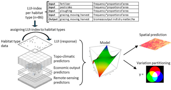
Figure 1.
Framework for creating, predicting, and evaluating a land-use intensity (LUI) index.
2.2. Study Area
The study area was located in and along the central Alps in Switzerland (45°49′N–47°48′N, 5°57′E–10°29′E; ~41,000 km2). North of the Alps, the climate is moist and maritime. The climate is drier and more continental in the interior Alpine valleys, and the southern climate is mild and humid. The Alps act as a barrier that separates the climates of the Mediterranean and central Europe. The study area is the agricultural landscape and encompasses approximately 15,000 km2 (Figure 2).
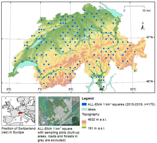
Figure 2.
Location of study area showing the 170 landscape squares of Switzerland’s farmland species and habitat monitoring program ALL-EMA (blue squares) and the farmland species and habitat monitoring plots within the agricultural landscape on a 50 m mesh (yellow dots).
2.3. Data
2.3.1. Habitat Types, Plant Species, and Plant Indicator Values
Data on habitat types and vascular plant species originated from Switzerland’s farmland species and habitat monitoring program (ALL-EMA; www.allema.ch). ALL-EMA performs surveys every five years on a given plot; the first five-year cycle started in 2015. Data are collected within the open agrarian landscape in 170 1 km2 landscape squares distributed across Switzerland (Figure 2). Habitat-type data were collected from circular plots with a size of 10 m2 located on a regular grid of 50 m. Forest, settlement, water bodies, glaciers, and rocks within the squares were not sampled. Data on vascular plants were obtained from a subsample of 19 plots. For the years 2015–2019, habitat-type information was available for 30,560 plots, and 3050 plots had a complete survey of vascular plants.
Plant indicator values for mowing tolerance and soil nutrient content are derived from Landolt et al. [47]. Mowing tolerance indicates the tolerance to a certain frequency of mowing or grazing. Soil nutrient content indicates the amount of available nitrogen and phosphorous in the soil. Indicator values range from 1 to 5. Low values indicate low mowing tolerance or low soil nutrient content, and high values indicate high mowing tolerance or high soil nutrient content. For each of the 3050 plots where we had a complete survey of vascular plants, mean indicator values were derived by calculating a plant cover [48] weighted mean of the indicator values.
2.3.2. Topo-Climatic, Economic, and Remote-Sensing Data
Topo-climatic, economic, and remote-sensing variables were selected based on their relevance to agricultural land use, plant physiology, and explaining spatial patterns. In total, 14 variables were selected (Table 1), which had a |rs| < 0.7 [49] and a Variance Inflation Factor < 5 [50,51] to reduce multicollinearity problems. All variables were generated with R [52] and ArcGIS 10.3 [53] and resampled to a 10 m spatial resolution.

Table 1.
Overview of the topo-climatic, economic, and remote-sensing variables and the nitrogen deposition data.
In terms of topo-climatic variables, we selected topographic, climatic, and edaphic variables. The topographic variables used are slope (°), potential yearly global radiation (kJ m−2 d−1), and topographical position index (m), which were all computed from a 25 × 25 m digital elevation model [54]. For climatic variables, we selected annual degree-days using a 0 °C threshold (°C d), summer frost days (d), and yearly precipitation days (d), which were all calculated from downscaled monthly temperature and precipitation maps (reference period 1950–2000) [55,56,57]. We selected soil suitability for agricultural land-use as an edaphic variable (soil suitability map of Switzerland [58]).
Standard output coefficients for Swiss agriculture describe the average monetary value of agricultural production at producer prices. We used average standard output coefficients for animal and crop production for 2005–2009 from the AGIS database [59]: cattle, sheep, and goats (AGIS-codes 1110–1586 and 1882); pigs and poultry (AGIS-codes 1611–1881); crop area (AGIS-codes 501–598); permanent crops (AGIS-codes 701–798); and protected crops (AGIS-codes 801–898). We omitted coefficients for meadows and pastures (AGIS-codes 601–698) because they were highly correlated with the coefficients for cattle, sheep, and goats, as pasture is their main forage. To approximate average standard output coefficients per pixel, we divided the summed average standard output coefficients per community by the community size.
For remote-sensing data, we used the Normalised Difference Vegetation Index (NDVI), which is strongly correlated with aboveground net primary productivity. We selected the mean and standard deviation for the growing seasons (March–October) [60,61] of 2016–2019 from Sentinel-2. The mean is a linear estimator of annual primary production, which is one of the most integrative descriptors of ecosystem functioning [62], while the standard deviation is a descriptor of the differences in carbon gains between seasons [60,61]. The Sentinel-2 sensor has a spatial resolution of 10 m, a maximal revisiting time of 3–5 days, and has been available as of July 2015.
To evaluate the LUI index, we used, amongst others, the aerial nitrogen deposition (kg N/ha*year) map from 2010 with a 200 m resolution [63]. The nitrogen deposition of the year 2010 amounts to 16.3 kg ha−1 a−1, to which gaseous NH3 contributes the largest share. The atmospheric deposition of gaseous NH3 is strongly correlated with the spatial distribution of NH3 emissions. The main source of the Swiss NH3 emissions is Swiss agriculture, especially the livestock, which accounts for about 92% of total ammonia emissions.
2.4. LUI Index per Habitat Type
2.4.1. Parametrisation
For the parametrisation of the index, we rated the LUI of each habitat type (classified according to Delarze and Gonseth [65]) associated with the agricultural landscape (see Appendix A). Each habitat type was rated separately in terms of fertiliser and pesticide input (frequency and proportion of area); ploughing (frequency and proportion of fallow area); grazing, mowing, harvesting (frequency and proportion of area); and biomass output (dt dry matter/ha/y) (Table 2). In order to derive only a single LUI index per habitat type [33], we first summed all input ratings, as they are all ratings of the frequency of treatments and the proportion of area where the treatments were applied. To enable a combined index of input and output ratings, which have different quantities, we standardised the summed input ratings and the output ratings between 0 and 0.5, and then summed the standardised input and output ratings. The resulting LUI index ranges from 0 (i.e., no land use) to 1 (maximum LUI). The ratings for all habitat types before summing and standardising are given in Appendix A.
Table 2.
Rating scheme of habitat types.
2.4.2. Evaluation
We evaluated the LUI index by correlating (i.e., Pearson correlation) the assigned LUI index of the habitat types from ALL-EMA with plant indicator values for mowing tolerance and soil nutrient content [66] of the vegetation samples from ALL-EMA. Additionally, we correlated the LUI index of these plots to the aerial nitrogen deposition map.
2.5. LUI Map and Variation Partitioning
We built generalised linear models (GLMs) with logit links, assuming a binomial distribution of LUI and its components. The predictor variables (topo-climatic, economic output, and remote-sensing variables) were entered as linear and quadratic terms to allow for non-linear responses. Backward and forward stepwise variable selection was based on the Bayesian information criterion (BIC). Model fit was evaluated by the adjusted D2 to calculate the amount of deviance accounted for by a GLM, thus allowing direct comparison amongst different models [67,68]. We validated model accuracy by estimating the coefficient of determination, R2 [69], the mean absolute error (MAE) [70], and the root mean square error (RMSE) [70] using a 10-fold cross-validation [71].
We evaluated the contribution of the three predictor variable sets (i.e., topo-climatic, economic output, and remote-sensing variables) to explain patterns of LUI using a variation partitioning analysis [72,73]. The contribution of each predictor set was estimated by subtracting the model fit of the model that includes the other two predictor sets from the model fit of the model that includes all three predictor sets. The joint contribution of each predictor set was estimated by subtracting the individual contribution from the model fit of the model that includes only the predictor set of interest.
In order to visualise the spatial scale on which the three predictor sets affect the spatial pattern of LUI, we spatially predicted LUI based on all three predictor sets, only on climate, topography, and soil predictors, only on economic predictors, and only on remote-sensing predictors.
3. Results
3.1. LUI Index Evaluation
The LUI index of the ALL-EMA plots was strongly positively correlated with aerial nitrogen deposition (rp = 0.67, P < 0.0001). In addition, on the subset of plots with a full vegetation survey, the LUI index was strongly positively correlated with the plant indicator values for mowing tolerance (rp = 0.75, P < 0.0001) and soil nutrient content (rp = 0.70, P < 0.0001).
3.2. LUI Map and Variation Partitioning
Topo-climatic, economic output, and remote-sensing data were suitable for mapping LUI. Model fit and model accuracy were high (Adjusted D2 = 0.652, MAE = 0.132, RMSE = 0.187, R2 = 0.717).
The LUI map of the entire country (Figure 3a) shows that areas with a high LUI index occur throughout the Central Plateau, which is the main arable farming region. Within this region, particularly high LUI values can be found in central and north-eastern Switzerland, which are major pork-producing regions. This leads to high manure inputs on the fields, meadows, and pastures. The LUI index shows the variable suitability of regions for intensive agriculture (Figure 3b). Former floodplains along rivers can be more intensively farmed than steeper areas due to better accessibility, soil type, and water availability. Local variations in LUI become visible field by field, showing less intense pastures on steep slopes, intensive agriculture on the sloped fields, and very intensive fields in the plain (Figure 3c).
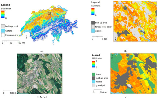
Figure 3.
LUI map for the agricultural area based on the “full model” for the whole of Switzerland (a) and two zoom levels (b,c). (c-Aerial) is an aerial orthoimage of the same area. Settlements, forest, and areas without vegetation are masked in grey, and water bodies are masked in blue.
The variation partitioning analysis showed that topo-climatic variables explain the largest part of the LUI index (individual contribution to deviance explained: 0.26, significance of contribution estimated by ANOVA: p < 0.0001), with their individual contributions greatly exceeding remote-sensing variables (individual contribution to deviance explained: 0.02, significance of contribution estimated by ANOVA: p < 0.0001; Figure 4). Despite a significant contribution by the economic output variables (ANOVA: p < 0.0001), they add the least amount of explanation (individual contribution to deviance explained: 0.01; Figure 4). For all inputs and outputs individually, topo-climatic variables explain the most deviance, while remote sensing explains large parts of pesticide and ploughing inputs. For all inputs and outputs individually, economic output variables also do not add much explanatory power.
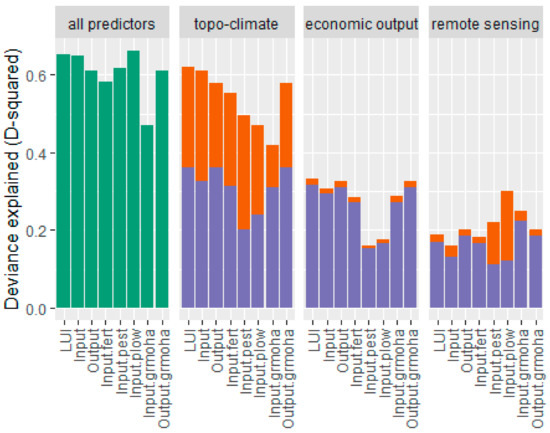
Figure 4.
Deviance explained by the full model (green), the individual contribution (orange) and the joint contribution (violet) of the topo-climatic predictors, the economic output predictors, and the remote-sensing predictors, where LUI = LUI index; Input = the input dimension of the LUI; Output = the output dimension of the LUI; Input fert = fertiliser input; Input.pest = pesticide input; Input.plow = ploughing; Input.grmoha = grazing, mowing, and harvesting; and Output.grmoha = biomass output by grazing, mowing, and harvesting.
Spatial predictions based only on one predictor set showed that topo-climatic variables defined large- to medium-scale patterns of LUI. The highest LUI was in a medium climate on terrain without slope, ridges, or depressions. Economic outputs determined medium-scale patterns with the highest LUI from grazing cattle. Remote sensing revealed local-scale patterns with highest LUI with a high mean and variation in NDVI (Figure 5).
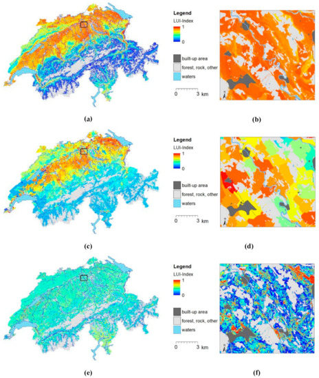
Figure 5.
LUI map based only on (a,b) climate, topography, soil, (c,d) economy, and (e,f) remote-sensing data for Switzerland (a,c,e) and the excerpt from zoom level b from Figure 3 (b,d,f).
4. Discussion
The failure to address LUI differences between and within land-cover classes has limited the scientists’ ability to make credible estimations of future responses of biodiversity to changes in land use and land cover in interaction with climate change [17,18,32]. Our results demonstrate the feasibility of using a combination of topo-climatic, economic, and remote-sensing data to map LUI at a fine scale between and within land-cover classes across the agricultural area of Switzerland. Large- to medium-scale patterns of LUI are best explained by biophysical properties (topo-climatic variables), while economic properties (economic output variables) contribute to medium-scale patterns, and the actual local agricultural management (agricultural input and biomass output, constrained by the biophysical and economic properties; remote-sensing variables), defines local patterns. To ensure a correct interpretation of our results, we discuss these points critically below.
4.1. LUI Index Parametrisation and Evaluation
LUI can be defined by inputs, outputs, and system properties [33]. Here, we addressed these LUI components for each habitat type and condensed them into one LUI index because they are not fully independent of each other [74]. The resulting index enabled the differentiation of LUI within and between land-cover classes, which is needed to better understand changes from interactions of land use, land cover, and climate change [17,18,32]. However, estimates of LUI components (fertiliser input, pesticide input, ploughing, and biomass output) were based on expert ratings rather than quantitative numbers. Moreover, in the LUI index presented here, the components are weighted equally, although their actual contributions may differ. Thus, a better conceptual understanding would be desirable for an improved LUI index. Such an understanding could be fostered by time-series analyses based on remote-sensing data, where fertiliser input, pesticide input, ploughing, grazing, mowing, harvesting, and biomass output could be monitored over the entire season (for fertilisation input, grazing, and mowing see [36]), and then be condensed into a LUI index. Nevertheless, the evaluation of the parametrised LUI index showed that it was strongly positively correlated with aerial nitrogen deposition (which represents ammonia emissions due to mineral fertiliser inputs and aspects of livestock breeding, such as grazing and manure application), the plant cover weighted mean mowing tolerance index, and the plant cover weighted mean soil nutrient content index. This indicates that the LUI index is a suitable representation of LUI.
4.2. Spatial Predictions of LUI
Since land-use activities take place in production systems that are defined by their biophysical and socio-economic properties [75], spatially explicit biophysical and socio-economic data could help to map LUI. We showed that it is feasible to map LUI using topo-climatic data, agricultural outputs, and remote-sensing data. Topo-climatic variables determine large to medium-scale patterns; the highest LUI was on medium climate terrain without slope, ridges, or depressions. Economic outputs determined medium-scale patterns with the highest LUI from grazing cattle. Remote sensing revealed local-scale patterns with the highest LUI at a high annual primary production (high average NDVI) and a high number of treatments (high variation in NDVI) [60,62].
4.3. Importance of Biophysical Factors for LUI
The variation partitioning analysis showed that topo-climatic variables explain most of the deviation of the LUI index, with their individual contributions greatly exceeding the remote-sensing data and economic output. Thus, the potential LUI predicted by biophysical factors is consistent with actual farming practices. This dominating effect of climate is in line with Holzkämper et al. [76], who showed that climate is a major driver of agricultural production. Similarly, Gerstner et al. [7] found that plant diversity was not additionally affected, and they found that in addition to land-use, environmental, and socio-economic factors had no effect on plant diversity, possibly because LUI itself is already strongly shaped by environmental and economic factors.
4.4. Suitability of Remote-Sensing Data for LUI Mapping
Remote-sensing data is already being used for mapping habitats [77], species [78], and biodiversity [25,62,79,80], and is arguably one of the most important technologies available for mapping patterns of current LUI in agricultural systems across broad geographic extents [16,35,36,37,38,42]. Nevertheless, current remote-sensing approaches have several shortcomings, and consequently our understanding of the global patterns of LUI is still weak [16]. On the one hand, existing maps have a limited extent, are too coarse, are based on model outputs instead of observations, or represent only snapshots in time that cannot describe highly dynamic land management systems [16,81]. Furthermore, current remote-sensing approaches are mostly focused on individual agricultural land-use classes (e.g., field crops [40], grassland [36]) or individual LUI components (e.g., biomass removal [42], grassland mowing frequency [39]). This may be because LUI is a complex and multidimensional phenomenon that needs a strong conceptual framework for its definition [33]. On the other hand, remote-sensing data has not been used in combination with other variables to explain these patterns [82,83]. Neglecting topo-climatic and economic output variables may not affect the results for landscapes without large environmental or economic gradients but may strongly bias predictions for more diverse landscapes. Our results show that maps produced only with remote-sensing data had a lower model quality and poorly represented medium- to large-scale patterns compared to maps that also included topo-climatic and economic output data. With our approach, which integrates a methodological framework of LUI, data from remote sensors, and ancillary data, LUI patterns can be well mapped at fine scales across large extents.
5. Conclusions
Our LUI index is a suitable representation for LUI, which can be predicted well spatially using topo-climatic, economic output, and remote-sensing predictors. Our methodology can be easily applied to other countries where habitat-type data are available – due to the worldwide availability of remote-sensing and topo-climatic data, these data should hardly represent a shortage. Given the low explanatory power of economic output variables, they may be omitted if not available.
Large- to medium-scale patterns of LUI are explained by topo-climatic predictors, while economic output predictors contribute to explaining medium-scale patterns, and remote-sensing predictors contribute to explaining local-scale patterns. The dominating effect of topo-climatic variables suggests that biophysical factors largely determine farming practices and therefore LUI, or that individual LUI components, in combination with land cover, land use, and climate descriptors, help with conducting detailed analyses of the responses of different organisms and ecosystem functions to changes in these factors. Then, with the knowledge of strong climatic influences on LUI, we may be able to make more credible estimations of the future response of different organisms, biodiversity, and ecosystem functions to land-use and land-cover changes to LUI in interaction with climate change [17,32].
With the gradual fine-scaled LUI map, it is now possible to estimate within unvarying land-use classes the effect on agrobiodiversity by an increase in LUI on fertile and accessible lands and a decrease of LUI by the abandonment of marginal agricultural lands. Further, by including thresholds, landscape configuration metrics, that are needed for instance to estimate edge effects [84] may also be derived from our finely graduated LUI maps. When deriving species-specific metrics from LUI maps, thresholds for natural areas and agricultural land use could be varied to gain a better understanding of the effects of land-use configuration on ecosystem functions.
Author Contributions
Conceptualisation, E.S.M., and A.P.; methodology, E.S.M., A.P., and A.I.; formal analysis, E.S.M., and A.P.; visualisation, E.S.M., and A.I.; writing—original draft preparation, E.S.M., A.P., A.I., and C.G.; writing—review and editing, E.S.M., A.P., and A.I. All authors have read and agreed to the published version of the manuscript.
Acknowledgments
This research was conducted as part of the ALL-EMA project, funded by the Federal Office for the Environment and the Federal Office for Agriculture.
Conflicts of Interest
The authors declare no conflict of interest. The funders had no role in the design of the study; in the collection, analyses, or interpretation of data; in the writing of the manuscript; or in the decision to publish the results.
Appendix A
Table A1.
Ratings of the land-use intensity factors and the combined LUI index per habitat type. Habitat type headings are underlined.
Table A1.
Ratings of the land-use intensity factors and the combined LUI index per habitat type. Habitat type headings are underlined.
| Habitat Type Code | Habitat Type Name | Fertiliser (Input) | Pesticide (Input) | Ploughing (Input) | Grazing, Mowing, Harvest (Input) | Grazing, Mowing, Harvest (Output) | LUI Index |
|---|---|---|---|---|---|---|---|
| 1 | Non-marine waters | ||||||
| 13 | Springs | ||||||
| 13X | Springs | 0 | 0 | 0 | 0 | 0 | 0 |
| 2 | Vegetation of banks and wetlands | ||||||
| 20 | Artificial banks | ||||||
| 20X | Artificial banks | 0 | 0 | 0 | 0 | 0 | 0 |
| 21 | Water fringe vegetation | ||||||
| 21X | Peatmoss-bladderwort bog pools, Northern perennial amphibious communities, Small reed beds of fast-flowing waters (221, 223, 224) | 0 | 0 | 0 | 0.2 | 1.6 | 0.017 |
| 212 | Reed beds | 0 | 0 | 0 | 0.4 | 3.2 | 0.033 |
| 22 | Fens and transition mires | ||||||
| 221 | Large sedge communities | 0 | 0 | 0 | 0.2 | 0.2 | 0.010 |
| 222 | Acidic fens | 0 | 0 | 0 | 0.5 | 1 | 0.028 |
| 223 | Rich fens | 0 | 0 | 0 | 0.5 | 1 | 0.028 |
| 224 | Transition mires | 0 | 0 | 0 | 0 | 0 | 0.000 |
| 225 | Arcto-alpine riverine swards | 0 | 0 | 0 | 0.2 | 0 | 0.009 |
| 23 | Humid grasslands | ||||||
| 231 | Purple moorgrass meadows and related communities | 0 | 0 | 0 | 0.8 | 8 | 0.073 |
| 232 | Atlantic and Sub-Atlantic humid meadows | 0.5 | 0.1 | 0 | 1.5 | 5 | 0.120 |
| 233 | Meadowsweet stands and related communities | 0.5 | 0 | 0 | 1 | 5 | 0.092 |
| 24 | Raised bogs | ||||||
| 241 | Bog hummocks, ridges, and lawns | 0 | 0 | 0 | 0 | 0 | 0.000 |
| 25 | Temporarily flooded annual vegetation | ||||||
| 25X | Temporarily flooded annual vegetation | 0.1 | 0 | 0 | 0.5 | 0 | 0.028 |
| 3 | Glaciers, rocks, screes, and gravel | ||||||
| 31 | Eternal snow and ice | ||||||
| 314 | Spring snow packs | 0 | 0 | 0 | 0 | 0 | 0 |
| 32 | Alluvial deposits and moraines | ||||||
| 32X | Alluvial deposits and moraines | 0 | 0 | 0 | 0 | 0 | 0.000 |
| 33 | Screes | ||||||
| 33X | Screes | 0 | 0 | 0 | 0 | 0 | 0 |
| 34 | Inland cliffs and exposed rocks | ||||||
| 34X | Inland cliffs and exposed rocks | 0 | 0 | 0 | 0 | 0 | 0 |
| 4 | Grasslands | ||||||
| 40 | Artificial grasslands and lawns | ||||||
| 401 | Temporarily grasslands in rotated crops | 5 | 0.5 | 0.3 | 5 | 110 | 1.000 |
| 403 | Lowland sowings after earthwork (road slopes...) | 0.2 | 0.1 | 0 | 1 | 30 | 0.197 |
| 404 | High altitude sowings after earthwork (ski slopes...) | 0.2 | 0.1 | 0 | 1 | 20 | 0.151 |
| 41 | Rocky flagstones and limestone pavements | ||||||
| 411 | Middle European rock debris swards | 0 | 0 | 0 | 0.1 | 0 | 0.005 |
| 412 | Stepped and garland grasslands | 0 | 0 | 0 | 0 | 0 | 0.000 |
| 413 | Middle European rock debris swards/Pavements | 0 | 0 | 0 | 0.1 | 0 | 0.005 |
| 414 | Alpine weathered rock and outcrop communities/Pavements | 0 | 0 | 0 | 0 | 0 | 0.000 |
| 42 | Thermophilus dry grasslands | ||||||
| 421 | Sub-Continental steppic grasslands | 0 | 0 | 0 | 0.8 | 2 | 0.048 |
| 422 | Sub-Atlantic very dry calcareous grasslands | 0.1 | 0 | 0 | 0.8 | 3 | 0.056 |
| 423 | Insubrian Mesobromion grasslands | 0 | 0 | 0 | 1 | 5 | 0.069 |
| 424 | Sub-Atlantic semi-dry calcareous grasslands | 0.1 | 0.1 | 0 | 2 | 15 | 0.170 |
| 43 | Unfertilised mountain grasslands and pastures | ||||||
| 431 | Blue moorgrass-evergreen sedge slopes | 0 | 0 | 0 | 0.5 | 4 | 0.041 |
| 432 | Cushion sedge carpets | 0 | 0 | 0 | 0.3 | 0 | 0.015 |
| 433 | Northern rusty sedge grasslands | 0 | 0 | 0 | 0.5 | 4 | 0.041 |
| 434 | Wind edge naked-rush swards | 0 | 0 | 0 | 0.2 | 0 | 0.009 |
| 435 | Mat-grass swards and related communities | 0.1 | 0 | 0 | 1 | 8 | 0.087 |
| 436 | Subalpine thermophile siliceous grasslands | 0 | 0 | 0 | 0 | 0 | 0.000 |
| 437 | Crooked-sedge swards and related communities | 0 | 0 | 0 | 0.5 | 1 | 0.025 |
| 44 | Snow-patches | ||||||
| 44X | Snow-patches | 0 | 0 | 0 | 0.1 | 0 | 0.005 |
| 45 | Fertilised grasslands | ||||||
| 451_LD | Medio-European lowland hay meadows (low diversity) | 4 | 0.5 | 0 | 4 | 100 | 0.848 |
| 451_MD | Medio-European lowland hay meadows (medium diversity) | 2 | 0.1 | 0 | 2.5 | 80 | 0.577 |
| 451_HD | Medio-European lowland hay meadows (high diversity) | 0.5 | 0.1 | 0 | 2 | 70 | 0.439 |
| 452_LD | Mountain and subalpine hay meadows (low diversity) | 2 | 0.1 | 0 | 2.7 | 60 | 0.495 |
| 452_MD | Mountain and subalpine hay meadows (medium diversity) | 1.5 | 0.1 | 0 | 1.8 | 35 | 0.316 |
| 452_HD | Mountain and subalpine hay meadows (high diversity) | 1 | 0.1 | 0 | 1.2 | 25 | 0.220 |
| 453_LD | Mesophilic pastures (low diversity) | 3 | 0.2 | 0 | 4 | 100 | 0.788 |
| 453_MD | Mesophilic pastures (medium diversity) | 2 | 0.5 | 0 | 2.5 | 85 | 0.618 |
| 453_HD | Mesophilic pastures (high diversity) | 0.5 | 0.1 | 0 | 1.5 | 50 | 0.324 |
| 454_LD | Rough hawkbit pastures (low diversity) | 0.5 | 0.1 | 0 | 2 | 75 | 0.461 |
| 454_MD | Rough hawkbit pastures (medium diversity) | 0.2 | 0 | 0 | 1 | 35 | 0.215 |
| 454_HD | Rough hawkbit pastures (high diversity) | 0.1 | 0 | 0 | 1 | 25 | 0.165 |
| 46 | Abandoned grasslands | ||||||
| 461 | Abandoned grasslands with Agropyron repens | 0 | 0.2 | 0 | 0.2 | 1 | 0.023 |
| 46X | Abandoned grasslands with Brachypodium pinnatum, Arrhenatherum elatius, Molinia arundinacea, or Calamagrostis varia | 0 | 0.2 | 0 | 0.5 | 2 | 0.041 |
| 5 | Woodland edges, tall herbs communities, scrubs | ||||||
| 51 | Fringes | ||||||
| 511 | Xero-thermophile fringes | 0.2 | 0.1 | 0 | 0.5 | 1 | 0.039 |
| 512 | Mesophilic fringes | 0.2 | 0.1 | 0 | 0.5 | 2 | 0.044 |
| 513 | Mixed riverine screens | 0.1 | 0.1 | 0 | 0.2 | 1 | 0.021 |
| 514 | Butterbur riverine communities | 0 | 0 | 0 | 0.1 | 0 | 0.006 |
| 515 | Shady woodland edge fringes | 0.1 | 0.1 | 0 | 1 | 3 | 0.069 |
| 52 | Clearings | ||||||
| 52X | Burdock and deadly nightshade clearings, Willowherb and foxglove clearings (521, 522) | 0 | 0 | 0 | 0.2 | 0 | 0.010 |
| 523 | Subalpine small reed meadows | 0 | 0 | 0 | 0.2 | 1 | 0.014 |
| 524 | Hercynio-alpine tall herb communities | 0 | 0 | 0 | 0.2 | 0 | 0.011 |
| 525 | Bracken fields | 0.1 | 0.1 | 0 | 0.2 | 2 | 0.026 |
| 53 | Scrubs, brushes, and clearings | ||||||
| 530 | Artificial hedgerows | 0.1 | 0.1 | 0 | 0 | 0 | 0.009 |
| 531 | Medio-European Cytisus scoparius fields | 0 | 0 | 0 | 0.5 | 2 | 0.032 |
| 532 | Blackthorn-privet scrub and box thickets | 0 | 0 | 0 | 0.5 | 1 | 0.028 |
| 533 | Blackthorn-bramble scrub | 0 | 0 | 0 | 0.1 | 0 | 0.006 |
| 534 | Bramble scrubs | 0.1 | 0.1 | 0 | 0.1 | 0 | 0.015 |
| 535 | Shrubby clearings | 0 | 0 | 0 | 0 | 0 | 0.000 |
| 536 | Pre-Alpine Willow brush | 0 | 0 | 0 | 0.5 | 0 | 0.023 |
| 537 | Mire Willow scrub | 0 | 0 | 0 | 0 | 0 | 0.000 |
| 538 | Willow brush | 0 | 0 | 0 | 0.1 | 0 | 0.005 |
| 539 | Alpine green alder scrub | 0 | 0 | 0 | 0.1 | 0 | 0.005 |
| 54 | Dry heaths | ||||||
| 541 | Sub-Atlantic acidophilous heaths | 0 | 0 | 0 | 0.5 | 1 | 0.025 |
| 542 | Juniperus sabina scrub | 0 | 0 | 0 | 0.2 | 0 | 0.010 |
| 543 | Bearberry and hairy alpenrose heaths | 0 | 0 | 0 | 0 | 0 | 0.000 |
| 544 | Juniperus nana scrub | 0 | 0 | 0 | 0.5 | 1 | 0.025 |
| 545 | Alpenrose heaths | 0 | 0 | 0 | 0.5 | 1 | 0.025 |
| 546 | Dwarf Azalea and Vaccinium heaths | 0 | 0 | 0 | 0.1 | 0 | 0.005 |
| 6 | Forests | ||||||
| 6X | Forests | ||||||
| 6XX | Forests | 0 | 0 | 0 | 0.5 | 1 | 0.028 |
| 7 | Pioneer vegetation of disturbed areas (ruderal vegetation) | ||||||
| 71 | Trampled and ruderal areas | ||||||
| 710 | Trampled ground and unvegetated ruins or debris | 1 | 0.1 | 0.1 | 0 | 0 | 0.056 |
| 711 | Flood swards and related communities | 1 | 0.1 | 0.1 | 3 | 2 | 0.204 |
| 712 | Lowland fallow fields | 1 | 0.1 | 0.1 | 3 | 2 | 0.204 |
| 713 | Subalpine and Alpine fallow fields | 1 | 0 | 0 | 2 | 30 | 0.275 |
| 714 | Annual ruderal vegetation | 0.2 | 0.1 | 0.5 | 0 | 0 | 0.037 |
| 715 | Pluriannual thermophilus ruderal vegetation | 0.1 | 0 | 0.2 | 0.2 | 0 | 0.025 |
| 716 | Pluriannual mesophilic ruderal vegetation | 0.1 | 0.1 | 0.2 | 0 | 0 | 0.019 |
| 717 | Alpine dock communities | 1 | 0.1 | 0 | 1 | 10 | 0.143 |
| 718 | Lowland dock communities | 0.1 | 0 | 0.1 | 0.2 | 0 | 0.020 |
| 72 | Anthropogenic rocky habitats | ||||||
| 720 | Unvegetated walls or paved areas | 0 | 0.2 | 0 | 0 | 0 | 0.009 |
| 721 | Vegetated ruins or old walls | 0 | 0.1 | 0 | 0 | 0 | 0.005 |
| 722 | Vegetated paved areas | 0 | 1 | 0 | 0 | 0 | 0.046 |
| 8 | Plantations, fields, and cropland | ||||||
| 81 | Cultivated ligneous formations | ||||||
| 81X | Deciduous seedbeds, Coniferous seedbeds, Chestnut groves (without undergrowth), High stem orchard | 0.1 | 4 | 0.1 | 1.1 | 5 | 0.268 |
| 815 | Low-stem orchard | 2 | 5 | 0.2 | 1.1 | 5 | 0.407 |
| 816 | Vineyards | 2 | 5 | 0.3 | 0.6 | 2 | 0.377 |
| 817 | Small fruits | 3 | 3 | 0.5 | 0.5 | 3 | 0.335 |
| 82 | Field crops | ||||||
| 82X_LD | Field crops (low diversity) | 3 | 3 | 1.5 | 2 | 100 | 0.894 |
| 82X_MD | Field crops (medium diversity) | 2 | 2 | 1.5 | 2 | 100 | 0.802 |
| 82X_HD | Field crops (high diversity) | 1.5 | 1.5 | 1.5 | 1.5 | 100 | 0.732 |
References
- Godfray, H.C.J.; Beddington, J.R.; Crute, I.R.; Haddad, L.; Lawrence, D.; Muir, J.F.; Pretty, J.; Robinson, S.; Thomas, S.M.; Toulmin, C. Food security: The challenge of feeding 9 billion people. Science 2010, 327, 812–818. [Google Scholar] [CrossRef] [PubMed]
- Meehan, T.D.; Werling, B.P.; Landis, D.A.; Gratton, C. Agricultural landscape simplification and insecticide use in the Midwestern United States. Proc. Natl. Acad. Sci. USA 2011, 108, 11500–11505. [Google Scholar] [CrossRef]
- Pe’er, G.; Dicks, L.V.; Visconti, P.; Arlettaz, R.; Báldi, A.; Benton, T.G.; Collins, S.; Dieterich, M.; Gregory, R.D.; Hartig, F.; et al. EU agricultural reform fails on biodiversity. Science 2014, 344, 1090–1092. [Google Scholar] [CrossRef] [PubMed]
- Titeux, N.; Henle, K.; Mihoub, J.-B.; Brotons, L. Climate change distracts us from equally important threats to biodiversity. Front. Ecol. Environ. 2016, 14, 291. [Google Scholar] [CrossRef]
- Newbold, T.; Hudson, L.N.; Hill, S.L.L.; Contu, S.; Lysenko, I.; Senior, R.A.; Borger, L.; Bennett, D.J.; Choimes, A.; Collen, B.; et al. Global effects of land use on local terrestrial biodiversity. Nature 2015, 520, 45–50. [Google Scholar] [CrossRef]
- Fahrig, L. Rethinking patch size and isolation effects: The habitat amount hypothesis. J. Biogeogr. 2013, 40, 1649–1663. [Google Scholar] [CrossRef]
- Gerstner, K.; Dormann, C.F.; Stein, A.; Manceur, A.M.; Seppelt, R. Effects of land use on plant diversity—A global meta-analysis. J. Appl. Ecol. 2014, 51, 1690–1700. [Google Scholar] [CrossRef]
- Seppelt, R.; Beckmann, M.; Ceauşu, S.; Cord, A.F.; Gerstner, K.; Gurevitch, J.; Kambach, S.; Klotz, S.; Mendenhall, C.; Phillips, H.R.P.; et al. Harmonizing biodiversity conservation and productivity in the context of increasing demands on landscapes. Bioscience 2016, 66, 890–896. [Google Scholar] [CrossRef]
- Foley, J.A.; Ramankutty, N.; Brauman, K.A.; Cassidy, E.S.; Gerber, J.S.; Johnston, M.; Mueller, N.D.; O’Connell, C.; Ray, D.K.; West, P.C.; et al. Solutions for a cultivated planet. Nature 2011, 478, 337–342. [Google Scholar] [CrossRef]
- MacDonald, D.; Crabtree, J.R.; Wiesinger, G.; Dax, T.; Stamou, N.; Fleury, P.; Gutierrez Lazpita, J.; Gibon, A. Agricultural abandonment in mountain areas of Europe: Environmental consequences and policy response. J. Environ. Manag. 2000, 59, 47–69. [Google Scholar] [CrossRef]
- Stoate, C.; Boatman, N.D.; Borralho, R.J.; Carvalho, C.R.; De Snoo, G.R.; Eden, P. Ecological impacts of arable intensification in Europe. J. Environ. Manag. 2001, 63, 337–365. [Google Scholar] [CrossRef] [PubMed]
- Benton, T.G.; Vickery, J.A.; Wilson, J.D. Farmland biodiversity: Is habitat heterogeneity the key? Trends Ecol. Evol. 2003, 18, 182–188. [Google Scholar] [CrossRef]
- Pereira, H.M.; Navarro, L.M.; Martins, I.S. Global Biodiversity Change: The Bad, the Good, and the Unknown. Annu. Rev. Environ. Resour. 2012, 37, 25–50. [Google Scholar] [CrossRef]
- Tasser, E.; Walde, J.; Tappeiner, U.; Teutsch, A.; Noggler, W. Land-use changes and natural reforestation in the Eastern Central Alps. Agric. Ecosyst. Environ. 2007, 118, 115–129. [Google Scholar] [CrossRef]
- Kolecka, N.; Kozak, J.; Kaim, D.; Dobosz, M.; Ginzler, C.; Psomas, A. Mapping secondary forest succession on abandoned agricultural land with LiDAR point clouds and terrestrial photography. Remote Sens. 2015, 7, 8300–8322. [Google Scholar] [CrossRef]
- Kuemmerle, T.; Erb, K.; Meyfroidt, P.; Müller, D.; Verburg, P.H.; Estel, S.; Haberl, H.; Hostert, P.; Jepsen, M.R.; Kastner, T.; et al. Challenges and opportunities in mapping land use intensity globally. Curr. Opin. Environ. Sustain. 2013, 5, 484–493. [Google Scholar] [CrossRef]
- De Chazal, J.; Rounsevell, M.D.A. Land-use and climate change within assessments of biodiversity change: A review. Glob. Environ. Chang. 2009, 19, 306–315. [Google Scholar] [CrossRef]
- Stürck, J.; Levers, C.; Van der Zanden, E.H.; Schulp, C.J.E.; Verkerk, P.J.; Kuemmerle, T.; Helming, J.; Lotze-Campen, H.; Tabeau, A.; Popp, A.; et al. Simulating and delineating future land change trajectories across Europe. Reg. Environ. Chang. 2018, 18, 733–749. [Google Scholar] [CrossRef]
- Moser, D.; Dullinger, S.; Mang, T.; Hülber, K.; Essl, F.; Frank, T.; Hulme, P.E.; Grabherr, G.; Pascher, K. Changes in plant life-form, pollination syndrome and breeding system at a regional scale promoted by land use intensity. Divers. Distrib. 2015, 21, 1319–1328. [Google Scholar] [CrossRef]
- Rüdisser, J.; Tasser, E.; Tappeiner, U. Distance to nature—A new biodiversity relevant environmental indicator set at the landscape level. Ecol. Indic. 2012, 15, 208–216. [Google Scholar] [CrossRef]
- Rüdisser, J.; Walde, J.; Tasser, E.; Frühauf, J.; Teufelbauer, N.; Tappeiner, U. Biodiversity in cultural landscapes: Influence of land use intensity on bird assemblages. Landsc. Ecol. 2015, 30, 1851–1863. [Google Scholar] [CrossRef]
- Kovács-Hostyánszki, A.; Földesi, R.; Mózes, E.; Szirák, Á.; Fischer, J.; Hanspach, J.; Báldi, A. Conservation of pollinators in traditional agricultural landscapes—New challenges in Transylvania (Romania) posed by EU accession and recommendations for future research. PLoS ONE 2016, 11, e0151650. [Google Scholar] [CrossRef] [PubMed]
- Herzog, F.; Steiner, B.; Bailey, D.; Baudry, J.; Billeter, R.; Bukácek, R.; De Blust, G.; De Cock, R.; Dirksen, J.; Dormann, C.F.; et al. Assessing the intensity of temperate European agriculture at the landscape scale. Eur. J. Agron. 2006, 24, 165–181. [Google Scholar] [CrossRef]
- Tuck, S.L.; Winqvist, C.; Mota, F.; Ahnström, J.; Turnbull, L.A.; Bengtsson, J. Land-use intensity and the effects of organic farming on biodiversity: A hierarchical meta-analysis. J. Appl. Ecol. 2014, 51, 746–755. [Google Scholar] [CrossRef]
- Rhodes, C.J.; Henrys, P.; Siriwardena, G.M.; Whittingham, M.J.; Norton, L.R. The relative value of field survey and remote sensing for biodiversity assessment. Methods Ecol. Evol. 2015, 6, 772–781. [Google Scholar] [CrossRef]
- Pereira, H.M.; Daily, G.C. Modeling biodiversity dynamics in countryside landscapes. Ecology 2006, 87, 1877–1885. [Google Scholar] [CrossRef]
- Koh, L.P.; Ghazoul, J. A matrix-calibrated species-area model for predicting biodiversity losses due to land-use change. Conserv. Biol. 2010, 24, 994–1001. [Google Scholar] [CrossRef]
- Prugh, L.R.; Hodges, K.E.; Sinclair, A.R.E.; Brashares, J.S. Effect of habitat area and isolation on fragmented animal populations. Proc. Natl. Acad. Sci. USA 2008, 105, 20770–20775. [Google Scholar] [CrossRef]
- Revilla, E.; Wiegand, T.; Palomares, F.; Ferreras, P.; Delibes, M. Effects of matrix heterogeneity on animal dispersal: From individual behavior to metapopulation-level parameters. Am. Nat. 2004, 164, E130–E153. [Google Scholar] [CrossRef]
- Bender, D.J.; Fahrig, L. Matrix structure obscures the relationship between interpatch movement and patch size and isolation. Ecology 2005, 86, 1023–1033. [Google Scholar] [CrossRef]
- Tubelis, D.P.; Lindenmayer, D.B.; Cowling, A. Bird populations in native forest patches in south-eastern Australia: The roles of patch width, matrix type (age) and matrix use. Landsc. Ecol. 2007, 22, 1045–1058. [Google Scholar] [CrossRef]
- Harfoot, M.B.J.J.; Newbold, T.; Tittensor, D.P.; Emmott, S.; Hutton, J.; Lyutsarev, V.; Smith, M.J.; Scharlemann, J.P.W.W.; Purves, D.W. Emergent global patterns of ecosystem structure and function from a mechanistic general ecosystem model. PLoS Biol. 2014, 12, 1–24. [Google Scholar] [CrossRef] [PubMed]
- Erb, K.-H.; Haberl, H.; Jepsen, M.R.; Kuemmerle, T.; Lindner, M.; Müller, D.; Verburg, P.H.; Reenberg, A. A conceptual framework for analysing and measuring land-use intensity. Curr. Opin. Environ. Sustain. 2013, 5, 464–470. [Google Scholar] [CrossRef]
- Busch, V.; Klaus, V.H.; Schäfer, D.; Prati, D.; Boch, S.; Müller, J.; Chisté, M.; Mody, K.; Blüthgen, N.; Fischer, M.; et al. Will I stay or will I go? Plant species-specific response and tolerance to high land-use intensity in temperate grassland ecosystems. J. Veg. Sci. 2019, 30, 674–686. [Google Scholar] [CrossRef]
- Estel, S.; Kuemmerle, T.; Levers, C.; Baumann, M.; Hostert, P. Mapping cropland-use intensity across Europe using MODIS NDVI time series. Environ. Res. Lett. 2016, 11, 024015. [Google Scholar] [CrossRef]
- Gómez Giménez, M.; De Jong, R.; Della Peruta, R.; Keller, A.; Schaepman, M.E. Determination of grassland use intensity based on multi-temporal remote sensing data and ecological indicators. Remote Sens. Environ. 2017, 198, 126–139. [Google Scholar] [CrossRef]
- Estel, S.; Kuemmerle, T.; Alcántara, C.; Levers, C.; Prishchepov, A.; Hostert, P. Mapping farmland abandonment and recultivation across Europe using MODIS NDVI time series. Remote Sens. Environ. 2015, 163, 312–325. [Google Scholar] [CrossRef]
- Griffiths, P.; Nendel, C.; Pickert, J.; Hostert, P. Towards national-scale characterization of grassland use intensity from integrated Sentinel-2 and Landsat time series. Remote Sens. Environ. 2020, 238, 111124. [Google Scholar] [CrossRef]
- Kolecka, N.; Ginzler, C.; Pazur, R.; Price, B.; Verburg, P.H. Regional scale mapping of grassland mowing frequency with Sentinel-2 time series. Remote Sens. 2018, 10, 1221. [Google Scholar] [CrossRef]
- Veloso, A.; Mermoz, S.; Bouvet, A.; Le Toan, T.; Planells, M.; Dejoux, J.F.; Ceschia, E. Understanding the temporal behavior of crops using Sentinel-1 and Sentinel-2-like data for agricultural applications. Remote Sens. Environ. 2017, 199, 415–426. [Google Scholar] [CrossRef]
- Denize, J.; Hubert-Moy, L.; Betbeder, J.; Corgne, S.; Baudry, J.; Pottier, E. Evaluation of using sentinel-1 and -2 time-series to identify winter land use in agricultural landscapes. Remote Sens. 2019, 11, 37. [Google Scholar] [CrossRef]
- Howison, R.A.; Piersma, T.; Kentie, R.; Hooijmeijer, J.C.E.W.; Olff, H. Quantifying landscape-level land-use intensity patterns through radar-based remote sensing. J. Appl. Ecol. 2018, 55, 1276–1287. [Google Scholar] [CrossRef]
- Verburg, P.H.; Overmars, K.P. Combining top-down and bottom-up dynamics in land use modeling: Exploring the future of abandoned farmlands in Europe with the Dyna-CLUE model. Landsc. Ecol. 2009, 24, 1167. [Google Scholar] [CrossRef]
- Allan, E.; Manning, P.; Alt, F.; Binkenstein, J.; Blaser, S.; Blüthgen, N.; Böhm, S.; Grassein, F.; Hölzel, N.; Klaus, V.H.; et al. Land use intensification alters ecosystem multifunctionality via loss of biodiversity and changes to functional composition. Ecol. Lett. 2015, 18, 834–843. [Google Scholar] [CrossRef]
- Allan, E.; Bossdorf, O.; Dormann, C.F.; Prati, D.; Gossner, M.M.; Tscharntke, T.; Bluthgen, N.; Bellach, M.; Birkhofer, K.; Boch, S.; et al. Interannual variation in land-use intensity enhances grassland multidiversity. Proc. Natl. Acad. Sci. USA 2014, 111, 308–313. [Google Scholar] [CrossRef]
- Bernhardt-Römermann, M.; Römermann, C.; Sperlich, S.; Schmidt, W. Explaining grassland biomass—The contribution of climate, species and functional diversity depends on fertilization and mowing frequency. J. Appl. Ecol. 2011, 48, 1088–1097. [Google Scholar] [CrossRef]
- Landolt, E.; Bäumler, B.; Erhardt, A.; Hegg, O.; Klötzli, F.; Lämmler, W.; Nobis, M.; Rudmann-Maurer, K.; Schweingruber, F.H.; Theurillat, J.P. Flora Indicativa—Ökologische Zeigerwerte und Biologische Kennzeichen zur Flora der Schweiz und der Alpen; Haupt: Bern, Switzerland, 2010. [Google Scholar]
- Braun-Blanquet, J. Pflanzensoziologie, Grundzüge der Vegetationskunde; Springer: Wien, Austria, 1964. [Google Scholar]
- Naimi, B.; Araújo, M.B. Sdm: A reproducible and extensible R platform for species distribution modelling. Ecography 2016, 39, 368–375. [Google Scholar] [CrossRef]
- Neter, J.; Wasserman, W.; Kutner, M. Applied Linear Regression Models; Irwin, Inc.: Homewood, IL, USA, 1983. [Google Scholar]
- Chatterjee, S.; Hadi, A.S. Regression Analysis by Example; John Wiley & Sons: Hoboken, NJ, USA, 2006. [Google Scholar]
- R Core Team. R: A language and environment for statistical computing. R Foundation for Statistical Computing, Vienna, Austria. Available online: https://www.R-project.org/ (accessed on 1 July 2019).
- ESRI. ArcGIS Desctop: Release 10.7.1; Environmental Systems Research Institute: Redlands, CA, USA, 2019. [Google Scholar]
- Swisstopo. DHM25—Das Digitale Hoehenmodell der Schweiz [DHM25—Digital Terrain Model of Switzerland]. 2005. Available online: https://shop.swisstopo.admin.ch/en/products/height_models/dhm25 (accessed on 30 January 2019).
- Hijmans, R.J.; Cameron, S.E.; Parra, J.L.; Jones, P.G.; Jarvis, A. Very high resolution interpolated climate surfaces for global land areas. Int. J. Climatol. 2005, 25, 1965–1978. [Google Scholar] [CrossRef]
- Zimmermann, N.E.; Kienast, F. Predictive mapping of alpine grasslands in Switzerland: Species versus community approach. J. Veg. Sci. 1999, 10, 469–482. [Google Scholar] [CrossRef]
- Guisan, A.; Zimmermann, N.E.N.E.; Elith, J.; Graham, C.H.; Phillips, S.; Peterson, A.T. What matters for predicting the occurrences of trees: Techniques, data, or species’ characteristics? Ecol. Monogr. 2007, 77, 615–630. [Google Scholar] [CrossRef]
- BFS and BLW. BEK200: Bodeneignungskarte der Schweiz 1:200′000 [BEK200: Soil suitability map of Switzerland]. 2000. Available online: https://www.blw.admin.ch/blw/de/home/politik/datenmanagement/geografisches-informationssystem-gis/download-geodaten.html (accessed on 30 January 2019).
- BLW. Agrarpolitisches Informationssystem AGIS. Available online: https://www.blw.admin.ch/blw/de/home/politik/datenmanagement/agate/agis.html (accessed on 30 January 2019).
- Alcaraz-Segura, D.; Lomba, A.; Sousa-Silva, R.; Nieto-Lugilde, D.; Alves, P.; Georges, D.; Vicente, J.R.; Honrado, J.P. Potential of satellite-derived ecosystem functional attributes to anticipate species range shifts. Int. J. Appl. Earth Obs. Geoinf. 2017, 57, 86–92. [Google Scholar] [CrossRef]
- Pettorelli, N.; Vik, J.O.; Mysterud, A.; Gaillard, J.M.; Tucker, C.J.; Stenseth, N.C. Using the satellite-derived NDVI to assess ecological responses to environmental change. Trends Ecol. Evol. 2005, 20, 503–510. [Google Scholar] [CrossRef] [PubMed]
- Pettorelli, N.; Wegmann, M.; Skidmore, A.; Mücher, S.; Dawson, T.P.; Fernandez, M.; Lucas, R.; Schaepman, M.E.; Wang, T.; O’Connor, B.; et al. Framing the concept of satellite remote sensing essential biodiversity variables: Challenges and future directions. Remote Sens. Ecol. Conserv. 2016, 2, 122–131. [Google Scholar] [CrossRef]
- Rihm, B.; Achermann, B. Critical loads of nitrogen and their exceedances. Swiss contribution to the effects-oriented work under the convention on long-range transboundary air pollution (UNECE). FOEN Environ. Stud. 2016, 1642, 78. [Google Scholar]
- Thornton, P.E.; Running, S.W.; White, M.A. Generating surfaces of daily meteorological variables over large regions of complex terrain. J. Hydrol. 1997, 190, 214–251. [Google Scholar] [CrossRef]
- Delarze, R.; Gonseth, Y. Lebensräume der Schweiz: Ökologie, Gefährdung, Kennarten; Ott Verlag: Thun, Switzerland, 2008; Volume 2. [Google Scholar]
- Blüthgen, N.; Dormann, C.F.; Prati, D.; Klaus, V.H.; Kleinebecker, T.; Hölzel, N.; Alt, F.; Boch, S.; Gockel, S.; Hemp, A.; et al. A quantitative index of land-use intensity in grasslands: Integrating mowing, grazing and fertilization. Basic Appl. Ecol. 2012, 13, 207–220. [Google Scholar] [CrossRef]
- Weisberg, S. Applied Linear Regression; Wiley: New York, NY, USA, 1980; ISBN 0-471-04419-9. [Google Scholar]
- Guisan, A.; Zimmermann, N.E. Predictive habitat distribution models in ecology. Ecol. Modell. 2000, 135, 147–186. [Google Scholar] [CrossRef]
- Zhang, D. A coefficient of determination for generalized linear models. Am. Stat. 2017, 71, 310–316. [Google Scholar] [CrossRef]
- Voltz, M.; Webster, R. A comparison of kriging, cubic splines and classification for predicting soil properties from sample information. J. Soil Sci. 1990, 41, 473–490. [Google Scholar] [CrossRef]
- Venables, W.N.; Ripley, B.D.; William, N.V. Modern Applied Statistics with S-Plus; Springer: New York, NY, USA, 2002. [Google Scholar]
- Borcard, D.; Legendre, P.; Drapeau, P. Partialling out the spatial component of ecological variation. Ecology 1992, 73, 1045–1055. [Google Scholar] [CrossRef]
- Real, R.; Barbosa, A.M.; Porras, D.; Kin, M.S.; Márquez, A.L.; Guerrero, J.C.; Palomo, L.J.; Justo, E.R.; Vargas, J.M. Relative importance of environment, human activity and spatial situation in determining the distribution of terrestrial mammal diversity in Argentina. J. Biogeogr. 2003, 30, 939–947. [Google Scholar] [CrossRef]
- Blüthgen, N.; Simons, N.K.; Jung, K.; Prati, D.; Renner, S.C.; Boch, S.; Fischer, M.; Hölzel, N.; Klaus, V.H.; Kleinebecker, T.; et al. Land use imperils plant and animal community stability through changes in asynchrony rather than diversity. Nat. Commun. 2016, 7, 1–7. [Google Scholar] [CrossRef] [PubMed]
- Verburg, P.H.; Crossman, N.; Ellis, E.C.; Heinimann, A.; Hostert, P.; Mertz, O.; Nagendra, H.; Sikor, T.; Erb, K.H.; Golubiewski, N.; et al. Land system science and sustainable development of the earth system: A global land project perspective. Anthropocene 2015, 12, 29–41. [Google Scholar] [CrossRef]
- Holzkämper, A.; Fossati, D.; Hiltbrunner, J.; Fuhrer, J. Spatial and temporal trends in agro-climatic limitations to production potentials for grain maize and winter wheat in Switzerland. Reg. Environ. Chang. 2014, 15, 109–122. [Google Scholar] [CrossRef]
- Tuanmu, M.N.; Jetz, W. A global, remote sensing-based characterization of terrestrial habitat heterogeneity for biodiversity and ecosystem modelling. Glob. Ecol. Biogeogr. 2015, 24, 1329–1339. [Google Scholar] [CrossRef]
- Skowronek, S.; Ewald, M.; Isermann, M.; Van De Kerchove, R.; Lenoir, J.; Aerts, R.; Warrie, J.; Hattab, T.; Honnay, O.; Schmidtlein, S.; et al. Mapping an invasive bryophyte species using hyperspectral remote sensing data. Biol. Invasions 2017, 19, 239–254. [Google Scholar] [CrossRef]
- Lausch, A.; Bannehr, L.; Beckmann, M.; Boehm, C.; Feilhauer, H.; Hacker, J.M.; Heurich, M.; Jung, A.; Klenke, R.; Neumann, C.; et al. Linking Earth Observation and taxonomic, structural and functional biodiversity: Local to ecosystem perspectives. Indic. Ecol. 2016, 70, 317–339. [Google Scholar] [CrossRef]
- Rocchini, D.; Luque, S.; Pettorelli, N.; Bastin, L.; Doktor, D.; Faedi, N.; Feilhauer, H.; Féret, J.B.; Foody, G.M.; Gavish, Y.; et al. Measuring β-diversity by remote sensing: A challenge for biodiversity monitoring. Methods Ecol. Evol. 2018, 9, 1787–1798. [Google Scholar] [CrossRef]
- Siebert, S.; Portmann, F.T.; Döll, P. Global patterns of cropland use intensity. Remote Sens. 2010, 2, 1625–1643. [Google Scholar] [CrossRef]
- He, K.S.; Bradley, B.A.; Cord, A.F.; Rocchini, D.; Tuanmu, M.N.; Schmidtlein, S.; Turner, W.; Wegmann, M.; Pettorelli, N. Will remote sensing shape the next generation of species distribution models? Remote Sens. Ecol. Conserv. 2015, 1, 4–18. [Google Scholar] [CrossRef]
- Zimmermann, N.E.; Edwards, T.C.; Moisen, G.G.; Frescino, T.S.; Blackard, J.A. Remote sensing-based predictors improve distribution models of rare, early successional and broadleaf tree species in Utah. J. Appl. Ecol. 2007, 44, 1057–1067. [Google Scholar] [CrossRef] [PubMed]
- Fahrig, L. Effects of habitat fragmentation on biodiversity. Annu. Rev. Ecol. Evol. Syst. 2003, 34, 487–515. [Google Scholar] [CrossRef]
© 2020 by the authors. Licensee MDPI, Basel, Switzerland. This article is an open access article distributed under the terms and conditions of the Creative Commons Attribution (CC BY) license (http://creativecommons.org/licenses/by/4.0/).