Article

Using FengYun-3C VSM Data and Multivariate Models to Estimate Land Surface Soil Moisture

1
State Key Laboratory of Severe Weather, Chinese Academy of Meteorological Sciences, Beijing 100081, China
2
Institution of Ecological and Agricultural Meteorology, Chinese Academy of Meteorological Sciences, Beijing 100081, China
3
College of Earth Science, Chengdu University of Technology, Chengdu 610059, China
4
Meteorological Observation Center, China Meteorological Administration, Beijing 100081, China
5
Faculty of Environment, University of Science, Vietnam National University, Ho Chi Minh City 700000, Vietnam
6
Shandong General Station of Agricultural Technology Extension, Jinan 250013, China
*
Author to whom correspondence should be addressed.
Remote Sens. 2020, 12(6), 1038; https://doi.org/10.3390/rs12061038
Submission received: 22 January 2020 / Revised: 19 March 2020 / Accepted: 21 March 2020 / Published: 24 March 2020

Abstract

:
Land surface soil moisture (SM) monitoring is crucial for global water cycle and agricultural dryness research. The FengYun-3C Microwave Radiation Imager (FY-3C/MWRI) collects various Earth geophysical parameters, and the FY-3C/MWRI SM product (FY-3C VSM) has been widely applied to determine regional-scale surface SM contents. The FY-3C VSM retrieval accuracy in different seasons was evaluated by calculating the root mean square error (RMSE), unbiased RMSE (ubRMSE), mean absolute error (MAE), and correlation coefficient (R) values between the retrieved and measured SM. A lower accuracy in July (RMSE = 0.164 cm3/cm3, ubRMSE = 0.130 cm3/cm3, and MAE = 0.120 cm3/cm3) than in the other months was found due to the impacts of vegetation and climate variations. To show a detailed relationship between SM and multiple factors, including vegetation coverage, location, and elevation, quantile regression (QR) models were used to calculate the correlations at different quantiles. Except for the elevation at the 0.9 quantile, the QR models of the measured SM with the FY-3C VSM, MODIS NDVI, latitude, and longitude at each quantile all passed the significance test at the 0.005 level. Thus, the MODIS NDVI, latitude, and longitude were selected for error correction during the surface SM retrieval process using FY-3C VSM. Multivariate linear regression (MLR) and multivariate back-propagation neural network (MBPNN) models with different numbers of input variables were built to improve the SM monitoring results. The MBPNN model with three inputs (MBPNN-3) achieved the highest R (0.871) and lowest RMSE (0.034 cm3/cm3), MAE (0.026 cm3/cm3), and mean relative error (MRE) (20.7%) values, which were better than those of the MLR models with one, two, or three independent variables (MLR-1, -2, -3) and those of the MBPNN models with one or two inputs (MBPNN-1, -2). Then, the MBPNN-3 model was applied to generate the regional SM in the United States from January 2019 to October 2019. The estimated SM images were more consistent with the measured SM than the FY-3C VSM. This work indicated that combining FY-3C VSM data with the MBPNN-3 model could provide precise and reliable SM monitoring results.

Graphical Abstract

1. Introduction

Soil moisture (SM) is a key component in the global water cycle, heat transfer, and energy exchange processes [1]. Traditional site-based methods for the acquisition of information on surface SM and other physical properties are time-consuming, expensive, and challenging to achieve at the national or global scale [2,3]. In recent decades, satellite remote sensing technology has greatly developed, and a variety of remotely sensed data have been extensively employed to retrieve and map soil water content changes over large scales and regular temporal intervals [4,5]. In recent years, microwave remote sensing has demonstrated the potential to effectively measure spatial and temporal SM variations over large areas due to its ability to penetrate clouds, rain and the atmosphere and its sensitivity to the dielectric constant [6,7]. Thus, microwave-based remote sensing has generally been considered the most promising approach for monitoring land surface SM [8].
There are two forms of microwave remote sensing, active and passive, depending on the operation mode and sensor type [6]. Numerous studies have indicated the direct and strong correlation between the surface SM content and signals collected by active and passive microwave sensors [9,10,11,12]. In general, passive microwave remote sensing observes the Earth’s surface at a shorter revisit interval than active microwave remote sensing. Additionally, passive sensors have a wider variety of mature algorithms for the retrieval of quantitative SM data, which makes it feasible to measure SM dynamics over large areas [3,13,14]. Currently, a large number of microwave-based satellite missions, such as the L-band passive microwave instruments aboard the Soil Moisture Active Passive (SMAP) satellite launched by the National Aeronautics and Space Administration (NASA) in 2015, the SM and Ocean Salinity (SMOS) satellite launched by the European Space Agency (ESA) in 2009, the Advanced Microwave Scanning Radiometer for Earth observation science (AMSR-E) and the Advanced Microwave Scanning Radiometer-2 (AMSR-2) onboard the EOS-Aqua satellite, and China’s Microwave Radiometer Imager (MWRI) onboard the FengYun-3 (FY-3) series satellites, have been frequently employed for global SM monitoring [8,15,16,17,18].
Although passive microwave remote sensing is an effective approach for providing regional SM estimates under all weather conditions, its monitoring accuracy is likely to be affected by land surface features, such as vegetation coverage and roughness. Many researchers have proposed solutions to correct for the effects of vegetation and roughness on surface emissivity by assimilating multisource data [19], developing a microwave-based vegetation index [7], applying an iterative algorithm [20], and enhancing the radiation transfer equation [14]. Choi and Hur [20] downscaled the AMSR-E SM products from a spatial resolution of 25 km to 1 km, and then combined the AMSR-E and Moderate-resolution Imaging Spectroradiometer (MODIS) data to monitor SM in Korea from May 1 to September 30, 2007. The disaggregated SM products achieved a better statistical error between the ground-measured and AMSR-E SM values, and the integration of AMSR-E and MODIS products appeared to be an effective method for improving microwave SM products, with the minimum root mean square error (RMSE) values decreasing from 0.131 to 0.059, and the maximum RMSE values decreasing from 0.179 to 0.171. Liu et al. [19] produced a merged SM product by combining AMSR-E and Advanced Scatterometer (ASCAT) data, and the results showed that the proposed methodology had the potential to rescale and improve the accuracy of SM retrievals. Shi et al. [14] proposed a dual-polarization inversion technique to minimize the effects of surface roughness, and the developed technique has been proven to be useful for achieving more accurate global SM estimations using the available satellite instruments. Wang et al. [7] developed a microwave vegetation water index (MVWI) by combining the vegetation water content (VWC) index and a vegetation structure parameter, making it possible to evaluate the VWC along with the SM.
A number of researchers have evaluated the relationships among multisource data to enhance SM products [21,22]. De Jeu et al. [21] researched the distribution of correlations between the SMOS and AMSR-E products using the classic linear regression model, and high correlations were found between the two products in moderately vegetated areas, while the correlations were low in densely vegetated regions. Ma and Liu [22] used a back-propagation (BP) neural network model to analyze the potential of using optical vegetation information and a combination of polarizations (HH and HV) for SM inversion. The results indicated that HV was more strongly related to SM than HH, and the addition of optical vegetation information to microwave remote sensing data for SM retrieval increased the average R value by more than 0.05.
Among these soil moisture products, the FY-3/MWRI SM (FY-3 VSM) is an official SM product released by the National Satellite Meteorological Center (NSMC) of China and has been widely used to record the soil moisture content in the top layer with a spatial resolution of 25 km [18,23]. The FY-3 VSM products are retrieved from observations via the MWRI onboard FY-3 series satellites, including FY-3A, FY-3B, FY-3C, and FY-3D. Generally, the FY-3C VSM product is considered to have a better quality than FY-3A and FY-3B, and longer available time series data than FY-3D. Zhu et al. [23] assessed the performance of FY-3C VSM over cropland in Henan Province, China, during 2016, and the results indicated that the SM variation patterns of the FY-3C VSM retrievals were in good agreement with the measured SM. However, the FY-3C VSM tended to overestimate or underestimate the SM during the year. To further improve the performance of the FY-3C VSM, various algorithms and models should be established and applied to enhance the FY-3C VSM product and achieve more accurate SM estimations.
This paper aimed to improve the accuracy of surface SM (0–5 cm) estimates by combining multisource data, including satellite data, optical vegetation information, elevation, and location data. For this purpose, the FY-3C VSM product and MODIS normalized difference vegetation index (NDVI) time series for the months from January 2019 to October 2019 were reprojected and resampled. The international soil moisture network (ISMN) measurement database was employed as the reference SM data. Then, a quantile regression (QR) model was used to analyze the detailed correlation between the surface SM and multiple factors. Multivariate models, including multivariate linear regression (MLR), and multivariate BP neural network (MBPNN), were developed to correct for the effects of vegetation coverage and enhance the monitoring of SM over large regions. Additionally, the SM images retrieved from FY-3C VSM, which were estimated by the best model and interpolated from the ISMN, were compared, and statistical parameters were calculated to further validate the feasibility of using the proposed method to enhance satellite SM products.

2. Data and Methods

2.1. Multisource Data

2.1.1. Data from the ISMN

SM measurements are a valuable resource for assuring the consistent and precise quality of various satellite-derived SM products [24]. The ISMN is an international cooperation that has provided and maintained globally available in situ SM measurements at various depths since 1952 [25]. Currently, the ISMN contains information from more than 60 networks and over 2500 stations around North America, Europe, Asia, Australia, Africa, and South America [26].
Given the widespread distribution and large number of ground-based SM observations in the U.S. (Figure 1), this region (67°03′W–124°76′W and 25°24′N–49°39′N) was selected as the study area in this paper. Most parts of the study area have continental and subtropical climates, with average temperatures in January and July ranging from −3 °C and 24 °C in the northern part to 11 °C and 28 °C in the southern part, respectively. The average annual rainfall in the area decreases from 1500 mm over the central plain and Pacific coasts to 500 mm over the western plateau, where the highest elevation is 4187 m.
Approximately 700 SM sites operated by three SM networks, i.e., the U.S. Climate Reference Network (USCRN), Snow Telemetry (SNOTEL), and Soil-Climate Analysis Network (SCAN), are located in the study area (Figure 1). The hourly data sets at 0.05-m depth from January 1 at 00:00 to October 31 at 23:00 in 2019 were collected and generated as the actual SM in this study. The sampling interval of the original data was one hour, and the time interval of the measurements was converted into one month using the averaging method.
Then, the empirical Bayes kriging (EBK) method and ArcMap software were employed for spatial interpolation and to achieve the monthly SM over the study area (Figure 2). Here, the output size of the cell was set as 0.27756061° to assure the same spatial resolution as the microwave remote sensing data. The mean prediction error and RMSE of the spatial interpolation using EBK were 0.0025 cm3/cm3 and 0.096 cm3/cm3, respectively, which indicated high accuracy between the ground-based and interpolated SM in the study area. According to Figure 2, the SM content in the midwestern part was significantly lower than that in the eastern and northwestern parts of this region, which is basically consistent with the patterns of rainfall variations and climate types.

2.1.2. FY-3C VSM

FY-3 series satellites, including FY-3A, FY-3B, FY-3C, and FY-3D, are China’s second generation of polar-orbiting meteorological satellites and are operated by the China Meteorological Administration (CMA). These satellites are equipped with various instruments in the optical, infrared, and microwave bands and have become valuable data sources for global climate predictions, weather forecasting and surface SM measurements over the past decade [27,28]. The MWRI onboard FY-3 includes vertical and horizontal polarization modes (V/H) in the 10.65-GHz, 18.7-GHz, 23.8-GHz, 36.5-GHz, and 89.0-GHz frequency bands [29]. The characteristics, such as the bandwidth, sensitivity, calibration accuracy, scanning mode, and instantaneous field of view (IFOV), are shown in Table 1 [23]. Among all of the frequency bands, the channels in the 10.65 GHz band are capable of penetrating clouds and rain and are mainly used to obtain global surface sea temperature (SST), wind speed, SM content, and other geophysical parameters under all weather conditions.
FY-3C was launched in September 2013 and has been recognized as the first official service satellite and a suitable replacement for FY-3A as the new forenoon satellite [30]. FY-3C VSM products are retrieved from the L1 brightness temperature (BT) data collected by MWRI using a new inversion technique, i.e., the Qp model, which was built using advanced integral equation (AIE) model simulations of microwave emissions [14]. Compared with the single channel SM retrieval algorithm, both the vertical and horizontal polarizations of the X-band (10.65 GHz) were applied in the Qp model to decrease the effects of roughness and vegetation coverage [23]. Also, the pixels covered with snow, frozen soil, and coastal waters were removed from the FY-3C VSM retrievals. These products are classified into ascending (A) and descending (D) products at daily, 10-day, and monthly time intervals, and have been widely used to detect the global land surface soil volumetric water content (cm3/cm3) with a spatial resolution of 25 km. In this study, the monthly FY-3C VSM products (FY3C_MWRIX_GBAL_L3_VSM.HDF) data from January to October 2019 were downloaded from the website of the NSMC (satellite.nsmc.org.cn/) and reprojected from the equal-area scalable earth (EASE) grid 2.0 to the WGS-84 grid.

2.1.3. MODIS NDVI

The NDVI products derived from MODIS are the most mature and widely used source for monitoring vegetation status and estimating soil water contents at the regional scale as supplemental data in many previous studies [20,23]. Here, 14 tiles (h08v04, h08v05, h08v06, h09v04, h09v05, h09v06, h10v04, h10v05, h10v06, h11v04, h11v05, h12v04, h12v05, and h13v04) of monthly MODIS NDVI products (MOD13A3, v006) from the Terra satellite from January 2019 to October 2019 were downloaded from the NASA website (https://ladsweb.modaps.eosdis.nasa.gov/). The MODIS NDVI products were reprojected from sinusoidal to WGS-84, and their spatial resolutions were resampled from 250 m to 25 km to be consistent with the FY-3C VSM.
Apart from the FY-3C VSM and MODIS NDVI, the elevation was derived from the GMTED2010 elevation dataset and resampled to 25 km as well. Then, the values of ISMN, FY-3C VSM, MODIS NDVI, elevation, latitude, and longitude of the study area were extracted pixel by pixel for multivariate correlation analysis and comprehensive monitoring of SM.

2.2. Multivariate Models

2.2.1. Quantile Regression Model

A key objective of this paper was to indicate the detailed relationship between SM measurements and remotely sensed surface features and other potential impact factors, such as vegetation and location information. In previous studies, regression models were extensively applied to quantitatively analyze the relationships among various factors. However, most regression models were conducted based on the correlation between dependent and independent variables at the mean level. Therefore, the information reflected by those models is limited [31]. In addition, the distribution characteristics of random errors are strictly required when ordinary least squares (OLS) method is used for regression analysis. Thus, the linear assumption of least squares may be too harsh when applying the OLS to some practical problems [32].
The quantile is the proportion of dependent variables which are lower than a certain element in the sorted array. For example, the quantile 0.1 represents for the first 10 elements in the array with 100 elements arranged from the lowest to the highest, which makes it possible for quantiles to represent any location in the distribution. QR theory was developed by Koenker and Bassett [33] as a tool for overcoming the limitations of classic OLS and comprehensively reflecting the conditional distribution characteristics under different quantiles. The QR model was built based on the conditional quantile of dependent variables, which makes it capable of describing the impacts of independent variables on the shapes and variation ranges of the conditional distributions of dependent variables. A number of researchers have applied QR in many fields, including economics, medicine, education, and social and environmental sciences, to achieve steady and robust regression results [34,35].
Compared with the OLS-based model, the QR model provides an in-depth view of the relationship between independent and dependent variables [34]. Let the distribution function of the random variable Y be F(y) = P(Yy). The quantile function of Y at the τ (0< τ <1) quantile can be defined as
Q ( τ ) = inf { y : F ( y ) τ }
The loss function, which is a piecewise function (Figure 3), is defined as
ρ τ ( z ) = z ( τ I z < 0 ( z ) ) = { τ z z 0 ( τ 1 ) z z < 0
where I(·) is the indicative function.
Let z equal y y ^ , and ρτ(z) can be represented by
ρ τ ( y y ^ ) = τ ( y y ^ ) I ( y y ^ 0 ) + ( τ 1 ) ( y y ^ ) I ( y y ^ < 0 )
Then, the τth QR of y ( y ^ ) can be estimated by minimizing the expected loss:
min y ^ R E [ τ ( y y ^ ) I ( y y ^ 0 ) + ( τ 1 ) ( y y ^ ) I ( y y ^ < 0 ) ]
Assume that the linear regression equation is described as
Y = X β + ε
where Y is the dependent variable, X’ is the transpose of independent X, β is the regression coefficient, and ε is the error term. The regression coefficient β in a conditional QR is estimated by minimizing the sum of absolute deviation [32]:
min β R [ ( i : y i x i β ( τ ) ) n τ | y i x i β ( τ ) | + ( i : y i < x i β ( τ ) ) n ( 1 τ ) | y i x i β ( τ ) | ]
Currently, the simplex algorithm, interior point algorithm, and smoothing algorithm are commonly used to estimate the regression efficiency β(τ). Among those algorithms, the smoothing algorithm is suitable for processing datasets with a large number of observations and variables and was thus applied in this study. Then, the τth (0 < τ < 1) quantile function of y can be represented by
Q y ( τ | x ) = x β ( τ )
where β(τ) is the solution to the minimizing problem in Equation (6). Thus, many regression lines at different quantiles can be obtained to examine the behavior of the response variable beyond the average of the Gaussian distribution [36].

2.2.2. Back-Propagation Neural Network Model

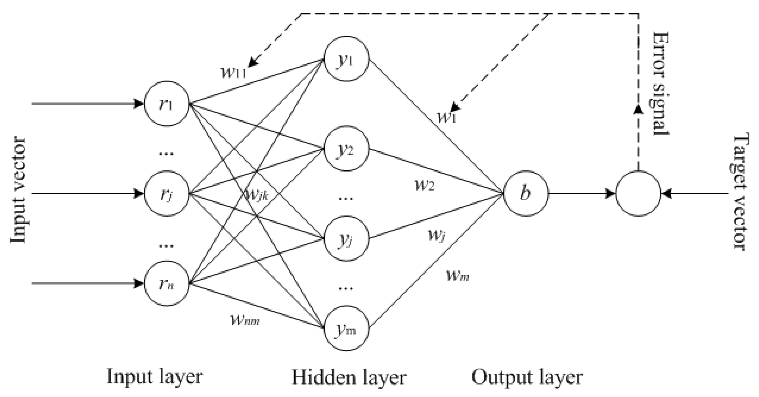
Neural networks (NNs) are flexible and intelligent computing frameworks for solving large-scale and nonlinear problems over a broad range of applications, such as time series data forecasting and soil property estimation [3,22,37,38]. The back-propagation neural network (BPNN), developed by Rumelhart et al. [39] in 1985, has been recognized as the most mature and widespread method in the field of NNs and usually demonstrates superior simulation capability [5,40]. The learning process of the BPNN consists of forward propagation of the data stream in the “input layer→hidden layers→output layer” direction and back propagation of the error signal in the “output layer→hidden layers→input layer” direction, as shown in Figure 4.
Suppose a three-layer BPNN has n inputs, m neurons in the hidden layer, and one output (Figure 4). The weights and thresholds from the input to hidden layer are wjk and θk (j = 1, 2, …, n; k = 1, 2, …, m), and the weights and thresholds from the hidden to output layer are wk (k = 1, 2, …, m) and θ, respectively. Then, the kth unit of the hidden layer (yk) and the output of the output layer (b) can be given as Equations (8) and (9), respectively.
y k = f ( j = 1 n w j k r j θ k )
b = f ( k = 1 m w k y k θ )
where f represents the sigmoid function, which is described as
f ( x ) = [ 1 + exp ( x ) ] 1
The mean square error (e) between the actual output (b) and target vector (T) is calculated as follows:
e = 1 N k = 1 N ( b k T k ) 2
where N represents the number of samples in the target vector.
The weights and thresholds are continuously adjusted to meet the error limit during the BP process of the error signal. In general, the gradient descent with momentum (GDM) method is helpful to speed up the learning process and prevent it from being trapped in poor local minima. Thus, this method has been widely applied as the training method in BPNNs [38,39]. The training efficiency and accuracy are highly relevant to the initial setting of parameters, such as the learning rate (η), iterations (t), and momentum term (α), when the GDM method is used in the training process of BPNN [5]. The regulating rules of weights and thresholds are shown in Equations (12)–(15). After the adjustment of weights and thresholds, the well-trained BPNN is used to map SM based on the inputs provided.
w k ( t 1 ) = w k ( t ) + η δ y t + α [ w k ( t ) w k ( t 1 ) ]
w j k ( t 1 ) = w j k ( t ) + η δ k y j + α [ w j k ( t ) w j k ( t 1 ) ]
θ ( t 1 ) = θ ( t ) + η δ + α [ θ ( t ) θ ( t 1 ) ]
θ k ( t 1 ) = θ k ( t ) + η δ k + α [ θ k ( t ) θ k ( t 1 ) ]
In this study, three multivariate BPNN (MBPNN) models with one, two, and three input variables were established using the MATLAB Neural Network Toolbox for estimating SM in the U.S. For this purpose, the FY-3C VSM and MODIS NDVI, together with the location information, were generated and extracted as the input variables of the MBPNN models. The measured SM from the ISMN data was set as the target vector in these models. The “newff” function was used to design a BPNN, the “sim” function was used to calculate the output of the network, and the “mse” function was applied to calculate the performance errors. Additionally, the GDM method was employed to train the samples, and the learning rate, momentum coefficient, iteration and error limit were set as 0.05, 0.95, 10,000, and 0.00001, respectively, based on the comparison experiments. Of the samples, 80% and 20% were set as the training and testing sets, respectively, and the model yielded the best training and testing accuracies to simulate the SM values of each pixel.

2.2.3. Linear Regression Model

The linear regression model has been extensively used for interpretation of the change in the dependent variable using one or more independent variables in various fields, and it can be defined as
Y = β0 + β1 × 1 + β2x2 + … + βnxn + ε
where x1, x2, …, xn are independent variables, Y is the dependent variable, β0 is a constant, βi (i = 1, 2, …, n) are coefficients of xi (i = 1, 2, …, n), and ε is the residual error.
In this study, three linear regression models (MLR-1, MLR-2, and MLR-3) with 1~3 influence factors as independent variables and ground-based SM from ISMN as the dependent variable were established for SM estimation. The types of independent variables in each MLR model and inputs in each MBPNN model are listed in Table 2.

2.3. Statistical Indicators

To evaluate the accuracies of FY-3C VSM products and the monitored SM using multivariate models, five statistical indicators, including the correlation coefficient (R), RMSE, unbiased RMSE (ubRMSE), mean absolute error (MAE), and mean relative error (MRE), were adopted in this study.
The R and MRE represent the relative accuracy between the FY-3C VSM retrievals or the estimated SM and the SM measurements, respectively. To evaluate the FY-3C VSM accuracy, R and MRE can be defined by Equations (17) and (18).
R = i 1 N ( V S M i V S M ¯ ) ( S M i S M ¯ ) i 1 N ( V S M i V S M ¯ ) 2 i 1 N ( S M i S M ¯ ) 2
MRE = 1 N i = 1 N | V S M i S M i | S M i × 100 %
where VSMi represents the FY-3C VSM retrievals (cm3/cm3), SMi represents the SM measurements (cm3/cm3), V S M   ¯ represents the average of FY-3C VSM retrievals (cm3/cm3) across all pixels in the study area, S M ¯     indicates the average of SM measurements (cm3/cm3), and N represents the total number of valid samples and varies for each month.
The RMSE, ubRMSE, and MAE evaluate the absolute difference of FY-3C VSM product or SM estimations from the measured SM via the ISMN, which can be calculated by the following equations.
RMSE = i = 1 N ( V S M i S M i ) 2 N
ubRMSE = RMSE 2 MD 2
MAE = 1 N i 1 N | V S M i S M i |
where MD is the abbreviation of the mean deviation, which can be calculated as
MD = 1 N i = 1 N ( V S M i S M i )

3. Results and Analysis

3.1. Comparison between FY-3C VSM and Measured SM

To assess the consistency between the FY-3C VSM and the measured SM in different seasons, pixel values were extracted from FY-3C VSM images and the measured SM from the ISMN in January, April, July, and October 2019. Considering the periodic change of SM curves between different rows, the pixels in one cycle were representative and should be selected to describe the over- and underestimation issues of FY-3C VSM directly. Here, 150 pixels were selected randomly from the central rows with the latitude ranging from 32.19°N to 32.74°N in each month for comparison between the FY-3C VSM product and measured SM. The variation curves of FY-3C VSM (red line) and measured SM (green line) are displayed in Figure 5. Generally, the varying patterns of the FY-3C retrievals were basically consistent with the in situ SM values in most samples during the four months, especially in January (Figure 5a), whose pixel values from both sources were distributed between 0.10 cm3/cm3 and 0.45 cm3/cm3. In February 2019 (Figure 5b), the FY-3C VSM sample values from 10 to 50 were basically lower than the SM measurements, and the sample values from 70 to 130 were mainly higher than the measured SM values. It was obvious that the FY-3C satellite retrievals in July 2019 (Figure 5c) overestimated the SM in almost of the samples, and the estimation error was significantly greater than that in the other months, which was possibly due to the potential impacts caused by factors such as deep and widespread vegetation coverage in summer. The curves for October 2019 (Figure 5d) indicated a similar situation to that in July, although the proportion and degree of overestimation were slightly decreased compared with those in July. To further evaluate the vegetation impact on the FY-3C VSM retrieval accuracy in July, the SM deviations between the FY-3C VSM and the measured SM were calculated and compared to the MODIS NDVI by plotting the variation curves and evaluating the correlation between the two sources. The plot could be found in the Appendix A, where the curves of the MODIS NDVI (red line) and the SM deviations (green line) showed a similar variation pattern and the R value was 0.666, which indicated a strong correlation between the NDVI and SM deviation.
To further analyze the SM monitoring accuracy using the FY-3C VSM product, the values of R, RMSE, ubRMSE, and MAE between the FY-3C VSM and the in situ SM measurements in different months were calculated pixel by pixel, as shown in Table 3. All valid pixels from the FY-3C VSM products in January (4464), April (8870), July (7446), and October (8852) were included in the statistical error metrics in Table 3. The values of R were distributed between 0.467 and 0.621, indicating a moderate or strong correlation between FY-3C VSM and the actual SM in all seasons. The SM estimation accuracies in January (RMSE = 0.116 cm3/cm3, ubRMSE = 0.113 cm3/cm3, and MAE = 0.092 cm3/cm3) and April (RMSE = 0.114 cm3/cm3, ubRMSE = 0.112 cm3/cm3, and MAE = 0.094 cm3/cm3) were significantly higher than those in July (RMSE = 0.164 cm3/cm3, ubRMSE = 0.130 cm3/cm3, and MAE = 0.120 cm3/cm3) and October (RMSE = 0.147 cm3/cm3, ubRMSE = 0.121 cm3/cm3, and MAE = 0.113 cm3/cm3). Among these months, despite the high correlation between the estimated and actual SM, the SM inversion in July yielded the worst accuracy due to overestimation.

3.2. Relationship between Multiple Variables and SM Measurements

By evaluating of the FY-3C VSM and multiple related factors, such as vegetation, slope, and location, against the measured SM using the QR model, we aimed to correct for bias and improve the SM inversion accuracy that was described in Section 3.1.
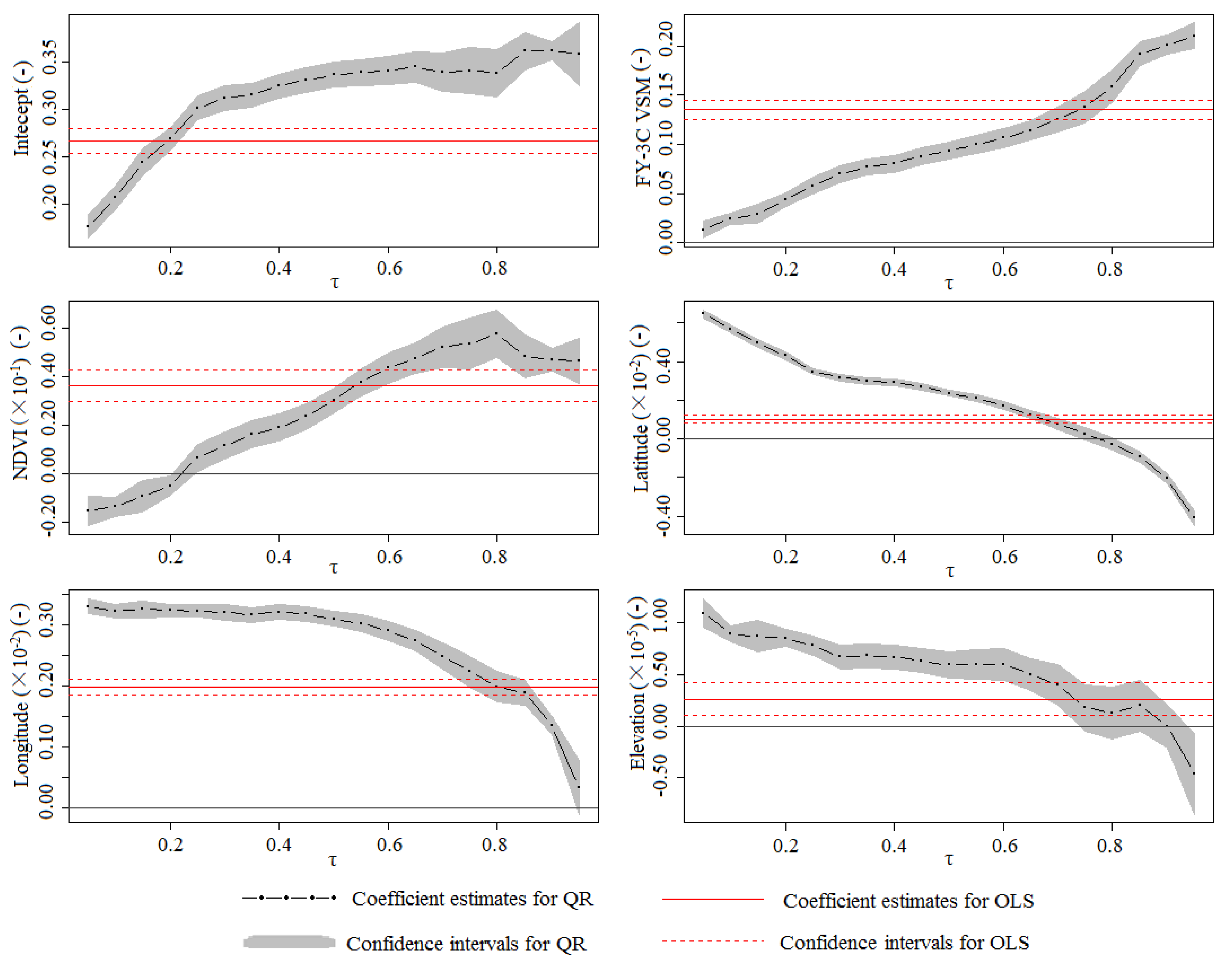
In Figure 6, the dependent variable, i.e., the measured SM, was plotted against quantiles from 0.05 to 0.95 for five independent variables, including the FY-3C VSM retrievals, MODIS NDVI, latitude, longitude, and elevation, and an intercept using the “quantreg” package in R (https://www.R-project.org/). The plots depicted the variation pattern of coefficient estimates and 95% confidence intervals of all independent variables and intercept. According to Figure 6, the FY-3C VSM had a positive correlation with the measured SM at all quantiles, and the QR coefficient estimates increased from 0.01 in the lower quantile to 0.22 in the upper quantile. The estimate from the OLS method was constant at approximately 0.14, which suggested that the estimated SM using OLS was likely to be overestimated in areas with low soil water contents (dry) and underestimated in areas with high soil water contents (wet). Apart from the FY-3C VSM, the MODIS NDVI had negative estimates at quantiles from 0 to 0.2 and positive estimates at quantiles from 0.2 to 0.95. The coefficient estimates showed an increasing trend before reaching their peak (0.06) at quantile 0.8 and then slightly decreased to 0.04. The latitude and elevation had both negative (quantiles 0.8–0.95) and positive (0.05–0.8) effects on SM, and the latitude was more significant than elevation at all quantiles. The longitude had a positive correlation with SM at all quantiles, and its coefficient estimates decreased from the lower to upper quantiles.
The QR models were created at five quantiles (0.1, 0.3, 0.5, 0.7, and 0.9), and their coefficient estimates and significant P values were calculated, as presented in Table 4. Table 4 indicates that the linear relationship between the measured SM and the abovementioned multiple independent variables varied at different quantiles. For FY-3C VSM, latitude and longitude, the p values were lower than 0.001 at all quantiles, which indicated a high and stable correlation between the SM measurements and those input variables. At the 0.1 quantile, the larger p value was found in the NDVI, which indicated a lower correlation between the NDVI and the ground-based SM measurements than between that and the other variables. The p values of elevation at quantiles 0.7 (0.001) and 0.9 (0.992) were greater than those of the other inputs, indicating a lower correlation between elevation and measured SM at high quantiles. All of the regression models passed the significance test at the 0.005 level except for the elevation at the 0.9 quantile. Thus, the FY-3C VSM, MODIS NDVI, latitude, and longitude were selected as the input variables for improving the accuracy of SM monitoring.

3.3. SM Estimation Using Multivariate Models

3.3.1. Multivariate Models for SM Estimation

The issue with SM overestimation was relatively more serious in summer (July) among all of the seasons, as demonstrated in Section 3.1. Six multivariate models (MLR-1, MLR-2, MLR-3, MBPNN-1, MBPNN-2, and MBPNN-3) were built and compared to improve the SM estimation accuracy in July. The R, RMSE, MAE, and MRE values between the actual and estimated SM using those models were calculated pixel-by-pixel and are shown in Table 5. It is obvious that the performances of the models with two (MLR-2 and MBPNN-2) or three (MLR-3 and MBPNN-3) independent or input variables were improved compared with the models with only FY-3C VSM (MLR-1 and MBPNN-1) as the independent or input variable. The MLR-1 and MLR-2 models obtained higher monitoring accuracy than the MBPNN-1 and MBPNN-2 models, which was possibly due to the disadvantages of the BPNN, such as the limited sample number, overfitting, and trivial linear case inclusion. The addition of location information significantly enhanced the accuracy of SM estimates in models MLR-3 and MBPNN-3, and the performance of MBPNN-3 (R = 0.871, RMSE = 0.034 cm3/cm3, and MAE = 0.026 cm3/cm3, MRE = 20.7%) was the best among all of the models, followed by MLR-3 (R = 0.694, RMSE = 0.047 cm3/cm3, MAE = 0.035 cm3/cm3, and MRE = 27.3%).
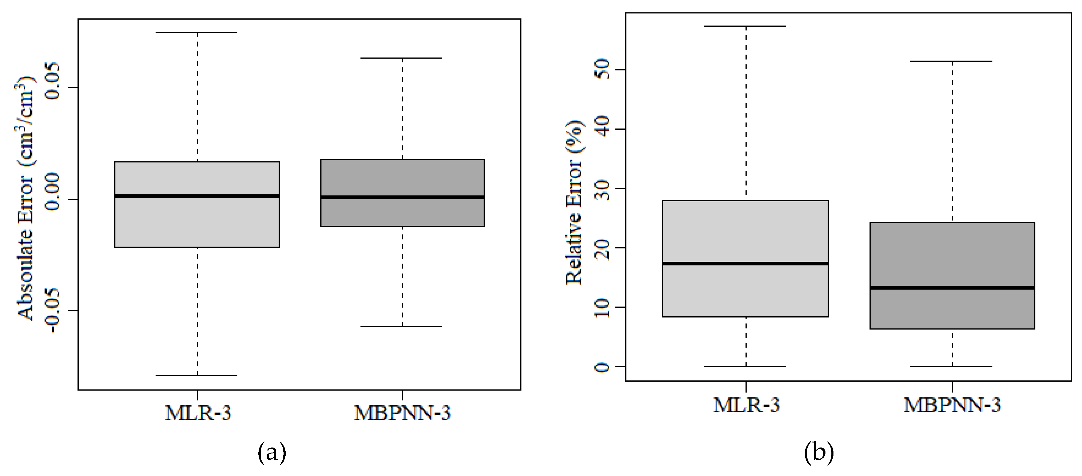
To further validate the accuracy of the SM estimations using MLR-3 and MBPNN-3, the distribution of absolute error and relative error between the actual and estimated SM in the pixels are depicted in Figure 7. Generally, MBPNN-3 demonstrated better performance than MLR-3, with lower median values of the absolute (0.00 cm3/cm3) and relative (14.0%) errors than MLR-3. Additionally, the distribution ranges of the MLR-3 errors between the 25% (Q1) and 75% (Q3) quantiles, which were [−0.02, 0.02] for absolute errors and [11.0%, 28.0%] for relative errors, were both wider and overall larger than those for the MBPNN-3, whose absolute and relative errors between Q1 and Q3 were distributed between [−0.01, 0.02] and [7.5%, 25.0%], respectively. The results indicate that the multivariate nonlinear model is a suitable and promising approach for achieving SM estimation results with high accuracy.

3.3.2. Regional SM Monitoring Results

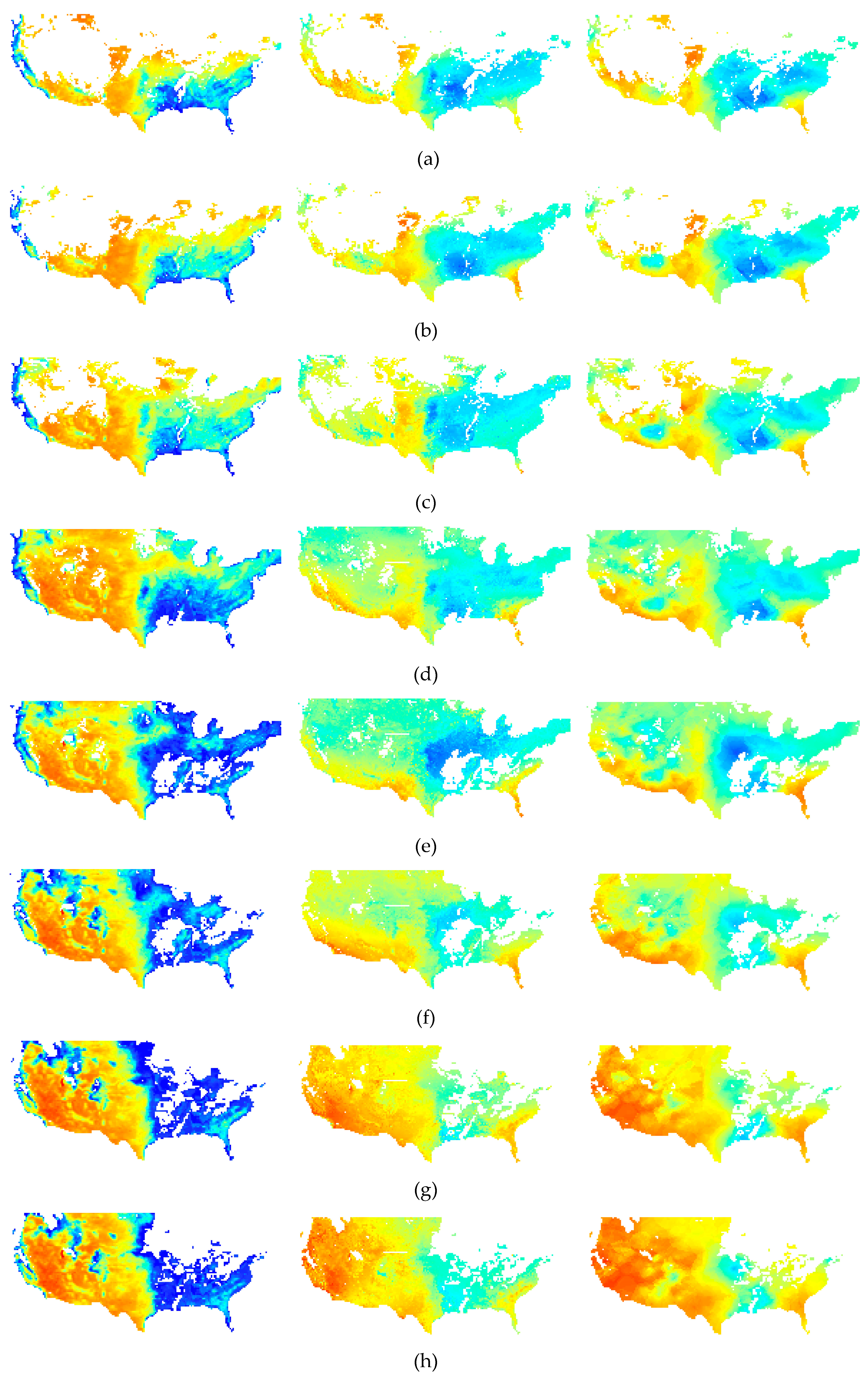
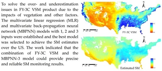
Here, the MBPNN-3 model was applied to estimate the regional SM in the study area from January to October 2019, as shown in the middle column of Figure 8. The images in the left and right columns are the FY-3C VSM retrievals and the measured SM from the ISMN. In general, the FY-3C VSM products overestimated the SM in the eastern part and underestimated the SM in the midwestern part of the U.S. during the 10 months. It was evident that the spatiotemporal variation patterns of the SM estimations using the MBPNN-3 model were more consistent with the in situ SM measurements than those using the FY-3C VSM products. The over- and underestimation issues were reduced in the estimated SM images throughout the study area, especially the overestimation problem in the western and northeastern parts, indicating that the MBPNN-3 model with the FY-3C VSM and supplementary information (vegetation and location) as inputs was applicable for providing reliable SM estimations. Dry areas with SM values lower than 0.20 cm3/cm3 were found in the southwestern part, and the proportion of dry areas gradually increased from January to July and slightly decreased from August to October. The wet areas with SM values greater than 0.30 cm3/cm3 were mainly located in the mideastern region, and the proportions of wet area during January to July were slightly greater than those from July to October.

3.3.3. Accuracy Assessment between the Estimated and Actual SM

To further validate the SM estimation accuracy, the R, RMSE, MAE, and MRE values between the estimated and actual SM, as well as the number of samples in each month from January to October 2019, were calculated, as shown in Table 6. The R values in each month were distributed between 0.787 and 0.943, and the RMSE, MAE, and MRE values in each month in 2019 were all lower than 0.063 cm3/cm3, 0.054 cm3/cm3, and 46.7%, respectively, indicating that the SM estimation accuracy in the U.S. was generally high during all months. The SM estimation accuracy varied in different months. The highest SM estimation accuracy was found in February (R = 0.943, RMSE = 0.030 cm3/cm3, MAE = 0.022 cm3/cm3, and MRE = 10.4%), followed by January (R = 0.913, RMSE = 0.040 cm3/cm3, MAE = 0.031 cm3/cm3, and MRE = 15.4%). The worst accuracy was found in September (R = 0.862, RMSE = 0.063 cm3/cm3, MAE = 0.054 cm3/cm3, and MRE = 46.7%), followed by October and August. In conclusion, the established MBPNN-3 model yielded accurate and acceptable SM estimations in all seasons and can be employed to improve the monitoring accuracy of regional surface soil moisture.

4. Discussion

The enhancement of the FY-3C VSM product using SM measurements and multivariate models improved its feasibility for land surface SM monitoring. In this study, the in situ SM measurements from ISMN played an important role during processes such as the retrieval accuracy evaluation of FY-3C VSM, the relationship analysis of various input variables, the establishment of multivariate models, and the validation of SM estimation accuracy. A large number of representative stations in the U.S. made it possible to map the SM measurements across the whole study area and adequate training and testing samples for the MLR and MBPNN models. Therefore, widespread and accurate SM measurements are crucial and indispensable data sources for enhancing satellite products. The interpolation method allows the spatial resolution consistency between the satellite and in situ SM data. However, the SM prediction accuracy needs to be further improved.
Although the established MBPNN-3 model with FY-3C VSM, MODIS NDVI, latitude, and longitude as inputs enhanced the SM retrievals from the pure satellite products, the estimation accuracy varied in different seasons due to the seasonal variations in land surface features and the impacts of other factors. The seasonal differences in the relationships between SM and vegetation coverage and in the climate distribution should be studied to further improve the accuracy of SM estimations in future research.

5. Conclusions

Assessing the consistency between the FY-3C VSM and measured SM indicated an issue with overestimation due to the impacts caused by factors such as vegetation. Thus, a comprehensive evaluation of multiple factors is necessary to improve the SM inversion accuracy from the FY-3C VSM. In this case, QR models were applied to provide a detailed depiction of the relationship between SM and multisource factors, including the FY-3C VSM, MODIS NDVI, elevation, latitude, and longitude. The results showed that the FY-3C VSM and longitude had a positive correlation with SM in all quantiles, and the MODIS NDVI, latitude, and elevation had both positive and negative effects in the different quantiles. The coefficient estimates of those factors all passed the significance test at the 0.005 level at each quantile between [0.1, 0.9], except for the elevation at quantile 0.9.
In this study, six multivariate models, including MLR-1, MLR-2, MLR-3 MBPNN-1, MBPNN-2, and MBPNN-3, were employed to estimate regional SM in July. The assessment of model performance showed that the SM estimation accuracy was improved with the increase in the number of independent or input variables for both linear and nonlinear models. The MBPNN-3 achieved the highest SM estimation accuracy and was thus used to estimate SM in the U.S. from January to October 2019. The FY-3C VSM retrievals, estimated SM using MBPNN-3 and the measured SM images, were compared, and the R values and estimation errors between the actual SM measurements and SM estimations in each month were calculated. The results showed that the spatiotemporal characteristics of the estimated SM using MBPNN-3 were more consistent with the actual SM than those estimated using the FY-3C VSM retrievals. The values of R were distributed between 0.787 and 0.943, and the RMSE, MAE, and MRE values were less than 0.063 cm3/cm3, 0.054 cm3/cm3, and 46.7%, respectively, which demonstrated the feasibility of using the MBPNN-3 model to improve the SM monitoring accuracy at the regional scale.

Author Contributions

L.W. and S.F. designed the study. L.W. implemented the experiments and conducted the data analysis. Z.P. and Y.Z. downloaded and processed the FY-3C/MWRI, MODIS NDVI and meteorological data. S.F., D.N.K. and W.H. reviewed and edited the manuscript. L.W. led, and all authors have read and agreed to the published version of the manuscript.

Funding

This research was funded by Ministry of Science and Technology of the People’s Republic of China, grant number 2018YFC1506500. The APC was funded by Chinese Academy of Meteorological Sciences, grand number 2019Z010.

Acknowledgments

This manuscript was supported by the National Key Research and Development Programs of China under Grant 2018YFC1506500 and the Fundamental Research Fund under Grant 2019Z010.

Conflicts of Interest

The authors declare no conflict of interest.

Appendix A

See Figure A1 here.
Figure A1. Variation curves of the MODIS NDVI and SM deviation between FY-3C VSM and measured SM.
Remotesensing 12 01038 g0a1

References

  1. Crow, W.T.; Kustas, W.P.; Prueger, J.H. Monitoring root-zone soil moisture through the assimolation of a thermal remote sensing-based soil moisture proxy into a water balance model. Remote Sens. Environ. 2008, 112, 1268–1281. [Google Scholar] [CrossRef]
  2. Zhang, J.; Zhang, Q.; Bao, A.; Wang, Y. A new remote sensing dryness index based on the near-infrared and red spectral space. Remote Sens. 2019, 11, 456. [Google Scholar] [CrossRef] [Green Version]
  3. Chang, D.-H.; Islam, S. Estimation of Soil Physical Properties Using Remote Sensing and Artificial Neural Network. Remote Sens. Environ. 2000, 74, 534–544. [Google Scholar] [CrossRef]
  4. Singh, V.K.; Singh, B.P.; Kisi, O.; Kushwaha, D.P. Spatial and multi-depth temporal soil temperature assessment by assimilating satellite imagery, artificial intelligence and regression based models in arid area. Comput. Electron. Agric. 2018, 150, 205–219. [Google Scholar] [CrossRef]
  5. Wang, L.; Wang, P.; Liang, S.; Qi, X.; Li, L.; Xu, L. Monitoring maize growth conditions by training a BP neural network with remotely sensed vegetation temperature condition index and leaf area index. Comput. Electron. Agric. 2019, 160, 82–90. [Google Scholar] [CrossRef]
  6. Barrett, B.W.; Dwyer, E.; Whelan, P.E. Soil Moisture Retrieval from Active Spaceborne Microwave Observations: An Evaluation of Current Techniques. Remote Sens. 2009, 1, 210–242. [Google Scholar] [CrossRef] [Green Version]
  7. Wang, L.; Li, Z.; Chen, Q.; Wei, X. A microwave vegetation water index from passive microwave radiometer data. Int. J. Remote Sens. 2008, 29, 6779–6787. [Google Scholar] [CrossRef]
  8. Sabaghya, S.; Walker, J.P.; Renzullo, L.J.; Jackson, T.J. Spatially enhanced passive microwave derived soil moisture: Capabilities and opportunities. Remote Sens. Environ. 2018, 209, 551–580. [Google Scholar] [CrossRef]
  9. O’Neill, P.E. Microwave remote sensing of soil moisture: A comparison of results from different truck and aircraft platforms. Int. J. Remote Sens. 1985, 6, 1125–1134. [Google Scholar]
  10. Lee, K.H.; Anagnostou, E.N. A combined passive/active microwave remote sensing approach for surface variable retrieval using Tropical Rainfall Measuring Mission observations. Remote Sens. Environ. 2004, 92, 112–125. [Google Scholar] [CrossRef]
  11. Huang, S.; Tsang, L.; Njoku, E.G.; Chan, K.S. Backscattering coefficients, coherent reflectivities, and emissivities of randomly rough soil surfaces at L-Band for SMAP applications based on numerical solutions of maxwell equations in three-dimensional simulations. IEEE Trans. Geosci. Remote Sens. 2010, 48, 2557–2568. [Google Scholar] [CrossRef]
  12. He, B.; Xing, M.; Bai, X. A synergistic methodology for soil moisture estimation in an alpine prairie using radar and optical satellite data. Remote Sens. 2014, 6, 10966–10985. [Google Scholar] [CrossRef] [Green Version]
  13. Njoku, E.G.; Li, L. Retrieval of land surface parameters using passive microwave measurements at 6–18 GHz. IEEE Trans. Geosci. Remote Sens. 1999, 37, 79–93. [Google Scholar] [CrossRef] [Green Version]
  14. Shi, J.; Jiang, L.; Zhang, L.; Chen, K.-S.; Wigneron, J.-P.; Chanzy, A.; Jackson, T.J. Physically based estimation of bare-surface soil moisture with the passive radiometers. IEEE Trans. Geosci. Remote Sens. 2006, 44, 3145–3153. [Google Scholar] [CrossRef]
  15. Entekhabi, D.; Nakamura, H.; Njoku, E.G. Solving the inverse problem for soil moisture and temperature profiles by sequential assimilation of multifrequency remotely sensed observations. IEEE Trans. Geosci. Remote Sens. 1994, 32, 438–447. [Google Scholar] [CrossRef]
  16. Lievens, H.; Tomer, S.K.; Bitar, A.A.; De Lannoy, G.J.M.; Drusch, M.; Dumedah, G.; Hendricks Franssen, H.-J.; Kerr, Y.H.; Martens, B.; Pan, M.; et al. SMOS soil moisture assimilation for improved hydrologic simulation in the Murray Darling Basin, Australia. Remote Sens. Environ. 2015, 168, 146–162. [Google Scholar] [CrossRef]
  17. Njoku, E.G.; Chan, S.K. Vegetation and surface roughness effects on AMSR-E land observations. Remote Sens. Environ. 2006, 100, 190–199. [Google Scholar] [CrossRef]
  18. Cui, C.; Xu, J.; Zeng, J.; Chen, K.-S.; Bai, X.; Lu, H.; Chen, Q.; Zhao, T. Soil moisture mapping from satellites: An intercomparison of SMAP, SMOS, FY3B, AMSR2, and ESA CCI over two dense network regions at different spatial scales. Remote Sens. 2018, 10, 33. [Google Scholar] [CrossRef] [Green Version]
  19. Liu, Y.Y.; Parinussa, R.M.; Dorigo, W.A.; de Jeu, R.A.M.; Wagner, W.; van Dijk, A.I.J.M.; McCabe, M.F.; Evans, J.P. Developing an improved soil moisture dataset by blending passive and active microwave satellite-based retrievals. Hydrol. Earth Syst. Sci. 2011, 15, 425–436. [Google Scholar] [CrossRef] [Green Version]
  20. Choi, M.; Hur, Y. A microwave-optical/infrared disaggregation for improving spatial representation of soil moisture using AMSR-E and MODIS products. Remote Sens. Environ. 2012, 124, 259–269. [Google Scholar] [CrossRef]
  21. De Jeu, R.A.M.; Wagner, W.; Holmes, T.R.H.; Dolman, A.J.; van de Giesen, N.C.; Friesen, J. Global Soil Moisture Patterns Observed by Space Borne Microwave Radiometers and Scatterometers. Surv. Geophys. 2008, 29, 399–420. [Google Scholar] [CrossRef] [Green Version]
  22. Ma, H.; Liu, S. The potential evaluation of multisource remote sensing data for extracting soil moisture based on the method of BP neural network. Can. J. Remote Sens. 2016, 42, 117–124. [Google Scholar] [CrossRef]
  23. Zhu, Y.; Li, X.; Pearso, S.; Wu, D.; Sun, R.; Johnson, S.; Wheeler, J.; Fang, S. Evaluation of Fengyun-3C soil moisture products using in-Situ data from the Chinese Automatic Soil Moisture Observation Stations: A case study in Henan Province, China. Water 2019, 11, 248. [Google Scholar] [CrossRef] [Green Version]
  24. Dorigo, W.A.; Wagner, W.; Hohensinn, R.; Hahn, S.; Paulik, C.; Xaver, A.; Gruber, A.; Drusch, M.; Mecklenburg, S.; van Oevelen, P.; et al. The International Soil Moisture Network: A data hosting facility for global in situ soil moisture measurements. Hydrol. Earth Syst. Sci. 2011, 15, 1675–1698. [Google Scholar] [CrossRef] [Green Version]
  25. Dorigo, W.A.; Gruber, A.; de Jeu, R.A.M.; Wagner, W.; Stacke, T.; Loew, A.; Albergel, C.; Brocca, L.; Chung, D.; Parinussa, R.M.; et al. Evaluation of the ESA CCI soil moisture product using ground-based observations. Remote Sens. Environ. 2015, 162, 380–395. [Google Scholar] [CrossRef]
  26. The Data Hosting Facility of the International Soil Moisture Network. Available online: https://ismn.geo.tuwien.ac.at/en/ (accessed on 10 December 2019).
  27. Wang, L.; Hu, X.; Chen, L.; He, L. Consistent calibration of VIRR reflective solar channels onboard FY-3A, FY-3B, and FY-3C using a multisite calibration method. Remote Sens. 2018, 10, 1336. [Google Scholar] [CrossRef] [Green Version]
  28. Wang, D.; Liang, S.; He, T.; Cao, Y.; Jiang, B. Surface shortwave net radiation estimation from FengYun-3 MERSI data. Remote Sens. 2015, 7, 6224–6239. [Google Scholar] [CrossRef] [Green Version]
  29. Zhao, X.; Chen, N.; Li, W.; Peng, J.; Shen, L. ℓp-ICP coastline inflection method for geolocation error estimation in FY-3 MWRI data. Remote Sens. 2019, 11, 1886. [Google Scholar] [CrossRef] [Green Version]
  30. Zhang, Y.; Kan, X.; Ren, W.; Cao, T.; Tian, W.; Wang, J. Snow cover monitoring in Qinghai-Tibetan plateau based on Chinese Fengyun-3/VIRR data. J. Indian Soc. Remote Sens. 2017, 45, 271–283. [Google Scholar] [CrossRef]
  31. Fournier, J.M.; Koske, I. Public employment and earnings inequality: An analysis based on conditional and unconditional quantile regressions. Econ. Lett. 2013, 121, 263–266. [Google Scholar] [CrossRef]
  32. Koenker, R.; Hallock, K.F. Quantile regression. J. Econ. Perspect. 2001, 15, 143–156. [Google Scholar] [CrossRef]
  33. Koenker, R.; Bassett, G.J. Regression quantiles. J. Electrochem. Soc. 1987, 46, 33–50. [Google Scholar]
  34. Arunraj, N.S.; Ahrens, D. A hybrid seasonal autoregressive integrated moving average and quantile regression for daily food sales forecasting. Int. J. Prod. Econ. 2015, 170, 321–335. [Google Scholar] [CrossRef]
  35. Rocchini, D.; Cade, B.S. Quantile regression applied to spectral distance decay. IEEE Geosci. Remote Sens. 2008, 5, 643. [Google Scholar] [CrossRef]
  36. Benoit, D.F.; Van den Poel, D. Benefits of quantile regression for the analysis of customer lifetime value in a contractual setting: An application in financial services. Expert Syst. Appl. 2009, 36, 10475–10484. [Google Scholar] [CrossRef]
  37. Babu, C.N.; Reddy, B.E. A moving-average filter based hybrid ARIMA–ANN model forforecasting time series data. Appl. Soft Comput. 2014, 23, 27–38. [Google Scholar] [CrossRef]
  38. Khashei, M.; Bijari, M.; Hejazi, S.R. Combining seasonal ARIMA models with computational intelligence techniques for time series forecasting. Soft Comput. 2012, 16, 1091–1105. [Google Scholar] [CrossRef]
  39. Rumelhart, D.E.; Hinton, G.E.; Williams, R.J. Learning representations by back-propagating errors. Nature 1986, 326, 533–536. [Google Scholar] [CrossRef]
  40. Zhang, Y.; Wu, L. Stock market prediction of S&P 500 via combination of improved BCO approach and BP neural network. Expert Syst. Appl. 2009, 36, 8849–8854. [Google Scholar]
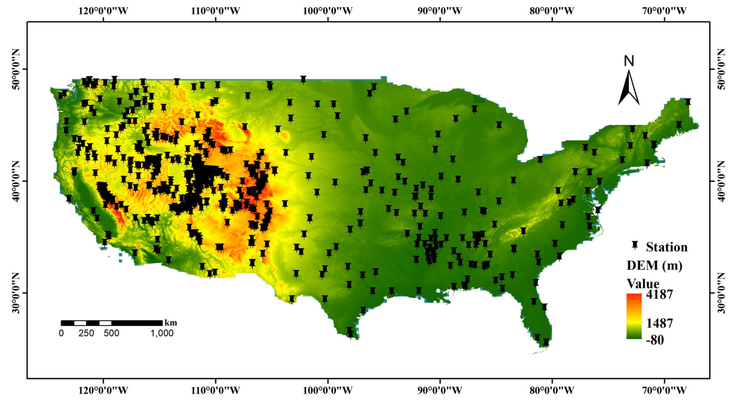
Figure 1. The location of the study area and the distribution of SM stations.
Remotesensing 12 01038 g001
Figure 2. Interpolated ISMN values in January 2019 using the empirical Bayes kriging (EBK) method.
Remotesensing 12 01038 g002
Figure 3. Loss function (ρτ(z)) of the quantile regression (QR).
Remotesensing 12 01038 g003
Figure 4. Basic structure of a three-layer back-propagation neural network (BPNN).
Remotesensing 12 01038 g004
Figure 5. Comparison between the FY-3C VSM and measured soil moisture (SM) in different seasons. (a)–(d) show the comparison curves for January, April, July, and October 2019, respectively.
Remotesensing 12 01038 g005aRemotesensing 12 01038 g005b
Figure 6. Coefficients of intercept and multiple variables under different quantiles.
Remotesensing 12 01038 g006
Figure 7. (a) Absolute errors and (b) relative errors between the measured and estimated SM using MLR-3 and MBPNN-3 models.
Remotesensing 12 01038 g007
Figure 8. FY-3C VSM retrievals, estimated SM using MBPNN-3 and measured SM in the U.S. from January to October 2019. (a)–(j) are the SM monitoring results in January, February, March, April, May, June, July, August, September, and October 2019, respectively.
Remotesensing 12 01038 g008aRemotesensing 12 01038 g008b
Table 1. Characteristics of FY-3 Microwave Radiation Imager (MWRI) channels.
Frequency (GHz)10.6518.723.836.589
PolarizationV/HV/HV/HV/HV/H
Band width (MHz)1802004009004600
Sensitivity (K)0.50.50.80.51.0
Calibration accuracy (K)1.51.51.51.51.5
IFOV (km × km)51 × 8530 × 5027 × 4518 × 309 × 15
Pixel size (km × km)40 × 11.240 × 11.220 × 11.220 × 11.210 × 11.2
Dynamic range (K)3~340
Sampling number240
Beam efficiency≥90%
Beam error (°)<0.1
Scanning modeConical scanning
Orbit width (km)1400
Viewing angle (°)45 ± 0.1
Scanning period (s)1.7 ± 0.1
Scanning period error (ms)0.34 ms (between scanning lines)/1 ms (in 30 min)
Table 2. Independent/input variables of the multivariate linear regression (MLR) and multivariate back-propagation neural network (MBPNN) models.
ModelIndependent/Input Variable
MLR-1, MBPNN-1FY-3C VSM
MLR-2, MBPNN-2FY-3C VSM, MODIS NDVI
MLR-3, MBPNN-3FY-3C VSM, MODIS NDVI, location
Table 3. Root mean square error (RMSE), unbiased RMSE (ubRMSE), mean average error (MAE), and correlation coefficient (R) values between the measured SM and FY-3C VSM retrievals in different months.
Error MetricsRRMSE (cm3/cm3)ubRMSE (cm3/cm3)MAE (cm3/cm3)
Month
January0.4670.1160.1130.092
April0.5000.1140.1120.094
July0.6210.1640.1300.120
October0.5580.1470.1210.113
Table 4. Coefficients and significance tests for the QR.
τ0.10.30.50.70.9
Variable β(τ)Pβ(τ)Pβ(τ)Pβ(τ)Pβ(τ)P
Intercept0.207<0.0010.311<0.0010.336<0.0010.339<0.0010.361<0.001
FY-3C VSM0.024<0.0010.070<0.0010.094<0.0010.125<0.0010.201<0.001
NDVI
(×10−1)
−0.136=0.0050.116<0.0010.304<0.0010.523<0.0010.470<0.001
Latitude
(×10−2)
0.568<0.0010.318<0.0010.235<0.0010.077<0.001−0.207<0.001
Longitude
(×10−2)
0.323<0.0010.321<0.0010.310<0.0010.248<0.0010.135<0.001
Elevation
(×10−5)
0.891<0.0010.667<0.0010.591<0.0010.399=0.001−0.001=0.992
Table 5. Correlation coefficient and error metrics between the estimated and actual SM values using the MLR and MBPNN models.
Error MetricsRRMSE (cm3/cm3)MAE (cm3/cm3)MRE (%)
Model
MLR-10.6400.0500.03932.0
MBPNN-10.6900.0560.04438.0
MLR-20.6610.0490.03830.4
MBPNN-20.7080.0540.04135.2
MLR-30.6940.0470.03527.3
MBPNN-30.8710.0340.02620.7
Table 6. Correlation coefficient and error metrics between the estimated and actual SM values from January to October 2019 using the MBPNN-3 model.
Error MetricsRRMSE
(cm3/cm3)
MAE (cm3/cm3)MRE
(%)
Number of Samples
Month
January0.9130.0400.03115.44464
February0.9430.0300.02210.45501
March0.7870.0560.04321.76690
April0.8930.0320.02411.08870
May0.8240.0470.03918.18391
June0.8630.0350.02715.17701
July0.8710.0340.02620.77446
August0.8700.0520.04236.37366
September0.8620.0630.05446.78001
October0.8440.0530.04344.38852