Abstract
Cultural ecosystem services (CES) are a significant part of the ecosystem and are considered to be a core component of human welfare and ecosystem protection. CES have been historically difficult to quantitatively evaluate because of their subjectivity and intangibility. Additionally, their evolution over time has rarely been explored. Here, we quantitatively evaluated various CES and generated corresponding value index (VI) maps. We then further explored the evolution of CES characteristics over space and time. We selected Xi’an as the study area and applied the Social Values of Ecosystem Services (SolVES) model to evaluate CES and generate three specific VI maps. A system dynamics model based on socioeconomic and survey data of CES for each administrative division was established. Finally, we simulated four developmental scenarios in order to predict potential developmental changes of CES in 2030 under these different scenarios. This study provides a method for evaluating CES and explores the application of system dynamics to different fields. Additionally, our findings may provide guidance for the formulation of regional policies and support missions to improve civilizations within ecological systems, coordinate future economic growth with ecosystem services, and achieve sustainable development.
1. Introduction
Ecosystem services (ES) are the various benefits that human beings derive from ecosystems and can be seen as the contribution of natural capital to human well-being, including the supply of both tangible material products and the provision of intangible services [1,2,3,4]. The Millennium Ecosystem Assessment identifies four types of ES: provisioning, regulating, cultural, and supporting services. Cultural ecosystem services (CES) are a significant part of the human ecosystem and are defined as non-material benefits derived from the ecosystem through spiritual enrichment, cognitive improvement, ideological inspiration, entertainment, and aesthetic experience [5]. Additionally, CES are also considered a core component of human welfare and ecosystem protection [6]. Therefore, it is beneficial to evaluate CES and improve our understanding of the interaction between our ecosystem and society, as well as their impact on our potential happiness [7].
Scholars have recently begun to try to evaluate CES from the perspective of society and space [8]. Maria Johansson took a bottom-up approach to assess CES in peri-urban wetland areas [9]. Jared Retka used social media data to characterize CES for a large marine protected area (MPA) in northeast Brazil and outline management opportunities and implications [10]. Participatory approaches are helpful in assessing the social complexity of CES and are particularly useful in data-poor regions. Rémi Jaligot applied a Participatory Geographic Information System (PGIS) to assess the evolution of CES in peripheral areas in developing countries [11]. Geo-tagged photo data shared on social media networks makes it possible to assess CES and landscape features, and to inform urban planning [12,13,14,15]. Coupling current approaches for recreation management at country level with behavioral data derived from surveys and population distribution data. A method is proposed to map and evaluate outdoor recreation service. Considering that all ecosystems are potential providers of services, this is measured by the extent and quality of citizens’ access to nature [16,17]. There are indications that the type and level of stakeholder participation is important for the evaluation of CES [18]. It is significant to consider that CES should evolve over both space and time. CES research should consider not only the current CES but also predict the need for future CES in order to provide decision makers with needed information [19,20]. At present, the dynamic evolution of CES and the prediction under different scenarios need imperative further research.
System dynamic (SD) models are based on control theory, systems theory, and information theory and are used to study the structure, function, and development of a feedback system [21]. The main feature of the SD model is the ability to simulate complex systems dynamically, so as to examine the development and behavioral trends of complex systems under different scenarios (different parameters or different policy factors) and provide support to decision makers with different needs [22,23,24]. SD modelling has been applied to ecology, landscape ecology, and urban development research, and has become a new developmental trend [25,26,27]. Sarai Pouso modelled recreational fishing activity using a SD model in order to analyze the effects that future management decisions and unexpected environmental changes [28]. A modelling framework combined SD models with land-use change models to simulate landscape ecosystem service value (ESV), used to explore the potential impact of land-use changes on ESV [29]. The resource management of the Jiading Wetland was examined by applying group model building and SD [30]. The spatial and temporal differences of the forest ecological security early warning index values from 2009 to 2015 were analyzed using the SD model, and the evolution trend of forest ecological security was predicted from 2015 to 2030 [31]. An ecological-economic model was developed by integrating conventional economic input-output (IO) within SD [32]. Additionally, results showed that SD enabled for predictive forecasting at multiple geographic levels making use of spatially explicit information and landscape metrics. Yet there is still a gap in the simulations applied to CES [33]. Rita Lopes and Nuno Videira presented a structured methodology to conduct a collaborative process of deepening understanding of ES with a Participatory Systems Mapping (PSM) approach. Through stakeholders’ engagement it was possible to develop a collaborative construction of causal loop diagrams depicting understand feedback loops in ES simulations [34]. An assessment of provisioning services in Scotland from 1940–2016 using integrated accounting methods shows that fundamental changes in farming systems will occur over time. Relationships between landscape functions and ES changing over time [35]. The Multiscale Integrated Model of Ecosystem Services model is an SD framework that can be used to simulate future ES including CES by coupling human and natural systems [36]. Through the above scholars’ research on the application of SD model to ES, we choose SD model to realize the dynamic change simulation of CES.
Xi’an was known as Chang’an in the past and is the capital of Shaanxi Province. It was the starting point of the Silk Road, the core area of the Belt and Road construction, and an important central city in western China [37]. Xi’an has been voted one of China’s best tourist destinations and one of the best cities in China’s international image, with six heritage sites on the World Heritage List [38]. In 2017, Xi’an received 18,931,400 domestic and foreign tourists, with total tourism revenue of 163.330 billion RMB. In February 2018, the National Development and Reform Commission, the Ministry of Housing and Urban-Rural Development of the People’s Republic of China issued the “Guangzhong Plain Urban Agglomeration Development Planning” to support Xi’an in building a national central city, an international comprehensive transportation hub, and building an international metropolis with historical and cultural characteristics. CES of Xi’an play a profound role in both historical status and future construction, therefore, Xi’an is chosen as our research area.
In this study, we quantitatively and spatially evaluated the regional CES in 13 districts of Xi’an city and studied the dynamic changes of CES under different scenarios. We established a database of natural environmental data and social survey data, using the SolVES model to analyze the distribution and characteristics of CES factors. We then used SD software to establish a dynamic model of the CES of each administrative division of Xi’an city. We simulated different developmental scenarios in order to explore predicted impacts of different CES in 2030. Four scenarios were set up to simulate the future development of Xi’an. The results provide insights into future developmental models for each district of Xi’an city, and also help guide the sustainable development decision-making in government planning.
2. Materials and Methods
2.1. Study Area
Xi’an is located between 107.40°~109.49°E and 33.42°~34.45°N, which is in the central part of the Guanzhong Plain of China, as shown in Figure 1. The southern part of Xi’an is backed by the Qinling Mountains. This city has the Weihe River, the Jinghe River, the Heihe River, the Bahe River, and other rivers with abundant water resources and fine vegetation development conditions. It has 13 districts (Xincheng, Beilin, Lianhu, Yanta, Baqiao, Weiyang, Yanliang, Lintong, Chang’an, Gaoling, Huyi, Lantian, Zhouzhi), with a total area of 10752 km2. The profound history and culture provide a unique cultural foundation for Xi’an’s CES.
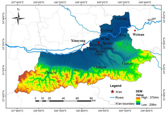
Figure 1.
The location map of study area.
2.2. Available Data
We used 2017 social and economic data (annual statistics) from the Xi’an Bureau of Statistics. Social survey data were from a questionnaire survey of 13 districts. A total of 960 random sampling survey questionnaires were distributed to respondents in the study area, resulting in 839 valid cases and 87.4% questionnaire efficiency. Table 1 shows the characteristics of the sample.

Table 1.
Respondent’s characteristics.
The content of the questionnaire was divided into four parts. Part one included information about the social background of the respondents. Part two included information that affected the validity of the questionnaire, including whether the respondent was familiar with the area and whether any types of CES were obtained. Part three included attitude and preference information. Part four included VI information, which involved the respondents scoring the CES in this area. After an on-the-spot investigation of the natural and cultural environment of Xi’an, we selected three CES in this region for evaluation that included recreation, historical, aesthetic values. Table 2 illustrates the classification and connotation of the three CES. We have correspondingly localized the descriptions in the table for better expression.
Table 2.
The descriptions of cultural ecosystem services (CES) types.
In the process of modelling and quantifying CES, in addition to social survey data, the designated geographic database also requires multiple environmental index data representing the characteristics of the natural environment within the study area. The basic environmental index data were derived from Landsat 8 cloudless images and GDEMDEM 30-m resolution digital elevation model data (ELEV) from the Computer Network Information Center. Land use and land cover (LULC) data was obtained by interpreting remote sensing images using ENVI 5.1 through supervised classification. SLOPE and HILLSHADE Digital elevation model data was extracted using ArcGIS10.2 surface analysis tools. Distance from road (DTR) and water (DTW) was determined using a horizontal distance layer extracted from ArcGIS10.2 distance mapping tool and based on road networks and the nearest water feature (lake, pond, rivers, creek, spring point, etc.). The spatial resolution of each environmental index grid layer was 30 m.
The administrative boundaries of each district were obtained from the national basic information center. Basic vector data, such as roads and rivers, came from the Arceyes software. Detailed data sources are shown in Table 3.
Table 3.
Data sources.
2.3. Methodology
2.3.1. Quantification of CES
The SolVES model is a GIS application developed by the USGS Geosciences and Environmental Change Science Center (GECSC) and it can comprehensively evaluate, quantify, and map CES such as aesthetics, education, recreation, culture, and heritage. SolVES combines both natural and human factors for a comprehensive assessment that not only accounts for natural environmental impacts, but constraints from human factors as well. SolVES uses social-values mapping research to implement a methodology for integrating social values into the CES assessment process by quantifying and mapping these values through “ Value Index” (VI) (0–10), which provides a spatial, nonmonetary metric statistically related to the environmental characteristics of the study area itself. The greater VI, the higher value of the CES. The Maxent maximum entropy modelling software (Maxent) embedded in SolVES can explain the relationship between CES and environmental variables, which enables a complete visual mapping of the evaluation results [39,40,41].
Geospatial and social survey data are used in SolVES as inputs into three submodules: the ecosystem services social-values model, the value mapping model, and the value transfer mapping model. Each submodule has its own specific function and can simultaneously be associated with the other submodules and script data to perform additional calculations. In this study, we used SolVES (version 3.0) to study CES in Xi’an. The value mapping model was a key part and was used to generate the VI maps (Figure 2) with social survey data and related natural environmental index data.
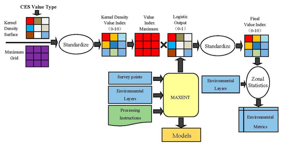
Figure 2.
The value index (VI) maps generalized key process flow.
2.3.2. SD Modelling
Each factor of CES has direct or indirect connections. Changes in one factor may influence the other factors, leading to changes throughout the whole system. SD can objectively and dynamically determine the developmental trends of different CES by mathematical modelling. Mathematical modelling can establish equations and functional relationships between factors in each subsystem of the CES. By studying the dynamic changes and developmental trends of CES, we can further understand the developmental tracks of regional CES. It is also an opportunity to explore the application of SD in different fields.
At present, the most commonly used modelling software for SD is STELLA, Vensim, Ithink, Powersim, etc. [42,43,44,45]. We chose to use Vensim DSS × 64 SD modelling software based on the research purpose and simulation requirements of this study. The Vensim SD model was used to construct a cause and effect diagram of CES in Xi’an. The variables impacting each system were determined through causality analysis. The dynamic model in this study was based on the impact strength of different variables related to CES. A system flow diagram and equation for each district were established, and a developmental track of CES in Xi’an was simulated. The developmental trends of ecosystem culture in Xi’an were used to predict and simulate future scenarios. The established subsystems included population, economics, and culture. Meanings of different variable names are shown in Table A1 of Appendix A. The various equations in SD model are shown in Table 4.
Table 4.
Key equations in SD Model.
(1) Population influences the economics and environment of cities through aspects such as labor force, consumption of entertainment, and tourist recreation [46,47]. Population changes are also based on feedback principles and are influenced by economic development, environmental changes, and urban CES [48].
(2) Economic activity is a consequential part of daily human life. GDP is an important measure of economic development and can directly reflect the degree and level of economic development in a region [32]. When a regional cultural service is promoted, it develops regional tourism, the entertainment industry, and the catering and accommodation industries, thus feeding back into the economy and further promoting economic development [49].
(3) Based on Xi’an’s characteristics, aesthetics, history, and entertainment were selected as determinates of culture in our SD modelling. The CES subsystem mainly aims to show the relationship between various values and the corresponding main influencing factors. By analyzing the characteristics of the value distributions of these three CES, it was determined that the degree of urbanization has the greatest influence on historical value, the distance from roads and water have the greatest influence on aesthetic value, and the opportunities for recreational activities and area of green space have the greatest impact on the entertainment value. Pollution of the air and water causes a reduction in spontaneous recreational activities, and therefore should be included in the system variables [50]. Economic investment in different CES can also have a crucial impact on CES [47,51].
The study included a population subsystem, an economic subsystem, and a cultural services subsystem. The total system flow diagram of the entire SD model was formed by connecting subsystems with each other using a series of common variables, as shown in Figure 3.
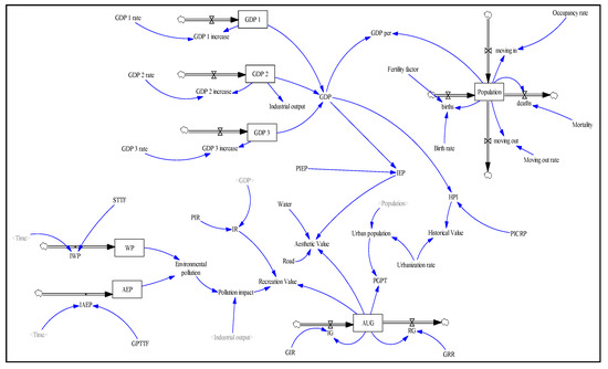
Figure 3.
Flow chat of the total system.
2.3.3. Future Development Scenarios
Four scenarios for the future development of Xi’an were set up in order to simulate and predict dynamic changes to CES in 2030. The four scenarios were a natural development scenario (NAD), an environmental protection scenario (ENP), an economic priority scenario (ECP), and a coordinated development scenario (COD). In the NAD, we assumed that each region will continue to develop according to the existing trends, and the average values from 2014 to 2017 were used as variable parameters. In the ENP, we set the economic growth rate lower (a minimum value of about 2014 to 2017) and the developmental speed of regional green land and gardens higher (a maximum value of about 2014 to 2017), reflecting the impact of tertiary industry. The value added in the tertiary industry was set to average. In the ECP, we set the economic growth rate higher (maximum value of about 2014 to 2017) and the developmental speed of regional green land and gardens lower (minimum value of about 2014 to 2017). In the COD, we set each region’s economic growth rate and regional green land and garden development rate to more balanced levels; that is, the rate of increase of green space areas and other economic variable parameters were set to a higher value of 2014 to 2017. The parameter settings for different scenarios are shown in Table A2, Table A3, Table A4 and Table A5 of Appendix A.
3. Results
3.1. CES Distribution Status and Principle
The distributions of CES in Xi’an are shown in Figure 4. High recreation value areas were around the roads and radiated outward to the surrounding areas. Hot spots are formed in areas near rivers and green spaces. The radiation range of recreation value is less than aesthetic value but higher than historical value on the road and the surrounding area at the junction of Xi’an City and Qinling Mountains.
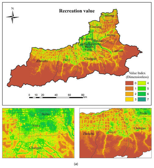
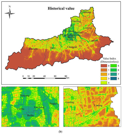
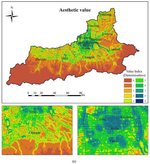
Figure 4.
The VI map of CES. (a) Recreation VI map. (b) Historical VI map. (c) Aesthetic VI map.
Areas with high historical value were more extensive and were distributed more densely in urban areas compared with areas of aesthetic value. Further, the ranges of historical value radiating from the roads and nearby areas were more extensive than aesthetic value. However, there were no high value points in some of the water and green areas.
Denser high-value areas of aesthetic value were concentrated in the main urban areas. The aesthetic value is high in the vicinity of roads, water and green areas. The southern part of Xi’an, a junction with the northern foot of the Qinling Mountains, was a cold spot for CES, with the only high value points distributed on roads and nearby small areas.
3.2. SD Model in Different Scenarios
After constructing a SD model of CES, set the start and end dates of the model as 2014 and 2030 respectively. The simulation step length was one year. After the model was run, the simulated values of each subsystem variable were obtained.
Under each different scenario setting, we predicted the economic, green space, and CES status in 2030. In order to better integrate the CES status of each division under different scenarios, the same weight value was given to recreation, historical, aesthetic and the total CES values were added to determine the CES development.
The economic development of each district achieved the fastest growth under the ECP. The predictions of 2030 GDP output for each administrative division were highest from the ECP, then the COD, and then the NAD, and lowest from the ENP. The changes in green space area in each district achieved the fastest increase under the ENP. The green space area values in each administrative division were predicted, by 2030, to increase the most in the ENP, then the COD, then the NAD, and least in the ECP. The predicted values of CES in 2030 are shown in Figure 5.
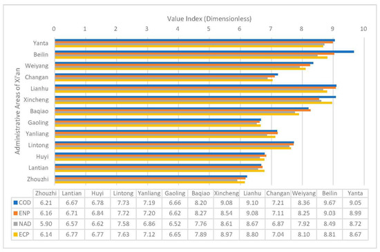
Figure 5.
The predicted values of CES in 2030.
We predicted the 2030 average values of CES, including COD, ENP, ECP, and NAD in all districts. The average values of CES in the Baqiao, Yanliang, and Huyi districts were highest for the ENP and lowest in the NAD. The average values of CES in the Lantian district was highest in the ECP and lowest in the NAD. The average values for CES in the Yanta district was highest in the COD and lowest in the ECP. The average values of CES in the Xincheng district was highest in the COD and lowest in the ENP. The average values of CES in the Zhouzhi, Lintong, Gaoling, Lianhu, Changan, Weiyang, and Beilin districts were highest in the COD and lowest in the NAD.
We found that in different districts, the COD and ENP generally predicted higher CES values, while CES values were lower under the NAD. CES values predicted by the ECP showed larger changes in different districts.
3.3. Performance of ECP in Different Districts
In order to further analyze the CES in different districts and under different scenarios, we calculated the difference between the ECP and other scenarios of CES, and then added the absolute values to get the CES gap between different scenarios. The CES gap is sorted from high to low in terms of GDP in Figure 6. From the Yanta district to the Zhouzhi district, predicted GDP output gradually decreased.
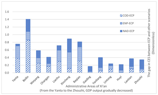
Figure 6.
The impact of the economy on different administration district.
As seen in Figure 6, as the regional GDP output value decreased, the differences in various scenarios showed a narrowing trend. In regions with high levels of regional economic development, different scenarios have a large impact on CES. However, when the level of economic development in a region is low, the differences in CES under different scenarios are small; the differences between the COD and the ECP, as well as the differences between ENP and the ECP, were significantly reduced compared with regions that have high economic development. In other words, choosing the ECP in regions with low economic development may produce similar CES results as that of the COD or ENP, while also maintaining relatively high economic growth.
4. Discussion
4.1. Environmental Index Impact Analysis
In addition to producing a VI map, the SolVES model output was also used to generate mathematical statistics comparing the relationships of CES and environmental indexes. The statistics are presented in Figure 7.
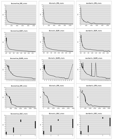
Figure 7.
The relationship between CES value and environmental index. Among the types of LULC, 1 represents grassland, 2 represents forest land, 3 represents cultivated land, 4 represents water body, 5 represents unused land, and 6 represents urban land.
Recreation value is negatively correlated with DTR, DTW, ELEV, SLOPE, and other environmental indexes. As the distance from roads and water increases, the elevation and slope increase, which cause a downward trend in recreation value. Forest land and cultivated land can provide recreation value. Water and urban land can provide higher recreation value.
Historical value is negatively correlated with environmental indexes such as DTR, DTW, and ELEV. As the distance from roads and water increases, the elevation causes the historical value to display a downward trend. The slope statistics first decline and then increase. This may be due to the fact that some temples, including Taoist temples, are located near the foot of Qinling Mountains, thus increasing historical value in some areas with higher slopes. Forest land and cultivated land can both provide historical value. Cultivated land provides higher historical value than forest land. Urban land can also provide high historical value.
Aesthetic value is negatively correlated with DTR, DTW, ELEV, SLOPE, and other environmental indexes. As the distance from the road or water increased, the elevation and slope of the elevation caused a downward trend in the aesthetic value. There is some fluctuation in the slope statistics, but the overall trend is downward. This may be due to the green space and woodlands located on both sides of the river and in front of the mountain, which can provide higher aesthetic value. Forest land and cultivated land can provide aesthetic value, while urban land can provide higher aesthetic value.
4.2. Analysis of CES Distribution Characteristics
Places that have more opportunities for recreational activities, such as areas near water bodies and green spaces in city parks will form hot spots, which are areas that people think have high recreation value. Some indoor entertainment facilities and places in the city center also provide a lot of entertainment opportunities, so they are also considered to be of high recreation value. Although the southern area near the Qinling Mountains has been gradually developed in recent years, such as a series of summer resorts, there are still relatively few opportunities and places for recreation activities and high transportation costs, so it has not been considered to have entertainment value.
The high value areas of historical value are widely distributed because Xi’an has thousands of years of capital history, and there are countless places of interest, tombs, and so on. Some of these have become well-known historical tourist attractions in China and abroad. Some newly built water bodies and green spaces will not be considered as having historical value. In areas with frequent human activities, the urban areas where the urban settlements originated earlier will be considered to have high historical value.
The locations of hot spots with aesthetic value formed in urban areas are mostly consistent with tourist attractions, forest parks and urban green space parks, such as Daming Palace National Heritage Park and Weiyang Lake in Weiyang; Qujiangchi Heritage Park and Tang Paradise in Yanta; Zhongnan Mountain Ancient Building in Zhouzhi; Lishan Mountain in Lintong; Cuihua Mountain Forest Park and Xi’an Qinling Wilding Zoo in Chang’an—these areas have high aesthetic value. There are many famous tourist attractions in the inner city of Xi’an, such as the Bell Tower, the Drum Tower, the Forest of Steles, and the Muslim’s Quarter, etc., which correspond to the large range of high-value areas within the city wall area.
There are many forest parks in Zhouzhi, Chang’an, Wuyi, Lantian, and other areas near the northern of Qinling Mountains, such as Heihe National Forest Park, Zhuque National Forest Park, Golden monkey nature reserve, etc. Although these areas have beautiful scenery and high forest coverage, the terrain near the Qinling Mountains is relatively steep, the distance relatively far from urban areas, and the elevation increases significantly. Only high value points will be formed on roads and nearby areas. Its own aesthetic value has not been fully detected and well known to the public. In summary, the areas with convenient transportation, more well-known scenic spots and covered by green land and water will be considered to have high aesthetic value. However, some areas far away from people’s living areas with steep terrain and less convenient transportation cannot be considered to have corresponding aesthetic value.
A research found that most of the respondents in Gaoqu Town, Shaanxi Province acknowledged the aesthetic services of woodlands and grasslands. They consider aesthetic service is of the highest value in the Town [52]. In Guyuan, Ningxia Hui Autonomous Region, northern China, scholars have found that cultivated land is regarded as a significant land-use provider for CES [53]. Forests and large parks play major roles in providing CES [54]. These services of aesthetic beauty, the opportunity for leisure activities are mainly attributed to the intensive use of meadows and forests. In contrast, cultural heritage is primarily perceived in landscapes with strong man-made influences, such as villages [55]. SolVES has been applied to conduct CES assessment of a wetland forest park in Shanghai and the results showed that the field of view was broad and that the area adjacent to the water source had higher cultural service values [56]. Those results of other scholars’ research on CES are consistent with the results obtained in this study.
4.3. Limitations
This research still has some limitations. Many factors in the SolVES model, such as investigation time and manpower, may have various biases caused by the composition of the respondent population, the number of regional survey respondents, and other factors. To improve the accuracy of the survey data, studies should be run over a longer time, include a larger area, and collect multiple samples to investigate and prevent deviations. Furthermore, the SolVES model uses the same environmental index for different landscape types, which can cause errors.
Our dynamic model of CES was based on the available data sources and we selected the relevant variables to use in the model. However, in fact, our research is limited by data collection and quantification methods and cannot be modeled and considered for all variables because the factors affecting CES are diverse and interact with each other. For example, there are other factors such as inflation and industrial growth rate that can affect GDP. The model could be improved by future insights into how to accurately select the most suitable influencing factors and determine the relationships between the different factors. Secondly, the future simulation research requires to be corrected for a long time with the actual situation. With the development of Xi’an’s tourism industry, the ratio of economic benefits of tourism industry to GDP is gradually increasing. At present, it is showing a trend of growth, so the future simulation research still requires to be corrected by observing the actual GDP ratio year by year for a long time.
4.4. Future Development Management
With the decline of regional economic level, the differences in CES between various scenarios are shrinking. In areas with high levels of economic development, the impact on different scenarios of CES is quite different. However, when the economic development level of a region is low, the differences in CES in various scenarios are smaller. Other studies found that when people face more survival risks, their perception of the surrounding CES will be reduced [57]. People’s direct experience plays an important role in shaping their perception of the surrounding CES [58]. CES can be evaluated after they are perceived. For the local residents, regional economic development is backward, people may be more focused on raising a family, and when the regional economy is further developed, people no longer have great pressure to live, and may enjoy the surrounding scenery more. For tourists, when the regional economy is relatively backward, the infrastructure is not perfect, tourism publicity is not strong enough to attract tourists [59]. As economic development brings increased publicity, more CES are bound to be perceived by tourists.
Based on this, different administrative divisions should have their own positions in the future development and they should be comprehensively considered according to their own development priorities and characteristics to choose a development strategy suitable for the region. In regions with low economic development level, priority can be given to economic development and people’s living standards can be improved. Attention also should be paid to the protection of ecological environment, so as to improve the economic level and CES at the same time. In order to realize the sustainable development in the future, the regions with more developed economy should devote themselves to the protection and construction of ecological environment and accelerate the transformation of traditional industries.
5. Conclusions
In this paper, social survey data and environmental index data were obtained through field investigation and used to calculate VI maps for recreation, historical, and aesthetic services in Xi’an using the SolVES model. Based on our analysis of the factors associated with various CES values, the components and boundaries of each CES subsystem were defined and a system flow diagram between each of the factors were plotted. We used the Vensim DSS x 64 model to establish a SD model of the CES system in various districts in Xi’an. Four different development scenarios (natural development, environmental protection, economic priority, and coordinated development) were used to predict the dynamic changes of CES in 2030. When the level of economic development in a region is low, the differences in CES under different scenarios are small; the differences between scenarios were significantly reduced compared with regions that have high economic development. We found that different development scenarios were most applicable to different regions and that each region needs to choose according to their future developmental directions to achieve their corresponding developmental needs.
Author Contributions
Q.Z. and J.L. designed the study. Q.Z. and Y.C. performed the field survey and data analysis. Z.Z. provided advice on the conclusions and research prospect, and edited the English language. Q.Z. wrote the paper with contributions from all authors. All authors have read and agreed to the published version of the manuscript.
Funding
This research was funded by the National Natural Science Foundation of China, No. 41771198, No. 41771576; The NSFC-NRF Scientific Cooperation Program (Grant no. 41811540400). And The Project Supported by Natural Science Basic Research Plan in Shaanxi Province of China (Program No. 2018JM4010). The Fundamental Research Funds for the Central Universities, Shaanxi Normal University (GK201901009).
Acknowledgments
We are grateful to anonymous reviewers and members of the editorial team for advice.
Conflicts of Interest
The authors declare no conflict of interest.
Appendix A
Table A1.
Meaning of Variable name in SD.
Table A1.
Meaning of Variable name in SD.
| Variable Name | Meaning |
|---|---|
| GDP 1 rate | Growth rate of value added in primary industry |
| GDP 1 increase | Increase in value added in primary industry |
| GDP 1 | Value added in primary industry |
| GDP 2 rate | Growth rate of value added in secondary industry |
| GDP 2 increase | Increase in value added in secondary industry |
| GDP 2 | Value added in the secondary industry |
| GDP 3 rate | Growth rate of value added in the tertiary industry |
| GDP 3 increase | Value added growth in the tertiary industry |
| GDP 3 | Value added in the tertiary industry |
| Industrial output | Industrial output |
| GDP | GDP |
| GDP per | GDP per capita |
| Population | Population |
| births | Number of births in the year |
| Fertility factor | Fertility factor |
| Birth rate | Birth rate |
| moving out | Number of moving out in the year |
| Moving out rate | Moving out rate |
| deaths | Number of deaths in the year |
| Mortality | Mortality |
| moving in | Number of moving in in the year |
| Occupancy rate | Occupancy rate |
| PIEP | Percentage of investment in environmental protection |
| IEP | Investment in environmental protection |
| Water | Water |
| Road | Road |
| Aesthetic Value | Aesthetic Value |
| PIR | Percentage of investment in Recreation |
| IR | Investment in Recreation |
| IWP | Increase in water pollution |
| WP | Water pollution |
| IAEP | Increase in atmospheric environmental pollution |
| AEP | atmospheric environmental pollution |
| STTF | Sewage treatment technology factors |
| GPTTF | Gas pollution treatment technology factors |
| Environmental pollution | Environmental pollution |
| Pollution impact | Pollution impact |
| Recreation Value | Recreation Value |
| GIR | Greenfield increase rate |
| IG | Increase in Greenfield |
| AUG | Area of urban Greenfield |
| RG | Reduction in Greenfield |
| GRR | Greenfield reduction rate |
| PGPT | Public Greenfield per capita in towns |
| Urban population | Urban population |
| Urbanization rate | Urbanization rate |
| HPI | Heritage protection investment |
| PICRP | Percentage of investment in cultural relics protection |
| Historical Value | Historical Value |
Table A2.
Parameter setting of natural development scenario.
Table A2.
Parameter setting of natural development scenario.
| Districts | GDP 1 Rate | GDP 2 Rate | GDP 3 Rate | GIR |
|---|---|---|---|---|
| Xincheng | 0 | 0.04 | 0.12 | 0.0238 |
| Beilin | 0 | 0.17 | 0.12 | 0.03 |
| Lianhu | 0 | 0.1 | 0.135 | 0.03 |
| Baqiao | 0.0669 | 0.007 | 0.198 | 0.033 |
| Weiyang | −0.143 | 0.072 | 0.104 | 0.0668 |
| Yanta | 0 | −0.008 | 0.171 | 0.0315 |
| Yanliang | 0.045 | 0.06 | 0.19 | 0.0279 |
| Lintong | 0.0132 | −0.127 | 0.164 | 0.0267 |
| Changan | 0.02 | 0.265 | 0.2 | 0.04 |
| Zhouzhi | 0.066 | 0.058 | 0.156 | 0.04 |
| Huyi | 0.024 | 0.052 | 0.145 | 0.2 |
| Lantian | 0.0543 | 0.0375 | 0.145 | 0.253 |
| Gaoling | 0.103 | 0.045 | 0.197 | 0.14 |
Table A3.
Parameter setting of environmental protection scenario.
Table A3.
Parameter setting of environmental protection scenario.
| Districts | GDP 1 Rate | GDP 2 Rate | GDP 3 Rate | GIR |
|---|---|---|---|---|
| Xincheng | 0 | 0.08 | 0.08 | 0.06 |
| Beilin | 0 | 0.1 | 0.12 | 0.05 |
| Lianhu | 0 | 0.03 | 0.135 | 0.04 |
| Baqiao | 0.005 | 0.001 | 0.15 | 0.04 |
| Weiyang | −0.3 | 0.04 | 0.1 | 0.2 |
| Yanta | 0 | −0.07 | 0.1 | 0.04 |
| Yanliang | 0.003 | 0.01 | 0.14 | 0.04 |
| Lintong | 0.01 | −0.3 | 0.1 | 0.04 |
| Changan | 0.01 | 0.2 | 0.2 | 0.06 |
| Zhouzhi | 0.02 | 0.03 | 0.1 | 0.2 |
| Huyi | 0.01 | 0.02 | 0.1 | 0.4 |
| Lantian | 0.004 | 0.01 | 0.14 | 0.4 |
| Gaoling | 0.03 | 0.02 | 0.1 | 0.3 |
Table A4.
Parameter setting of economic priority scenario.
Table A4.
Parameter setting of economic priority scenario.
| Districts | GDP 1 Rate | GDP 2 Rate | GDP 3 Rate | GIR |
|---|---|---|---|---|
| Xincheng | 0 | 0.18 | 0.28 | 0.002 |
| Beilin | 0 | 0.3 | 0.2 | 0.015 |
| Lianhu | 0 | 0.23 | 0.3 | 0.01 |
| Baqiao | 0.1 | 0.2 | 0.41 | 0.01 |
| Weiyang | −0.1 | 0.2 | 0.2 | 0.03 |
| Yanta | 0 | −0.004 | 0.35 | 0.01 |
| Yanliang | 0.1 | 0.2 | 0.43 | 0.02 |
| Lintong | 0.04 | −0.06 | 0.32 | 0.01 |
| Changan | 0.1 | 0.4 | 0.5 | 0.01 |
| Zhouzhi | 0.2 | 0.2 | 0.3 | 0.007 |
| Huyi | 0.07 | 0.3 | 0.25 | 0.08 |
| Lantian | 0.1 | 0.15 | 0.25 | 0.1 |
| Gaoling | 0.2 | 0.22 | 0.45 | 0.08 |
Table A5.
Parameter setting of coordinated development scenario.
Table A5.
Parameter setting of coordinated development scenario.
| Districts | GDP 1 Rate | GDP 2 Rate | GDP 3 Rate | GIR |
|---|---|---|---|---|
| Xincheng | 0 | 0.12 | 0.21 | 0.04 |
| Beilin | 0 | 0.2 | 0.16 | 0.04 |
| Lianhu | 0 | 0.15 | 0.17 | 0.035 |
| Baqiao | 0.08 | 0.15 | 0.3 | 0.035 |
| Weiyang | −0.15 | 0.15 | 0.15 | 0.15 |
| Yanta | 0 | −0.006 | 0.25 | 0.035 |
| Yanliang | 0.075 | 0.15 | 0.3 | 0.035 |
| Lintong | 0.03 | −0.12 | 0.25 | 0.034 |
| Changan | 0.08 | 0.35 | 0.4 | 0.05 |
| Zhouzhi | 0.15 | 0.15 | 0.2 | 0.15 |
| Huyi | 0.06 | 0.15 | 0.2 | 0.3 |
| Lantian | 0.08 | 0.1 | 0.2 | 0.3 |
| Gaoling | 0.1 | 0.1 | 0.32 | 0.25 |
References
- Costanza, R.; dArge, R.; deGroot, R.; Farber, S.; Grasso, M.; Hannon, B.; Limburg, K.; Naeem, S.; Oneill, R.V.; Paruelo, J.; et al. The value of the world’s ecosystem services and natural capital. Nature 1997, 387, 253–260. [Google Scholar] [CrossRef]
- Daily, G.C.; Polasky, S.; Goldstein, J.; Kareiva, P.M.; Mooney, H.A.; Pejchar, L.; Ricketts, T.H.; Salzman, J.; Shallenberger, R. Ecosystem services in decision making: Time to deliver. Front. Ecol. Environ. 2009, 7, 21–28. [Google Scholar] [CrossRef]
- Hooper, D.U.; Chapin, F.S.; Ewel, J.J.; Hector, A.; Inchausti, P.; Lavorel, S.; Lawton, J.H.; Lodge, D.M.; Loreau, M.; Naeem, S.; et al. Effects of biodiversity on ecosystem functioning: A consensus of current knowledge. Ecol. Monogr. 2005, 75, 3–35. [Google Scholar] [CrossRef]
- Costanza, R.; de Groot, R.; Sutton, P.; van der Ploeg, S.; Anderson, S.J.; Kubiszewski, I.; Farber, S.; Turner, R.K. Changes in the global value of ecosystem services. Glob. Environ. Chang.-Hum. Policy Dimens. 2014, 26, 152–158. [Google Scholar] [CrossRef]
- Carpenter, S.R.; Mooney, H.A.; Agard, J.; Capistrano, D.; DeFries, R.S.; Diaz, S.; Dietz, T.; Duraiappah, A.K.; Oteng-Yeboah, A.; Pereira, H.M.; et al. Science for managing ecosystem services: Beyond the Millennium Ecosystem Assessment. Proc. Natl. Acad. Sci. USA 2009, 106, 1305–1312. [Google Scholar] [CrossRef] [PubMed]
- Brown, G.; Pullar, D.; Hausner, V.H. An empirical evaluation of spatial value transfer methods for identifying cultural ecosystem services. Ecol. Indic. 2016, 69, 1–11. [Google Scholar] [CrossRef]
- Reyers, B.; Biggs, R.; Cumming, G.S.; Elmqvist, T.; Hejnowicz, A.P.; Polasky, S. Getting the measure of ecosystem services: A social-ecological approach. Front. Ecol. Environ. 2013, 11, 268–273. [Google Scholar] [CrossRef]
- Cheng, X.; Van Damme, S.; Li, L.; Uyttenhove, P. Evaluation of cultural ecosystem services: A review of methods. Ecosyst. Serv. 2019, 37, 100925. [Google Scholar] [CrossRef]
- Johansson, M.; Pedersen, E.; Weisner, S. Assessing cultural ecosystem services as individuals’ place-based appraisals. Urban For. Urban Green. 2019, 39, 79–88. [Google Scholar] [CrossRef]
- Retka, J.; Jepson, P.; Ladle, R.J.; Malhado, A.C.M.; Vieira, F.A.S.; Normande, I.C.; Souza, C.N.; Bragagnolo, C.; Correia, R.A. Assessing cultural ecosystem services of a large marine protected area through social media photographs. Ocean Coast. Manag. 2019, 176, 40–48. [Google Scholar] [CrossRef]
- Jaligot, R.; Kemajou, A.; Chenal, J. Cultural ecosystem services provision in response to urbanization in Cameroon. Land Use Policy 2018, 79, 641–649. [Google Scholar] [CrossRef]
- Junge, X.; Schuepbach, B.; Walter, T.; Schmid, B.; Lindemann-Matthies, P. Aesthetic quality of agricultural landscape elements in different seasonal stages in Switzerland. Landsc. Urban Plan. 2015, 133, 67–77. [Google Scholar] [CrossRef]
- Oteros-Rozas, E.; Martin-Lopez, B.; Fagerholm, N.; Bieling, C.; Plieninger, T. Using social media photos to explore the relation between cultural ecosystem services and landscape features across five European sites. Ecol. Indic. 2018, 94, 74–86. [Google Scholar] [CrossRef]
- Richards, D.R.; Friess, D.A. A rapid indicator of cultural ecosystem service usage at a fine spatial scale: Content analysis of social media photographs. Ecol. Indic. 2015, 53, 187–195. [Google Scholar] [CrossRef]
- Richards, D.R.; Tuncer, B. Using image recognition to automate assessment of cultural ecosystem services from social media photographs. Ecosyst. Serv. 2018, 31, 318–325. [Google Scholar] [CrossRef]
- Paracchini, M.L.; Zulian, G.; Kopperoinen, L.; Maes, J.; Schägner, J.P.; Termansen, M.; Zandersen, M.; Perez-Soba, M.; Scholefield, P.A.; Bidoglio, G. Mapping cultural ecosystem services: A framework to assess the potential for outdoor recreation across the EU. Ecol. Indic. 2014, 45, 371–385. [Google Scholar] [CrossRef]
- Zulian, G.; Paracchini, M.L.; Maes, J.; Liquete, C. ESTIMAP: Ecosystem Services Mapping at European Scale; Publications Office of the European Union: Luxembourg, 2013. [Google Scholar] [CrossRef]
- Zulian, G.; Stange, E.; Woods, H.; Carvalho, L.; Dick, J.; Andrews, C.; Baro, F.; Vizcaino, P.; Barton, D.N.; Nowel, M.; et al. Practical application of spatial ecosystem service models to aid decision support. Ecosyst Serv 2018, 29, 465–480. [Google Scholar] [CrossRef] [PubMed]
- Burkhard, B.; Kroll, F.; Nedkov, S.; Mueller, F. Mapping ecosystem service supply, demand and budgets. Ecol. Indic. 2012, 21, 17–29. [Google Scholar] [CrossRef]
- Brunina, L.; Konstantinova, E.; Persevica, A.; Rezekne Higher Educ, I. Necessity of Mapping and Assessment of Ecosystems and Their Services in Planning and Decision Making Process. 2016. Available online: https://c3cc7c618ee75efbd177329691486ef3enll.casb.nju.edu.cn:4443/index.php/SIE/article/view/1573 (accessed on 28 May 2016).
- Sharp, J. System dynamics and system dynamic application-reply. J. Oper. Res. Soc. 1978, 29, 507–508. [Google Scholar] [CrossRef]
- Martinez-Jaramillo, J.E.; Arango-Aramburo, S.; Giraldo-Ramirez, D.P. The effects of biofuels on food security: A system dynamics approach for the Colombian case. Sustain. Energy Technol. Assess. 2019, 34, 97–109. [Google Scholar] [CrossRef]
- Morii, Y.; Ishikawa, T.; Suzuki, T.; Tsuji, S.; Yamanaka, M.; Ogasawara, K.; Yamashina, H. Projecting future supply and demand for physical therapists in Japan using system dynamics. Health Policy Technol. 2019, 8, 118–127. [Google Scholar] [CrossRef]
- Tegegne, W.A.; Moyle, B.D.; Becken, S. A qualitative system dynamics approach to understanding destination image. J. Destin. Mark. Manag. 2018, 8, 14–22. [Google Scholar] [CrossRef]
- Xu, J.; Kang, J.; Shao, L.; Zhao, T. System dynamic modelling of industrial growth and landscape ecology in China. J. Environ. Manag. 2015, 161, 92–105. [Google Scholar] [CrossRef] [PubMed]
- Xu, Z.; Coors, V. Combining system dynamics model, GIS and 3D visualization in sustainability assessment of urban residential development. Build. Environ. 2012, 47, 272–287. [Google Scholar] [CrossRef]
- You, S.; Kim, M.; Lee, J.; Chon, J. Coastal landscape planning for improving the value of ecosystem services in coastal areas: Using system dynamics model. Environ. Pollut. 2018, 242, 2040–2050. [Google Scholar] [CrossRef] [PubMed]
- Jaligot, R.; Chenal, J.; Bosch, M.; Hasler, S. Historical dynamics of ecosystem services and land management policies in Switzerland. Ecol. Indic. 2019, 101, 81–90. [Google Scholar] [CrossRef]
- Wu, M.; Ren, X.; Che, Y.; Yang, K. A Coupled SD and CLUE-S Model for Exploring the Impact of Land Use Change on Ecosystem Service Value: A Case Study in Baoshan District, Shanghai, China. Environ. Manag. 2015, 56, 402–419. [Google Scholar] [CrossRef]
- Chen, H.; Chang, Y.C.; Chen, K.C. Integrated wetland management: An analysis with group model building based on system dynamics model. J. Environ. Manag. 2014, 146, 309–319. [Google Scholar] [CrossRef]
- Lu, S.S.; Qin, F.; Chen, N.; Yu, Z.Y.; Xiao, Y.M.; Cheng, X.Q.; Guan, X.L. Spatiotemporal differences in forest ecological security warning values in Beijing: Using an integrated evaluation index system and system dynamics model. Ecol. Indic. 2019, 104, 549–558. [Google Scholar] [CrossRef]
- Cordier, M.; Uehara, T.; Weih, J.; Hamaide, B. An Input-output Economic Model Integrated within a System Dynamics Ecological Model: Feedback Loop Methodology Applied to Fish Nursery Restoration. Ecol. Econ. 2017, 140, 46–57. [Google Scholar] [CrossRef]
- Elliot, T.; Babí Almenar, J.; Niza, S.; Proença, V.; Rugani, B. Pathways to Modelling Ecosystem Services within an Urban Metabolism Framework. Sustainability 2019, 11, 2766. [Google Scholar] [CrossRef]
- Lopes, R.; Videira, N. Modelling feedback processes underpinning management of ecosystem services: The role of participatory systems mapping. Ecosyst. Serv. 2017, 28, 28–42. [Google Scholar] [CrossRef]
- Aspinall, R.; Staiano, M. Ecosystem services as the products of land system dynamics: Lessons from a longitudinal study of coupled human–environment systems. Landsc. Ecol. 2018, 34, 1503–1524. [Google Scholar] [CrossRef]
- Boumans, R.; Roman, J.; Altman, I.; Kaufman, L. The Multiscale Integrated Model of Ecosystem Services (MIMES): Simulating the interactions of coupled human and natural systems. Ecosyst. Serv. 2015, 12, 30–41. [Google Scholar] [CrossRef]
- Zhai, B.; Ng, M.K. Urban regeneration and social capital in China: A case study of the Drum Tower Muslim District in Xi’an. Cities 2013, 35, 14–25. [Google Scholar] [CrossRef]
- Qian, Z.; Li, H. Urban morphology and local citizens in China’s historic neighborhoods: A case study of the Stele Forest Neighborhood in Xi’an. Cities 2017, 71, 97–109. [Google Scholar] [CrossRef]
- Brown, G.; Brabyn, L. An analysis of the relationships between multiple values and physical landscapes at a regional scale using public participation GIS and landscape character classification. Landsc. Urban Plan. 2012, 107, 317–331. [Google Scholar] [CrossRef]
- van Riper, C.J.; Kyle, G.T.; Sutton, S.G.; Barnes, M.; Sherrouse, B.C. Mapping outdoor recreationists’ perceived social values for ecosystem services at Hinchinbrook Island National Park, Australia. Appl. Geogr. 2012, 35, 164–173. [Google Scholar] [CrossRef]
- Liu, J.; Li, J.; Qin, K.; Zhou, Z.; Yang, X.; Li, T. Changes in land-uses and ecosystem services under multi-scenarios simulation. Sci. Total Environ. 2017, 586, 522–526. [Google Scholar] [CrossRef]
- Walters, J.P.; Archer, D.W.; Sassenrath, G.F.; Hendrickson, J.R.; Hanson, J.D.; Halloran, J.M.; Vadas, P.; Alarcon, V.J. Exploring agricultural production systems and their fundamental components with system dynamics modelling. Ecol. Model. 2016, 333, 51–65. [Google Scholar] [CrossRef]
- Spicar, R. System Dynamics Archetypes in Capacity Planning. 2014. Available online: https://elkssl0a75e822c6f3334851117f8769a30e1celksslscience.casb.nju.edu.cn:4443/10.1016/j.proeng.2014.03.128 (accessed on 12 March 2014).
- Morcillo, J.D.; Franco, C.J.; Angulo, F. Simulation of demand growth scenarios in the Colombian electricity market: An integration of system dynamics and dynamic systems. Appl. Energy 2018, 216, 504–520. [Google Scholar] [CrossRef]
- Bautista, S.; Espinoza, A.; Narvaez, P.; Camargo, M.; Morel, L. A system dynamics approach for sustainability assessment of biodiesel production in Colombia. Baseline simulation. J. Clean. Prod. 2019, 213, 1–20. [Google Scholar] [CrossRef]
- Ravar, Z.; Zahraie, B.; Sharifinejad, A.; Gozini, H.; Jafari, S. System dynamics modeling for assessment of water-food-energy resources security and nexus in Gavkhuni basin in Iran. Ecol. Indic. 2020, 108, 18. [Google Scholar] [CrossRef]
- Wan, L.H.; Zhang, Y.W.; Qi, S.Q.; Li, H.Y.; Chen, X.H.; Zang, S.Y. A study of regional sustainable development based on GIS/RS and SD model - Case of Hadaqi industrial corridor. J. Clean Prod. 2017, 142, 654–662. [Google Scholar] [CrossRef]
- Lyons, G.J.; Duggan, J. System dynamics modelling to support policy analysis for sustainable health care. J. Simul. 2015, 9, 129–139. [Google Scholar] [CrossRef]
- Chen, Y.F.; Qi, J.; Zhou, J.X.; Li, Y.P.; Xiao, J. Dynamic modeling of a man-land system in response to environmental catastrophe. Hum. Ecol. Risk Assess. 2004, 10, 579–593. [Google Scholar] [CrossRef]
- Pouso, S.; Borja, A.; Martin, J.; Uyarra, M.C. The capacity of estuary restoration to enhance ecosystem services: System dynamics modelling to simulate recreational fishing benefits. Estuar. Coast. Shelf Sci. 2019, 217, 226–236. [Google Scholar] [CrossRef]
- Karami, S.; Karami, E.; Buys, L.; Drogemuller, R. System dynamic simulation: A new method in social impact assessment (SIA). Environ. Impact Assess. Rev. 2017, 62, 25–34. [Google Scholar] [CrossRef]
- Shi, Q.; Chen, H.; Liang, X.; Zhang, H.; Liu, D. Cultural ecosystem services valuation and its multilevel drivers: A case study of Gaoqu Township in Shaanxi Province, China. Ecosyst. Serv. 2020, 41, 101052. [Google Scholar] [CrossRef]
- Dou, Y.; Zhen, L.; Yu, X.; Bakker, M.; Carsjens, G.J.; Xue, Z. Assessing the influences of ecological restoration on perceptions of cultural ecosystem services by residents of agricultural landscapes of western China. Sci. Total Environ. 2019, 646, 685–695. [Google Scholar] [CrossRef]
- Ko, H.; Son, Y. Perceptions of cultural ecosystem services in urban green spaces: A case study in Gwacheon, Republic of Korea. Ecol. Indic. 2018, 91, 299–306. [Google Scholar] [CrossRef]
- Zoderer, B.M.; Tasser, E.; Erb, K.-H.; Lupo Stanghellini, P.S.; Tappeiner, U. Identifying and mapping the tourists perception of cultural ecosystem services: A case study from an Alpine region. Land Use Policy 2016, 56, 251–261. [Google Scholar] [CrossRef]
- Wang, Y.; Fu, B.-T.; Lyu, Y.-P.; Yang, K.; Che, Y. Assessment of the social values of ecosystem services based on SolVES model: A case study of Wusong Paotaiwan Wetland Forest Park, Shanghai, China. Yingyong Shengtai Xuebao 2016, 27, 1767–1774. [Google Scholar] [CrossRef]
- Liu, D.; Liang, X.; Chen, H.; Zhang, H.; Mao, N. A Quantitative Assessment of Comprehensive Ecological Risk for a Loess Erosion Gully: A Case Study of Dujiashi Gully, Northern Shaanxi Province, China. Sustainability 2018, 10, 3239. [Google Scholar] [CrossRef]
- Zhang, H.; Pang, Q.; Long, H.; Zhu, H.; Gao, X.; Li, X.; Jiang, X.; Liu, K. Local Residents’ Perceptions for Ecosystem Services: A Case Study of Fenghe River Watershed. Int. J. Environ. Res. Public Health 2019, 16, 3602. [Google Scholar] [CrossRef]
- Bullock, C.; Joyce, D.; Collier, M. An exploration of the relationships between cultural ecosystem services, socio-cultural values and well-being. Ecosyst. Serv. 2018, 31, 142–152. [Google Scholar] [CrossRef]


© 2020 by the authors. Licensee MDPI, Basel, Switzerland. This article is an open access article distributed under the terms and conditions of the Creative Commons Attribution (CC BY) license (http://creativecommons.org/licenses/by/4.0/).