Abstract
We have established a stable regional geodetic reference frame using long-history (13.5 years on average) observations from 55 continuously operated Global Navigation Satellite System (GNSS) stations adjacent to the Gulf of Mexico (GOM). The regional reference frame, designated as GOM20, is aligned in origin and scale with the International GNSS Reference Frame 2014 (IGS14). The primary product from this study is the seven-parameters for transforming the Earth-Centered-Earth-Fixed (ECEF) Cartesian coordinates from IGS14 to GOM20. The frame stability of GOM20 is approximately 0.3 mm/year in the horizontal directions and 0.5 mm/year in the vertical direction. The regional reference frame can be confidently used for the time window from the 1990s to 2030 without causing positional errors larger than the accuracy of 24-h static GNSS measurements. Applications of GOM20 in delineating rapid urban subsidence, coastal subsidence and faulting, and sea-level rise are demonstrated in this article. According to this study, subsidence faster than 2 cm/year is ongoing in several major cities in central Mexico, with the most rapid subsidence reaching to 27 cm/year in Mexico City; a large portion of the Texas and Louisiana coasts are subsiding at 3 to 6.5 mm/year; the average sea-level-rise rate (with respect to GOM20) along the Gulf coast is 2.6 mm/year with a 95% confidence interval of ±1 mm/year during the past five decades. GOM20 provides a consistent platform to integrate ground deformational observations from different remote sensing techniques (e.g., GPS, InSAR, LiDAR, UAV-Photogrammetry) and ground surveys (e.g., tide gauge, leveling surveying) into a unified geodetic reference frame and enables multidisciplinary and cross-disciplinary research.
1. Introduction
The Gulf of Mexico (GOM) is located at the south end of the North American tectonic plate and north of the Caribbean plate. This region is bounded on the northeast, north and northwest by the Gulf Coast of the United States, on the southwest and south by Mexico, and on the southeast by Cuba (Figure 1). The US portion of the Gulf coastline spans approximately 2700 km crossing five states: Florida (FL), Alabama (AL), Mississippi (MS), Louisiana (LA), and Texas (TX). The Mexican portion of the Gulf coastline spans 2,805 km crossing six states: Quintana Roo, Tamaulipas, Veracruz, Tabasco, Campeche, and Yucatan. The US portion of the GOM region has been the heart of the US energy industry due to giant oil and gas reservoirs along the coast and offshore. In this study, the GOM region is bounded to the north by latitude 35°N and to the south by latitude 13°N, as depicted in Figure 1. The GOM coastal zone is defined as the contiguous area along the coast that is less than 30 meters above the global mean sea level, which is depicted as dark green in Figure 1. Some of the large cities within the coastal zone include Houston, TX; New Oreland, LA; and Miami, Tampa, FL. Much of the northern GOM coast, particularly the Mississippi River delta area of Louisiana, is sinking [1,2,3,4]. The Gulf coastal region also experiences ground deformation associated with growth faults [5,6,7,8,9].
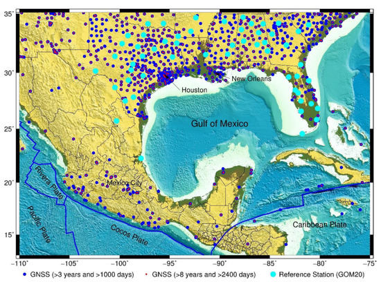
Figure 1.
Map showing Global Navigation Satellite System (GNSS) stations within the Gulf of Mexico (GOM) region. Blue dots: GNSS stations that have accumulated over 1000 daily observational files spanning over at least three years as of the end of 2019; red dots: GNSS stations that have accumulated over 2400 daily observational files spanning over at least eight years as of the end of 2019; cyan dots: 55 reference GNSS stations (average 13.5 years) for realizing the Gulf of Mexico reference frame 2020 (GOM20). The blue lines indicate plate boundaries [13]. The topographic and bathymetric datasets are from the GEBCO_2019 Grid (https://www.gebco.net).
Despite the overall tectonic stability of the GOM region, localized ground deformation associated with fault creeping and land subsidence has caused frequent damages to residential and commercial structures as well as the public infrastructure. The impacts of coastal subsidence are further exacerbated by extreme weather events (short term) and rising sea levels (long term). Rising ocean water exerts sustained impacts on coastal public infrastructure and results in coastal erosion, flooding, and wetland loss. Most of the Mississippi, Louisiana, and Texas coastline has been classified by the US Geological Survey as “highly vulnerable” to coastal erosion due to coastal subsidence and sea-level rise [10].
Coastal sea-level is often monitored by tide gauges. Tide gauge measurements are relative to nearby benchmarks fixed on land, which is historically surveyed by periodic leveling surveys and recently by Global Navigation Satellite System (GNSS) surveys. To be reproducible and comparable within a large area and over a long-time span, the benchmark and sea-level measurements must be evaluated in a well-defined and consistent frame of reference. However, the research community has difficulties in establishing a unified and consistent datum (reference frame) across the entire GOM region to evaluate long-term land deformation and sea-level changes. Different reference systems (or simply reference points) have been utilized in different areas during different periods by different researchers. Thus, it is a challenge to incorporate the published ground deformation and sea-level change results into a regional reference system. There is considerable disagreement over the rates and spatial and temporal variations of subsidence along the GOM coast, which eventually leads to controversies over the long-term impacts of coastal subsidence and sea-level rise.
A preliminary regional geodetic reference frame, named as the Stable Gulf of Mexico Reference Frame, was established in 2014 by a research group at the University of Houston [11]. The regional reference frame was realized using seven-year-long continuous observations from 13 GNSS stations adjacent to GOM. The initial reference frame was aligned to the International GNSS Service (IGS) reference frame 2008 (IGS08). IGS updated its official reference frame from IGS08 to IGS reference frame 2014 (IGS14) in 2017 [12]. GNSS stations within the GOM region have accumulated over five years of continuous observations since 2014. This study updates the initial reference frame by removing stations that are no longer in operation and adding more reference stations in order to improve the overall geographic coverage. GNSS observations, as available at the beginning of 2020, are used for realizing the regional reference frame. Accordingly, the updated reference frame is designated as GOM20. Applications of GOM20 in delineating rapid coastal subsidence, faulting, and sea-level rise are demonstrated in this article.
2. Continuous GNSS Stations within the GOM Region
Due to the inherent benefits of obtaining high-precision daily-positions using GNSS, and thereby obtaining high-accuracy displacement time series and site velocities, a dense network of Continuously Operating Reference Stations (CORS) has been established in the GOM region by the geodesy research and land surveying communities. As shown in Figure 1, there are over 1000 long-history CORS in the GOM region that each has accumulated over 1000 observational files (one file per day) spanning over at least three years as of the end of 2019. A detailed analysis of the observational history of these GNSS stations is depicted in Figure 2. Over 500 CORS have a history of over eight years and have more than 2400 daily observational files. These GNSS stations were installed and operated by the following research and surveying communities: the National Geodetic Survey (NGS) (http://geodesy.noaa.gov/CORS), UNAVCO (https://www.unavco.org/data), Texas Department of Transportation (TxDOT) (http://ftp.dot.state.tx.us), Smart Network North America (https://www.smartnetna.com), United States Coast Guard (https://www.navcen.uscg.gov), the Center for GeoInformatics Network (C4G) at the Louisiana State University (http://c4g.lsu.edu), Harris-Galveston Subsidence District (https://hgsubsidence.org), the Houston GPS Network (HoustonNet) at the University of Houston (UH), the Trans-Boundary, Land and Atmosphere Long-term Observational and Collaborative Network (TLALOCNet) in Mexico (http://cardi.geofisica.unam.mx/tlalocnet), the Continuously Operating Caribbean GPS Observational Network (COCONet) (https://coconet.unavco.org), and other local GNSS networks. Continuous GNSS datasets recorded by these networks are open to the public through the data archiving facilities at UNAVCO, National Geodetic Survey (NGS), the Crustal Dynamics Data Information System (CDDIS), and archiving sites maintained by local network operators.
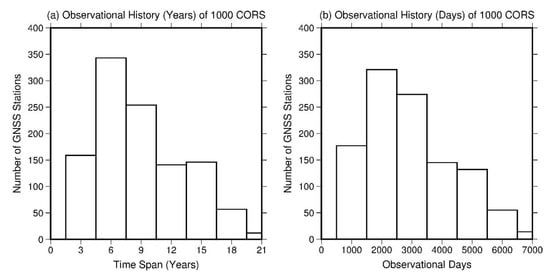
Figure 2.
Histograms illustrating the number of GNSS stations versus (a) time span (years) and (b) observational days. The total number of GNSS stations is 1000 (Figure 1).
The number of permanent GNSS stations is continuously increasing in this region. These long-term permanent GNSS stations have provided fundamental datasets for delineating ground deformation associated with faulting and subsidence within the GOM region. The majority of GNSS antennas utilized in this study are mounted on building-based monuments. Recent investigations have confirmed that long-term (e.g., >3 years) building-based GNSS monuments could provide reliable site velocity estimates for ground deformation studies provided that the buildings are stable [14,15].
This study applied the precise point positioning (PPP) method employed by the GipsyX (Version 1.2) software package (https://gipsy-oasis.jpl.nasa.gov) for calculating single-receive phase-ambiguity-fixed daily solutions with respect to IGS14. The methodology and algorithms used for the PPP solutions are described in Zumberge et al. [16] and Bertiger et al. [17]. The Nevada Geodetic Laboratory at the University of Nevada, Reno, provides daily PPP positions from over 17,000 GNSS stations to the public [18]. The Geodetic Facility for the Advancement of Geoscience (GAGE), operated by UNAVCO, also provides daily PPP solutions of numerous GNSS stations to the public [19]. The PPP method has attracted broad interests in ground deformation and structural health monitoring [20,21,22,23].
3. Realization of GOM20
GNSS positions are initially provided as a set of coordinates with respect to a global geodetic reference frame, such as IGS14, which is based on the International Terrestrial Reference Frame 2014 (ITRF14) [24]. In general, a global geodetic reference frame is a no-net-rotation (NNR) reference frame that is realized with an approach of minimizing the overall horizontal movements of a group of selected reference stations distributed worldwide [12]. As a result, GNSS-derived site movements with respect to a global reference frame are often dominated by factors such as the long-term drift and rotation of the tectonic plate on which the site is located and other secular movements [25]. In general, site velocities with respect to a global reference frame are difficult to interpret visually from a regional or local-scale geophysical perspective. Localized and/or temporal ground deformation, such as subsidence and fault creeping, could be obscured or biased by those common motions. A regional- or local-scale reference frame that fixed on the stable portion of a tectonic plate is needed when local-scale ground deformation is of interest to researchers.
There has been a conscious need for a consistent and stable reference frame in the GOM region since the early 2000s due to the rapid increase of publicly available GNSS data for the research community as well as the broad extent of land subsidence within the GOM region. During the past two decades, Interferometric Synthetic Aperture Radar (InSAR), light detection and range (LiDAR), and Unmanned Aerial Vehicle (UAV) photogrammetry techniques have also been frequently employed for mapping land subsidence, faulting, and coastal erosion within the GOM region [8,26,27,28,29,30]. Applications of remote sensing techniques further prompted the need for a unified reference frame to align measurements from different remote sensing systems.
3.1. Reference Stations
The accuracy of GNSS-derived long-term site velocities does not solely rely on equipment (antennas and receivers), but largely depends on the available regional geodetic infrastructure, which can be defined by two fundamental components: a dense continuous long-history GPS network and a stable regional reference frame [11]. The former is referred to as the hardware component, and the latter is referred to as the firmware component of a regional geodetic infrastructure. In the surveying and geodesy community, a regional reference frame is often developed through a simultaneous Helmert transformation from a well-established and broadly used global reference frame. A group of common points (reference stations), are used to link these two reference frames. The key principle for selecting a group of reference stations is that these reference stations are not expected to move relative to each other.
The selection of reference stations is critically crucial for realizing a stable reference frame. A reference station that is not locally stable will degrade the accuracy (stability) of the reference frame. Unfortunately, there are no fixed criteria for selecting reference stations. In practice, the selection is largely based on the availability of long-term GNSS stations in the study area. A stable reference frame is a secular reference frame that applies a linear motion model predicting station positions within a temporal window of interest. Therefore, the linearity of the displacement time series, which indicates how well their daily positions can be described by a constant velocity, is the key criterion for selecting reference stations. Additionally, geographic distribution, time span, data continuity, and site stability are considered for selecting reference stations. The primary criteria for selecting reference stations for realizing GOM20 include:
- (1)
- distance within 500 km to the GOM coastline;
- (2)
- having over 2400 daily files and spanning over at least eight years;
- (3)
- active through 2019 with a continuous segment of minimum 5 years;
- (4)
- outside of known subsiding or fault-creeping areas.
The vertical displacement time series with respect to IGS14 provides a quick clue to exclude those potential subsiding stations. According to our previous investigations [31,32], within the southern portion of the North American plate, a GNSS site that is not affected by localized subsidence retains a vertical site velocity well below 3 mm/year with respect to IGS global reference frames (e.g., IGS08, IGS14). In other words, if a GNSS station depicts a steady downward movement larger than 3 mm/year with respect to IGS14, this site can be confidently described as experiencing localized subsidence. Applying the four aforementioned selection criteria resulted in approximately 200 remaining candidate frame stations. Further manual screening weeded out about 100 stations with visible issues, such as frequent data gaps, significant positional shifts, and unusually large seasonal variations.
A seven-parameter transformation method was employed to realize an interim reference frame with these 100 candidate reference stations. The process for realizing a regional reference frame will be addressed in the next section. The three-component velocities of these reference stations with respect to the interim reference frame were calculated. Ideally, a stable site retains near-zero (e.g., sub-millimeter per year) three-component site velocities with respect to the stable reference frame. Reference stations with a horizontal velocity larger than 2 mm/year and a vertical velocity larger than 3 mm/year with respect to the interim reference frame were excluded as outliers. The first iteration removed 24 stations. The procedure was executed several times, with each cycle removing a few outlier stations with iteratively tighter velocity thresholds. The final threshold was set to 1 mm/year in both horizontal and vertical directions. Finally, by careful consideration of the overall geographic coverage of the remaining candidate stations, fifty-five stations were selected as reference stations for realizing GOM20. The locations of these reference stations and their site velocities with respect to IGS14, North American Datum 1983 (NAD83), and GOM20 are depicted in Figure 3.
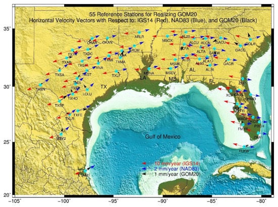
Figure 3.
Horizontal velocity vectors of 55 reference stations with respect to International GNSS Reference Frame 2014 (IGS14) (red), North American Datum 1983 (NAD83) (blue), and GOM20 (black). Detailed information of all reference stations is listed in Appendix A Table A1.
We also conducted several tests by adding to or removing a few stations from the group of 55 reference stations. We found that the changes provided little to no impact on the final displacement time series of coastal GNSS stations. In theory, three common stations will be able to provide the seven parameters for reference frame transformation [31]. However, more reference stations improve the reliability of the reference frame transformations and provide higher confidence in assessing the stability of the reference frame [33]. The definition of frame stability will be addressed in the next session. To take advantage of the dense and long-history CORS infrastructure that is available within the GOM region, we use 55 reference stations to realize the regional reference frame. Note that the redundancy of reference stations does not add any burden to GOM20 users. Users do not need any reference stations in obtaining GOM20 coordinates, and they even do not need to worry about the future status of these reference stations.
The detailed information of these 55 stations is listed in Appendix A Table A1. The vast majority of reference stations span over 15 years. The average observational history is 13.5 years, with about 330 daily files (11 months) per year. The station with the shortest observational history is MSEV, with a history of 7.8 years as the end of 2019. MSEV is located in Ellisville, Mississippi. There are not so many qualified reference stations in the state of Mississippi compared to other nearby states. The three-component displacement time series of MSEV retain high linearity with little gaps. Therefore, MSEV is selected as a reference station for realizing GOM20.
3.2. Coordinate Transformation from IGS14 to GOM20
In the surveying and geodesy research community, the Helmert transformation method is used to transform Cartesian coordinates from a well-established global reference frame to a regional or local reference frame. There are two approaches for transforming the positional time series between two frames: a daily 7-parameter method and a total 7-parameter method [31]. The daily 7-parameter method is often used for transforming GNSS-derived positional coordinates between two reference frames day by day. For examples, UNAVCO employs the daily 7-parameter transformation method in producing daily solutions for the Plate Boundary Observatory (PBO) network [19]; the Nevada Geodetic Laboratory at the University of Nevada, Reno employs the daily 7-parameter transformation method in producing daily solutions with respect to the North American Reference Frame (NA12) [34]. However, calculating daily transformation parameters can be a burden for most practical users. During the past years, we have developed a total 7-parameter method for transforming Earth-Centered-Earth-Fixed (ECEF) Cartesian (XYZ) coordinate time series from a global reference frame to a regional reference frame. The details of the method are introduced in our recent publications for establishing regional reference frames in North China [35], Houston metropolitan region [36], and the Caribbean [33].
GOM20 is aligned in origin and scale with IGS14. The PPP solutions with respect to IGS14 are presented in an ECEF-XYZ coordinate system. The ECEF-XYZ coordinates with respect to GOM20 can be obtained by the following formula, Equation (1):
where , , and are the ECEF-XYZ coordinates (at epoch t) of a site with respect to IGS14; , , and are the ECEF-XYZ coordinates of the site with respect to GOM20. The units of these XYZ coordinates are meters. is the epoch that aligns the coordinates with respect to these two reference frames, which is fixed at epoch 2015.0 (year) for GOM20. A site retains identical XYZ coordinates with respect to IGS14 and GOM20 at epoch 2015.0. , , , , , and are constant parameters indicating the rates (one-time derivates) of translational shifts and rotations along the x, y, an z coordinate axes between two reference frames. These seven parameters: , , , , , , and , are listed in Table 1.

Table 1.
Seven Parameters for Realizing GOM20.
To study ground deformation at the Earth’s surface, firstly, the ECEF-XYZ coordinates are transformed to GOM20 from IGS14; secondly, the geocentric XYZ coordinates are converted to a geodetic orthogonal curvilinear coordinate system (longitude, latitude, and ellipsoid height) referencing to the GRS80 ellipsoid; thirdly, the longitude and latitude coordinates are projected to a two-dimensional local horizontal plane for tracking superficial ground deformation in the north-south (NS) and east-west (EW) directions at each site. The change of ellipsoid heights over time is used to measure the up-down (UD) movement (subsidence or uplift). In practice, the vertical displacements (subsidence or uplift) derived from the ellipsoid heights and orthometric heights are the same [37].
3.3. Stability of GOM20
There is no widely accepted definition for the stability or accuracy of reference frames. These two terms are often applied interchangeably. The basic rule is that a stable site should retain near-zero velocities over time in all three directions (NS, EW, and UD) with respect to the stable reference frame. The term accuracy emphasizes the difference between the real site velocities and the supposed zero velocities at stable sites, while the stability emphasizes the accumulation of the positional shift over time. The stability of a static reference frames degrades over time since a linear movement (over time) is assumed in realizing the stable frame transformation. Eventually, the positional error becomes too imprecise with respect to user expectations. The stability of a reference frame determines its ability to extrapolate station coordinates accurately into the past and the future beyond the frame range [34]. In practice, the stability or accuracy of a regional reference frame is often evaluated by the root-mean-square (RMS) of the velocities of all reference stations with respect to the reference frame [33]. In essence, the lifetime of a static reference frame depends on the rigidity of the crustal block that the network of reference stations covers. The reference station network of GOM20 indicates a relative horizontal RMS accuracy of 0.3 mm/year and a vertical RMS accuracy of 0.5 mm/year (see Appendix A Table A1), suggesting that the GOM region is rigid at a half-millimeter per year level. Nevertheless, users should exercise appropriate cautions in interpolating site velocities at a sub-millimeter per year level for long-term ground deformation studies.
According to our previous investigations, the RMS-accuracy (repeatability) of the PPP daily positions is approximately 2 to 4 mm in the horizontal directions and 6 to 8 mm in the vertical direction within the GOM region [32,38]. As mentioned earlier, the stability of GOM20 is at a level of 0.3 mm/year in the horizontal directions and 0.5 mm/year in the vertical direction. Thus, GOM20 could result in accumulated positional-errors of 4.5 mm in the horizontal directions and 7.5 mm in the vertical direction across a 15-year window, which are still comparable with the RMS-accuracy of the daily GNSS measurements (PPP solutions). GOM20 is aligned to IGS14 at 2015.0. Hence, the potential positional errors 15 years before and after epoch 2015.0 (2000–2030) are still within the accuracy of the daily GNSS measurements. Though GPS datasets as early as 1990 are available within the GOM region, only a few stations have data before 1995, and over 98% GNSS stations were installed after 2000 (see Figure 2). In general, the daily positions derived from GPS data in the 1990s retain a poorer positional accuracy than the daily positions since 2000 because of fewer available satellites and reference frame stations available in the 1990s [38,39]. Thus, the accumulated positional errors associated with GOM20 may still lie within the accuracy of daily GPS measurements, even for the data before 2000. Accordingly, GOM20 can be confidently used for a time window from the 1990s to 2030 without causing positional errors larger than the accuracy of daily GNSS measurements.
In order to verify the stability of GOM20, we checked the positional time series of two long-history (27 years: 1993–2019) GNSS antennas (ADKS and LKHU) in the greater Houston area. Figure 4 depicts the three-component (NS, EW, UD) positional time series of ADKS and LKHU with respect to GOM20. The positions are relative positions referred to the absolute positions at epoch 2015.0. It is worth noting again that a site retains identical absolute positions with respect to GOM20 and IGS14 at epoch 2015.0. The GNSS antenna of each station is mounted on the top of the inner pole of a deep borehole extensometer. ADKS is located at Addicks, a western suburb of Houston. The antenna pole of ADKS is anchored at the bottom of the Evangeline aquifer, approximately 549 m below the local land surface. LKHU is located at Lake Houston, a northern suburb of Houston. The antenna pole of LKHU is also anchored at the bottom of the Evangeline aquifer, approximately 591 m below the local land surface. Detailed information about the two GNSS stations is presented in our previous publications [40,41]. The Evangeline aquifer is the major aquifer providing groundwater for industry and public use in the greater Houston area [42,43]. According to our previous investigations, present sediment compactions at the two sites occurred within the top portion of the Evangeline aquifer and its overlay aquifer, Chicot aquifer [41]. There are no reported ongoing faulting activities adjacent to the two locations. Thus, the two sites should be stable in all three directions with respect to GOM20. The plots in Figure 4 indicate that there are no steady displacement trends at both sites over 27 years. That means both sites are stable over time with respect to GOM20. The 27-year displacement time series verify that GOM20 provides a reliable reference in assessing the long-term site stability within the GOM region.
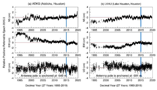
Figure 4.
Three-component positional time series at two long-history GNSS sites (ADKS, LKHU) in the greater Houston area. The relative positions are referred to the positions with respect to GOM20 at epoch 2015.0 (cyan line), which are the same as IGS14 positions at epoch 2015.0.
4. Applications of GOM20
GOM20 provides a coherent reference frame for aligning ground deformation within the GOM region over time and space. Figure 5 depicts horizontal and vertical velocity vectors (with respect to GOM20) derived from GNSS observations within the GOM region. To minimize the temporal variations of vertical site velocities, we only depict the velocity vectors at stations that span at least three years and have at least 1000 observational files within the period from 2010 to 2019. The velocities are calculated with the Median Interannual Difference Adjusted for Skewness (MIDAS) method [44]. MIDAS breaks displacement time series into 1-year-long (365 days) segments and selects the median slope of the selected segments as the slope (trend) of the whole time series. We compared the site velocities calculated by MIDAS and the conventional least-squares method. It is found that the site velocities (trends) obtained by the two methods agree well in general and the MIDAS method does a better job in minimizing the effects of outliers, step discontinuities, and seasonal movements superimposed into GNSS time series.
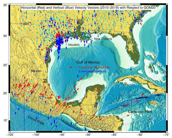
Figure 5.
GNSS-derived horizontal (red) and vertical (blue) velocity vectors at stations with a history over three years and total observational days over 1000 within the period from 2010 to 2019. The arrows of the subsidence vectors at several sites in central Mexico go beyond the map because of the great values.
MIDAS computes a velocity uncertainty that is based on the distribution of sampled slopes of 1-year-long displacement time series. For the 500 stations shown in Figure 5, the velocity uncertainty varies from ±0.2 to ±0.6 mm/year in the horizontal directions and ±0.3 to ±1.0 mm/year in the vertical direction. The MIDAS velocity uncertainty approximates to one standard deviation of the selected slopes, which indicates a 68% confidence interval (CI) of the velocity estimate. The uncertainty is inversely correlated with the time span of GNSS datasets. A longer observational history and fewer data gaps often result in a smaller uncertainty of the velocity estimate. In general, the uncertainty is resulted by noises superimposed into the GNSS-derived displacement time series. The noise sources are dominated by seasonal ground deformation due to changes in groundwater levels and atmospheric loading, monument instability (random walk noise), and errors in satellite orbits and GNSS equipment (receivers, antennas). The noises can be best described by a combination of white noise and flicker noise [45].
The velocity vectors illustrated in Figure 5 indicate that the GOM region is overall stable except the southwest region, which is affected by the subducting of the Rivera and Cocos Plates beneath the North American Plate along the Middle America subduction zone (Figure 1). Rivera and Cocos Plates are relatively young (10–25 Ma) oceanic plates; both plates are subducting along the Middle American Trench at different convergence rates [46]. The GNSS-derived velocity vectors along the western coast of Central Mexico vividly indicate that the convergence rate increases progressively to the southeast along the Middle American Trench. Driven by the subduction of the Cocos Plate, the western coast of Central Mexico retains steady movements towards the northeast (1 to 3 cm/year) and downward (0.5 to 1 cm/year). The maximum horizontal movement (OXPE: 2009–2019, 2.8 cm/year) is recorded at the town of Puerto Escondido on the Oaxacan coast. This site also retains steady subsidence of 7.3 mm/year.
4.1. Urban Subsidence
Among these 1000 continuous GNSS stations plotted in Figure 1, seven stations recorded subsidence rates over 2 cm/year, which are located in major cities of central Mexico (Figure 6). Over twenty stations in the greater Houston area recorded subsidence rates between 1 cm/year and 2 cm/year. GNSS-derived land subsidence and faulting activities in the greater Houston area have been investigated by Harris-Galveston Subsidence District [47], US Geological Survey [43], and the University of Houston [39,48,49]. Therefore, this study will not explore the details of subsidence and faulting activities within the greater Houston area.
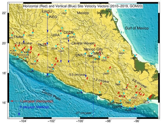
Figure 6.
Map showing GNSS-derived horizontal (red) and vertical (blue) velocity vectors at long-term stations in central Mexico. The distance between UAGU and INEG is 6.5 km. The arrow of the subsidence vector at MMX1 goes beyond the map because of the great value (27 cm/year).
These seven GNSS stations experienced rapid subsidence (>2 cm/year) are MMX1 (subsidence rate: 27.1 cm/year), INEG (subsidence rate: 4.0 cm/year), UAGU (subsidence rate: 7.0 cm/year), CECM (subsidence rate: 6.3 cm/year), UNTO (subsidence rate: 5.5 cm/year), UIRA (subsidence rate: 6.7 cm/year), and TNZA (subsidence rate: 7.5 cm/year). They are located in urban areas that rely mainly on groundwater to sustain agriculture, industrial, and domestic water needs [50]. The GPS-derived subsidence time series of these stations are depicted in Figure 7. MMX1 is located at the International Airport of Mexico City, Mexico, which recorded steady subsidence of 26.7 cm/year during the period from 2010 to 2016. The subsidence accelerated to approximately 31 cm/year during 2017 and 2018 (Figure 7a). The subsidence time series in 2019 shows a trend of slowing down. To our knowledge, the overall subsidence rate of 27.1 cm/year is the most rapid subsidence that is ever recorded by continuous GNSS in urban areas.
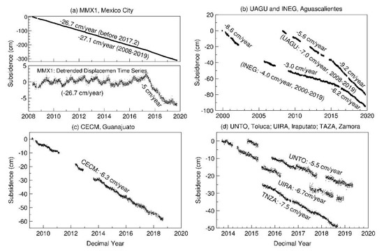
Figure 7.
Subsidence time series at seven GNSS stations that recorded rapid subsidence (>2 cm/year) in central Mexico (see Figure 6). (a) MMX1 in Mexico City; (b) UAGU and INEG in Aguascalientes; (c) CECM in Guanajuato; (d) UNTO in Toluca, UIRA in Iraputato, and TAZA in Zamora.
UAGU and INEG are two GNSS stations located at the northern and southern Aguascalientes, the capital of the Mexico state Aguascalientes, 430 km northwest of Mexico City. Aguascalientes is situated over a vast unconfined aquifer system encompassing three Mexico states. The growing population and increased agricultural and industrial activities have resulted in intensive groundwater extraction since the 1970s [51]. The distance between UAGU and INEG is 7.6 km (Figure 6). The subsidence rate at INEG was 8.6 cm/year in the early 2000s, which slowed down to 3.0 cm/year during the late 2000s and early 2010s (2005–2014); however, subsidence at this site accelerated since 2015 and retains an ongoing average subsidence rate of 6.2 cm/year (2015–2019) (Figure 7b). UAGU recorded steady subsidence of 5.6 cm/year during the late 2000s and early 2010s (2008–2014). Subsidence at this site also accelerated since 2015 and retains an ongoing subsidence rate of 9.2 cm/year (2015–2019) (Figure 7b). The subsidence time series at UAGU and INEG depict extraordinary temporal and spatial variations of urban subsidence, which have also been observed in many other sinking cities [2,32,39]. In general, rapid subsidence in urban areas is primarily caused by groundwater pumping; the rate of subsidence varies over time and space in response to the variations of pumping amount, groundwater levels, and geologic and hydrologic conditions of local aquifers.
CECM recorded steady subsidence with a rate of 6.3 cm/year (2009–2019) (Figure 7c). CECM is located in Celaya, a city in the state of Guanajuato, Mexico. UNTO recorded steady subsidence with a rate of 5.5 cm/year (2014–2019) (Figure 7d). UNTO is located in Toluca, the state capital of the State of Mexico. Toluca is the fifth largest city in Mexico. UIRA recorded steady subsidence with a rate of 6.7 cm/year (2013–2019) (Figure 7d), which is located in Irapuato, a Mexican town in the central region of the state of Guanajuato, approximately 300 km northwest of Mexico City. TNZA recorded steady subsidence of 7.5 cm/year (2015–2019) (Figure 7d). TNZA is located in Zamora, a city in western Mexico state of Michoacán.
Land subsidence in major cities in central Mexico has been frequently investigated using InSAR techniques [50,52,53]. Since InSAR employs the difference in the carrier signal phase between Synthetic Aperture Radar (SAR) images to recover relative displacements over space, there is a benefit to tying InSAR-derived displacements to absolute positions with respect to GOM20, which is aligned to the global reference frame IGS14 at epoch 2015.0. The GNSS-derived positional time series with respect to GOM20 will provide ground-truth to calibrate and constrain InSAR-derived subsidence measurements over time and space [54].
4.2. Coastal Subsidence and Faulting
Subsidence has been widely recognized as a driver of geomorphic change in the northern Gulf of Mexico [2,55,56]. However, there is considerable disagreement over the subsidence rates and the interpreted temporal and spatial variability in these rates. The vertical velocity vectors depicted in Figure 5 indicate that vertical land deformation rates along the Florida portion of the GOM coast are within ±1 mm/year with respect to GOM20. Figure 8 depicts GNSS stations within an 800-km-long low-elevation belt along the coast of eastern Texas, Louisiana, Mississippi, and Alabama. There are two long-history GNSS stations on the coastal line of Alabama: ALD1 and MOB5. The antenna of ALD1 is mounted on a building on the Dauphin Island, a barrier island at the Gulf of Mexico, and has an observational history of 11 years (2009–2019). MOB5 is located at Fort Morgan at the mouth of Mobile Bay, Alabama, and has an observational history of approximately 18 years (1995–2012). The distance between ALD1 and MOB5 is about 6 km. Both stations recorded steady subsidence of 2.0 ± 0.7 mm/year. The near-coast GNSS station ALFO (2010–2019) in Foley, Alabama, also recorded steady subsidence of approximately 2.0 ± 0.7 mm/year. There are two long-history GNSS stations along the Mississippi coast: MSGA (2008–2019) and MSIN (2010–2019). MSGA recorded a near-zero vertical velocity (~0.1 mm/year). MSIN recorded steady subsidence of 2.2 ± 0.8 mm/year. Long-history observations at these stations suggest that the ongoing subsidence along the coastal lines of Alabama and Mississippi is at a level of 2 mm/year.
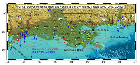
Figure 8.
Map showing GNSS-derived subsidence along the coast of eastern Texas, Louisiana, Mississippi, and Alabama. The red lines represent fault lines (data from AAPG [57]).
Figure 8 indicates that the Louisiana coast experiences subsidence from 3 to 6.5 mm/year. The maximum subsidence rates were recorded by two GNSS stations on the coastline of the Mississippi River delta: LMCN (2003–2019, subsidence rate: 6.3 ± 0.6 mm/year) and GRIS (2005–2019, subsidence rate: 6.5 ± 0.5 mm/year). There is a clear trend that the subsidence rate generally decreases westward, eastward, and landward with respect to the Mississippi River delta. From the inland to the front of the delta, subsidence rate increases from 2 to 4 mm/year (MGW3: 2.0 ± 1.2 mm/year; AME4: 2.8 ± 1.1 mm/year; LAGM: 3.1 ± 0.8 mm/year; HOUM: 3.8 ± 0.6 mm/year; BVHS: 3.9 ± 0.6 mm/year) to 6.5 mm/year (LMCN: 6.3 ± 0.6 mm/year; GRIS: 6.5 ± 0.5 mm/year). Figure 9 illustrates the subsidence time series of these seven coastal GNSS stations on the Mississippi River delta. Overall, these seven sites retain steady subsidence over time, which are remarkably different from urban subsidence dominated by groundwater withdrawal, as shown in Figure 7b. Modern subsidence in the Louisiana coastal area has been described as a result of (1) fluid withdrawal (groundwater, oil and gas) (up to a few centimeters per year) [2], (2) deep-seated tectonic movements (fault processes, up to a few millimeters per year) [6], (3) Holocene sediment compaction (up to a few millimeters per year) [58,59], (4) sediment loading (below 0.5 mm/year) [60,61,62], (5) glacial isostatic adjustment (below 1 mm/year) [63], and (6) surface water drainage and management [64]. It is worth pointing out that these processes are not fully independent from one another.
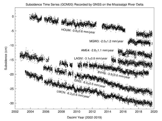
Figure 9.
The subsidence time series (with respect to GOM20) at seven GNSS stations within the Mississippi River Delta area. Locations of these seven GNSS stations are shown in Figure 8.
Dakka et al. [6] suggested that the steady subsidence in the Mississippi River delta area is likely due to deep-seated faulting. They proposed that the Mississippi delta area is located on the hanging wall of a large listric normal fault system. Figure 8 indicates that several GNSS stations in the delta area recorded steady horizontal movements (1 to 2 mm/year) toward the GOM, such as LMCN (EW: 1.2 ± 0.2 mm/year; NS: −0.6 ± 0.2 mm/year), AME4 (EW: −1.3 ± 0.5 mm/year; NS: −0.7 ± 0.5 mm/year), and FSHS (EW: 0.4 ± 0.3 mm/year; NS: −2.3 ± 0.2 mm/year). However, no coherent oceanward movement was observed within the Mississippi River delta area. The horizontal movement at FSHS is particularly significant, though there is not a reported fault line across this site. FSHS (2010–2019) recorded a steady horizontal movement toward the south with a velocity of 2.3 ± 0.3 mm/year and a steady downward movement (subsidence) of 1.7 ± 0.8 mm/year (Figure 10). FSHS is located at the southern part of Franklin, a small town in St. Mary Parish, Southern Louisiana. LAFR, another permanent GNSS station located in the same town, recorded similar velocities in all three directions. The distance between these two stations is approximately 2 km. Based on our experience with urban faults in Houston [9], the highly coherent and steady horizontal movements observed at the two sites are likely associated with local faulting activities.
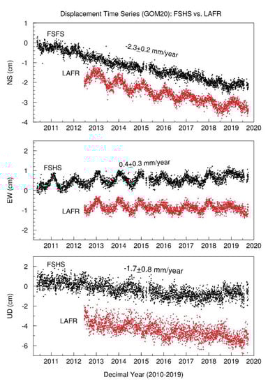
Figure 10.
Three-component displacement time series recorded by two closely-spaced (2 km) GNSS stations (FSHS and LAFR) in Franklin, southern Louisiana.
4.3. Delineating the Absolute Sea-level Rise Rate along the GOM Coast
Global sea level has been rising over the past century, and the rising rate has increased in recent decades due to global warming [65]. Sea level plays a critical role in wetland loss, coastal flooding, shoreline erosion, and flooding hazards from storms. In the long term, rising sea level also creates stress on groundwater systems and coastal ecosystems. As the sea-level rises, saltwater intrudes into freshwater aquifers, many of which sustain coastal ecosystems and provide water for municipal and agriculture. The Louisiana and Texas coastal areas are currently experiencing subsidence varying from 4 to 6.5 mm/year, as depicted in Figure 8.
Sea level is primarily measured using tide gauge stations along the coasts and satellite laser altimeters in the open ocean. The Center for Operational Oceanographic Products and Services (COOPS) at the National Ocean Service, National Oceanic and Atmospheric Administration (NOAA) of the US operates 25 long-history (>30 years) tide gauge stations along the GOM coast (Figure 11), which are a part of the National Water Level Observation Network (NWLON). The network operates 210 long-term, continuously operating water level stations throughout the US and its territories. NOAA/COOPS also provides routinely-updated analyses of the long-term trends and variability from tide gauge stations operated by international agencies. There are four long-history (>30 years) tide gauge stations on the Mexico portion of the GOM coast and one tide gauge station on the coast of Cabo San Antonio, Cuba. In total, there are 30 long-history tide gauge stations along the GOM coast (Figure 11). Long-term tide gauge records used for this study are downloaded from the NOAA COOPS (https://tidesandcurrents.noaa.gov/sltrends/sltrends.html). These measurements are monthly averages, which removes the effect of higher frequency phenomena to compute an accurate linear sea-level trend.
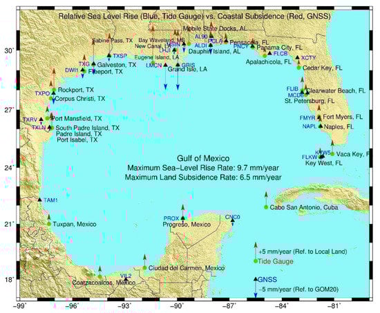
Figure 11.
Map depicting the relative sea-level (RSL) trends and vertical land movement trends derived from closely-spaced tide gauge and GNSS pairs. The RSL trends are referred to adjacent benchmarks fixed on land surface; the land movement trends are referred to GOM20.
Instead of measuring absolute (eustatic) sea-level changes, long-term tide gauge measurements provide information on relative sea-level changes. This is because tide gauges measure sea levels relative to reference benchmarks fixed on the local land surface through repeat leveling surveys. Therefore, the readings of tide gauges are a combination of the absolute sea-level changes and the local land vertical movements. Absolute sea-level rise is mostly due to a combination of thermal expansion of seawater and meltwater from glaciers and ice sheets. A smaller contributor to global sea-level rise could be the decline of aquifer storage capacity as a result of excessive groundwater pumping. The pumping-compaction process squeezes water out from aquifers and leads to permanent compaction of aquifers, eventually, moving water from inland to the sea.
The absolute global sea-level rise rate is critically important for evaluating the long-term risk of coastal flooding, erosion, and wetland loss at a regional scale. The stable regional reference frame and the long-history GNSS observations in the GOM region provide a fundamental infrastructure for delineating secular sea-level trends. In this section, we use closely-spaced GNSS and tide gauge measurements on Grand Isle, Louisiana (Figure 12), to describe the process of delineating absolute sea-level trends.
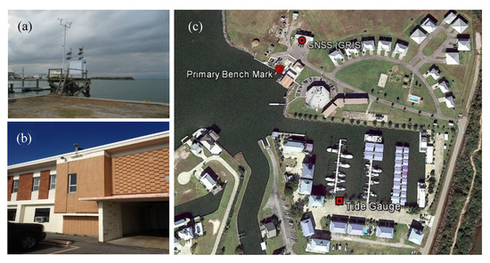
Figure 12.
Closely-spaced tide gauge and GNSS station (GRIS) at Grand Isle, Louisiana. (a) Grand Isle tide gauge station. The photo is obtained from National Ocean Service, NOAA (https://tidesandcurrents.noaa.gov/stationphotos.html?id=8761724). (b) The GNSS station GRIS. The site photo is obtained from NGS, NOAA (https://www.ngs.noaa.gov/CORS). (c) Google Earth image showing the locations of the tide gauge, GNSS (GRIS), and the primary benchmark fixed on a concrete sea wall for leveling tide gauge measurements.
Grand Isle is a barrier island at the southern edge of Barataria Bay, one of the large inter-distributary bays in the Mississippi River delta. The Grand Isle tide gauge sits atop of the barrier island, closely-spaced (250 m) with a long-term GNSS station GRIS (Figure 12a,b). The Grand Isle tide gauge was installed in 1947 and has been continuously operated for 73 years. The primary benchmark used for leveling the tide gauge measurements is a disk set on the top of a concrete sea wall adjacent to the tide gauge (https://tidesandcurrents.noaa.gov/benchmarks/8761724.html). There are a dozen of other benchmarks around the primary benchmark for assessing the long-term vertical movements of the primary benchmark. Thus, sea-level changes over time are tracked relative to a fixed station datum maintained by the benchmark network. The distance between the tide gauge and the primary benchmark is approximately 220 m; the distance between the tide gauge and the GNSS station is approximately 250 m (Figure 12c). GRIS is operated by the Center for Geoinformatics at Louisiana State University and has accumulated 15 years (2005–2019) of continuous GNSS observations (Figure 13). The antenna of GRIS is mounted on a two-floor concrete-brick building, 60 meters away from the primary benchmark on the concrete sea wall. Since the GNSS antenna is only 250 m away from the tide gauge site, the 15-year GNSS observations would be able to provide accurate vertical land movement trend at the tide gauge site.
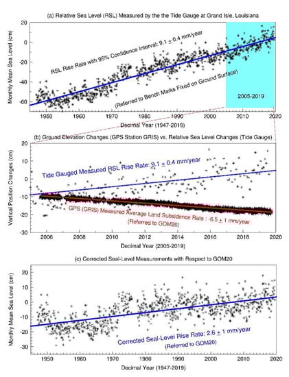
Figure 13.
Plots illustrating the process of recovering absolute sea-level rise trend. (a) The monthly mean sea level measurements recorded by the tie gauge (Figure 12a). The sea level values are relative to the most recent Mean Sea Level datum established by COOPS. (b) A comparison of vertical land movements measured by GPS (Figure 12b) and sea-level changes measured by the tide gauge (2005–2019). The sea-level changes are referred to the primary benchmark fixed on the adjacent concrete sea wall (Figure 12c). (c) The absolute sea-level rise trend with respect to GOM20. The uncertainties of the seal-level-rise rate and the land subsidence rate approximately indicate the 95% confidence interval.
Recent studies conducted by the research group at the Tulane University suggest that a significant portion of subsidence in the Mississippi River delta area occurs within the shallow portion (top 5 m) of the sediments [66,67,68]. The foundations of buildings in the soft delta area are often deeper than similar structures inland. The monuments of the tide gauges could be considerably deep in order to sustain the long-term stability of the gauges. The deeply buried foundations may exclude certain compaction of shallow sediments [69]. If the depths of the foundation of the building that GNSS is mounted on and the foundation of the tide gauge are considerably different, the GNSS antenna and tide gauge may experience different subsidence, and both could be different from the subsidence at the land surface (total compaction). Thus, the absolute sea-level changes derived from the method illustrated in Figure 13 could be biased. A further investigation of this issue will be conducted in our future study.
Figure 13a depicts the 73-year (1947–2019) monthly mean sea-level (MSL) measurements recorded by the tide gauge at Grand Isle, Louisiana. The MSL values are referred to the most recent Mean Sea Level Datum established by COOPS. The relative sea-level rise rate is 9.1 mm/year with a 95% CI of ±0.4 mm/year. That means the site has submerged to water approximately 65 cm during the past 73 years. The process for calculating the 95% CI is documented in the NOAA Technical Report [70]. Figure 13b depicts the land subsidence time-series recorded by the GNSS station GRIS and the relative sea-level rise recorded by the tide gauge during 15 years from 2005 to 2019. The land subsidence rate is 6.5 mm/year with a 95% CI of ±1 mm/year with respect to GOM20. The 95% CI is estimated by twice the velocity uncertainty obtained according to the MIDAS method [44]. Assuming the local land retained the same subsidence rate during the history of the tide gauge, the absolute sea-level trend at the tide gauge site can be obtained by subtracting out the land subsidence rate (6.5 mm/year) from the relative sea-level rise rate (9.1 mm/year). The reasonableness of the assumption will be discussed later. Figure 13c depicts the absolute sea-level rise time series with respect to GOM20. The absolute sea-level rise rate at the tide gauge site is 2.6 mm/year (with respect to GOM20). The uncertainty (95% CI) of the corrected sea-level rise rate could be approximated by the larger one between the uncertainty of the sea-level rise rate (± 0.4 mm/year) and the uncertainty of the land subsidence rate (± 1 mm/year).
The relative sea-level rise rates at 30 tide gauge stations along the GOM coast are depicted in Figure 11. The rate ranges from 2.1 mm/year (106 years: 1914–2019) at Cedar Key, Florida, to 9.7 mm/year (36 years: 1939–1974) at Eugene Island, Louisiana. Ten tide gauge stations along the Florida coast recorded relative sea-level rise rates varying between 2 to 4 mm/year. Two tide gauge stations along the Alabama coast recorded relative sea-level rise rates approximate to 4 mm/year. One tide gauge station at the Mississippi coast recorded relative sea-level rise rate of 4.6 mm/year. There are three long-history tide gauges along the coast of Louisiana. Two stations located at the frontier of the Mississippi River delta recorded significant relative sea-level rise rates: Eugene Island: 9.7 mm/year (36 years: 1939–1974) and Grand Isle: 9.1 mm/year (73 years: 1947–2019). One station located at the back of the Mississippi River delta recorded a slower sea-level rise rate: 5.4 mm/year (New Canal, 38 years: 1982–2019). There are nine long-history tide gauge stations along the coast of Texas. Five stations north of Corpus Christi recorded relative sea-level rise rates from 5 to 7 mm/year. The other four Texas stations south of Corpus Christi, as well as four gauges along the Mexico coast and one station at the coast of Cuba, recorded sea-level rise rates at 2 to 3 mm/year.
Since all tide gauges along the GOM coasts are within the same oceanic basin, the absolute sea-level change rates at different sites should be approximately the same. Thus, the variations in relative sea-level rise rates seen here (Figure 11) primarily reflect differences of local land movements (subsidence or uplift). We selected a closely-spaced GNSS station to estimate the land vertical movement trend at each tide gauge site. The selection of GNSS stations is based on a combining consideration of the distance to the tide gauge, the observation history of the GNSS, and local tectonic movements. The selected GNSS stations for 30 tide gauge stations are depicted in Figure 11. Twenty-nine long-history GNSS stations are chosen to match these 30 tide gauge stations. Two tide gauge stations at Coatzacoalcos and Ciudad del Carmen, Mexico, share the same GNSS station (VIL2: 2003–2019). The average observational history of these 29 GNSS stations is 11 years. The detailed information of these 30 pairs of closely-spaced tide gauge and GNSS stations are listed in Table 2. The observational history of these GNSS stations varies from 3 years (FLIB: 2017–2019) to 19 years (MCD5: 2001–2019).
Table 2.
Closely-spaced Tide Gauge and GNSS stations along the GOM coast.
Since there are numerous GNSS stations along the US portion of the GOM coast, a long-history GNSS station can often be found for a tide gauge station within a few kilometers. The shortest distance between a tide gauge and its corresponding GNSS is within one kilometer, such as the distance (260 m) between the tide gauge at Grand Isle, LA (1947–2018) and GNSS station GRIS (2005–2019), and the distance (300 m) between the tide gauge on Dauphin Island, Alabama (1966–2019) and the GNSS station ALDI (2009–2019). Unfortunately, there are few long-history GNSS stations along the Mexico and Cuba portions of the GOM coast. The distance between the tide gauge at Cabo San Antonio, Cuba (1971–2016) and its corresponding GNSS station CNC0 (2007–2019) is up to 214 km. CNC0 is a COCONET station located in Cancun, Mexico. CNC0 recorded steady subsidence of 1.4 mm/year (2007–2019). Another GNSS station (UNPM), located in Puerto Morelos, 35 km south of Cancun, Mexico, also recorded steady subsidence of 1.4 mm/year. Three selected GNSS stations (TAMI: 2009–2019, VIL2: 2003–2019, and PROX: 2011–2015) for estimating the vertical land movement at four tide gauge sites along the Mexico coast also recorded subsidence rates of approximately 1.5 mm/year (with respect to GOM20). There is no considerable vertical crust deformation within the southern GOM region and there is no massive groundwater and oil gas extractions along the southern coast of GOM. Thus, the vertical ground movement trends derived from these four GNSS stations provide reliable estimates of the long-term vertical land movements at their corresponding tide gauge sites.
Figure 14 depicts sea-level rise rates at 30 tide gauge sites with respect to GOM20, which are obtained according to the method illustrated in Figure 13. The average absolute sea-level rise rate with respect to GOM20 is 2.6 mm/year, with a standard deviation of approximate 0.5 mm/year (1), which suggests a 95% spatial confidence interval of ±1 mm/year (2). Figure 13c suggests that the temporal uncertainty (95% CI) of the absolute sea-level rise trend is also at a level of approximately ±1 mm/year. The tide gauge at Sabine Pass, Texas, exhibits the most substantial absolute sea-level rise rate (−4.86 mm/year). Sabine pass is the state boundary between Texas and Louisiana. This site is located at the Texas side of the Sabine Pass, approximately 6.4 km inland from the coastal line. Sabine pass is the connection of the Sabine Lake and GOM. The regional ocean currents at the tide gauge site may be slightly different from tide gauge stations on the coastal line. The GNSS station (TXSP) used to estimate the local land movement at Sabine Pass also had a short history of only four years (2016–2019). Accordingly, we exclude the absolute sea-level rise rates at the Sabine Pass site as an outlier in calculating the average sea-level rise rate and its corresponding standard deviation. The high sea-level rise rate (3.6 mm/year) recorded at New Canal, a shipping canal in New Orleans, Louisiana, could also be biased by regional ocean currents.
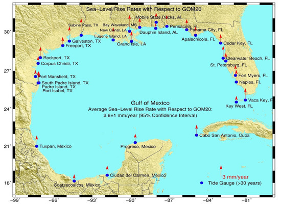
Figure 14.
Absolute several-level rise rates (with respect to GOM20) at 30 tide gauge stations along the coastline of GOM.
The method for delineating an absolute sea-level trend assumes that both relative sea-level and vertical land movements retain linear trends over time. Nevertheless, the assumption may be valid only in a limited time window. These 30 tide gauge stations have an average history of 56 years, while their corresponding GNSS stations have a much shorter history, approximately one decade. Among these 29 GNSS stations, twenty-one stations (72%) recorded vertical movement trends within ±2 mm/year; six stations (20%) recorded downward land movement trends between 2 to 3 mm/year; only two stations at the Mississippi delta coast recorded downward movement trends of approximately 6.5 mm/year (GRIS: 6.5 mm/year; LMCN: 6.4 mm/year). From the view of plate tectonics, the eastern (Florida), western (western Texas, Mexico), and southern (Mexico, Guba) portions of the GOM coast are stable over time, as demonstrated in Figure 5. Accordingly, it is reasonable to extend the GNSS derived land movement trends to the observational history of tide gauges. Since these 30 tide gauges have an average history of approximately a half-century, we suggest that the interpolation of 2.6 ± 1 mm/year (95% CI) sea-level rise rate with respect to GOM20 be limited to the past five decades (the 1970s—2010s).
The 2.6 ± 1 mm/year sea-level rise rate with respect to GOM20 can be regarded as a regional adjustment to the global mean sea-level rise (GMSLR). In general, the estimates of GMSLR during the 20th-century range from 1.6 to 3.0 mm/year [71,72,73,74,75,76]. These studies also emphasized temporal variations of the tide-gauge-derived GMSLR. Holgate [71] reported global sea-level rise rates of 2.03 ± 0.35 mm/year (1904–1953), 1.45 ± 0.34 mm/year (1954–2003), and 1.74 ± 0.16 mm/year (1900–2000). Church and White [74] reported GMSLR of 1.7 ± 0.2 mm/year (1990–2009) and 1.9 ± 0.4 mm/year (1961–2009). Hay et al. [76] reported GMSLR of 1.2 ± 0.2 mm/year (1902–1990, 90% CI) and 3.0 ± 0.7 mm/year (1993–2010). It appears that the 2.6 ± 1 mm/year seal-level rise rate along the GOM coast is slightly higher than the recently reported GMSLR. The 2.6 ± 1 mm/year is also slightly higher than recently reported average absolute sea-level rise rate along the GOM coast. Letetrel et al. [77] reported an absolute sea-level rise rate of 2.0 ± 0.4 mm/year based on long-history observations from five closely-spaced tide gauge and GNSS pairs and satellite altimetry data along the GOM coast.
5. Discussion
5.1. GOM20 Versus NAVD88
The US National Spatial Reference System (NSRS) is currently realized by the North American Datum of 1983 (NAD83) and the North American Vertical Datum of 1988 (NAVD88). NAD83 and NAVD88 are the official horizontal and vertical datums for coastal mapping and subsidence studies in the conterminous United States (CONUS). However, both NAD83 and NAVD88 rely on physical survey marks on land that deteriorate over time. To improve NSRS, NGS will replace NAD83 and NAVD88 with the North American Terrestrial Reference Frame of 2022 (NATRF2022) and the North American-Pacific Geopotential Datum of 2022 (NAPGD2022) in 2022 (https://geodesy.noaa.gov). NAVD88 was established in 1991 by the minimum-constraint adjustment of geodetic leveling observations in North American continental covering Canada, the United States, and Mexico. In the adjustment, only the height of the primary tidal benchmark at Father Point, Rimouski, Quebec, Canada, was held fixed. The Father Point is approximately 2500 km away to the north coast of GOM. The definition of NAVD88 uses the Helmert orthometric height, which can be obtained by the geoid height at the site plus the ellipsoid height derived from GNSS observations [37]. Currently, the geoid height with respect to the NAD83 ellipsoid can be estimated by the most recent geoid model GEOID18 (https://www.ngs.noaa.gov/GEOID/GEOID18/). In practice, the geoid height at a site is regarded as a constant number over time. Thus, a trend of the orthometric height time series (with respect to NAVD88) is the same as the trend of the ellipsoidal height time series (with respect to NAD83) [37].
Figure 15a depicts the three-component displacement time series at GNSS station GRIS with respect to NAD83 and GOM20. To get the NAD83 coordinate time series, firstly, the IGS14 coordinates are transformed to IGS08 coordinates according to the method provided by IGS [12], and the IGS08 coordinates are transformed to NAD83 coordinates according to the method provided by NGS [78]. The displacement time series with respect to NAD83 indicate a movement toward the east direction with a steady velocity of 1.4 mm/year and a downward movement (subsidence) of 8.3 mm/year. The subsidence rate with respect to NAD83 is approximately 2 mm/year faster than the subsidence rate with respect to GOM20 (6.5 mm/year). GRIS is closely-spaced (250 m) with the tide gauge located on the Grand Isle, Louisiana (Figure 12). Figure 14 suggests that the absolute sea-level rise rate at the Grand Isle, Louisiana tide gauge site is 2.6 mm/year if GOM20 is used as a reference frame. However, the absolute sea-level rise rate would be reduced to 0.8 mm/year if NAD83 (or NAVD88) is used as a reference frame. The difference of 2 mm/year is remarkable for sea-level studies. It is not a simple question as to which value is right or wrong because they specifically refer to different reference frames. A significant difference between NAVD88 and GOM20 is that GOM20 used references (points) adjacent to the Gulf coast (within 500 km to the coastal line), while NAVD88 used references are much further away from the Gulf coast.
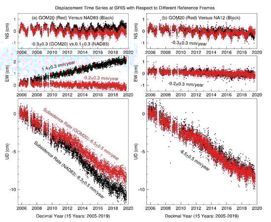
Figure 15.
Three-component displacement time series at GNSS station GRIS with respect to (a) GOM20 versus NAD83, and (b) with respect to GOM20 versus NA12. GRIS is located on the barrier island, Grand Isle, Louisiana (see Figure 12).
Nevertheless, the references closer to the Gulf coast will share more common ground movements with the GOM coastal area than those references far away from the coast. Glacial isostatic adjustment (GIA) is a typical common vertical movement that can be entirely removed by the regional reference frame. As to the vertical land movements due to GIA, they are spatially uniform within the GOM region and have amplitudes less than 1 mm/year [79]. Certainly, using references adjacent to the coastal area would make more sense to appraise the long-term risks associated with coastal subsidence, sea-level rise, flooding, and erosion.
5.2. GOM20 Versus NA12
NA12 is another continental-scale reference frame that has also been applied for geological hazards and crustal motion studies in North American [34]. NA12 is designed to have no-net-rotation (NNR) with respect to the stable interior of the North American Plate. Figure 15b illustrates the three-component displacement time series at GNSS station GRIS with respect to GOM20 and NA12. The time series with respect to NA12 is obtained from the Nevada Geodetic Laboratory (http://geodesy.unr.edu). No outliers have been removed. The comparison indicates that the long-term ground deformation trends with respect to both reference frames are almost identical.
Nine of the 30 core reference stations used for realizing NA12 are also used as reference stations for realizing GOM20. They are BKVL (2003–2019), GNVL (2002–2019), OKAN (2002–2019), ORMD (2003–2019), PBCH (2005–2019), TXLL (2005–2019), TXSN (2005–2019), XCTY (2004–2019), and ZEFR (2003–2019) (Appendix A Table A1). One of the major differences between NA12 and GOM20 is that NA12 employs the daily 7-parameter transformation method for transforming EEF-XYZ coordinates from the global reference frame (IGS14) to the regional reference frame (NA12). In contrast, GOM20 employs the total 7-parameter transformation method for transforming EEF-XYZ coordinates from the global reference frame (IGS14) to the regional reference frame (GOM20). NA12 users need daily 7-parameters provided by the Nevada Geodesy Laboratory to convert IGS14 coordinates to NA12. In contrast, GOM20 users only need the seven parameters listed in Table 1 to convert the whole time series from IGS14 to GOM20. Furthermore, the 7-parameters used by GOM20 are unattached to the future status of these reference stations. That is to say, GOM20 provides more convenient and reliable access to users than NA12.
5.3. Broad Applications of GOM20
GOM20 provides a consistent platform to integrate positional observations over space and time from different remote sensing techniques to a unified geodetic reference and enables multidisciplinary and cross-disciplinary research. The long-term GNSS observations within the GOM region have accumulated valuable datasets for the research community. Hydrologists may use these datasets for studying ground deformation resulting from fluid withdrawal, aquifer compaction, and seasonal hydrologic and atmospheric pressure loading; geomorphologists may use these datasets for studying long-term coastal erosion and wetland loss problems along the GOM coast; oceanographic and sea-level researchers may use these datasets for calibrating long-term sea-level changes along the GOM coast; researchers in the field of remote sensing may use GNSS-derived displacement time series as “ground truth” for calibrating or validating subsidence estimations from remote sensing techniques, such as InSAR, airborne LiDAR, and UAV-photogrammetry. The long-term GNSS measurements also provide first-hand ground truth datasets for local governments to assess risks from coastal subsidence and sea-level rise and make plans for future coastal development. Hopefully, this study will further stimulate coastal hazards investigating and land-use planning discussions along the GOM coast.
GOM20 also enables an approach of using stand-alone GNSS to conduct accurate ground deformation monitoring, as well as structural health monitoring, such as the long-term stability monitoring of offshore platforms within GOM. By transforming PPP solutions to a regional reference frame, users do not need to install any ground reference stations in the field and do not need to include any reference data in their data processing. The stand-alone GNSS surveying method will substantially reduce field logistics costs and, therefore, will revolutionize the way for conducting geological hazards (landslides, subsidence, faulting) and structural health monitoring in the GOM region.
6. Conclusions
Current geodetic infrastructure within the GOM region makes it possible to precisely track long-term (e.g., > 3 years) ground deformation at the level of 0.5 mm/year and above using stand-alone GNSS observations. This study summarized the current GNSS stations along the GOM coast and established a stable regional reference frame. The primary product from this study is the seven parameters (Table 1) for converting the ECEF-XYZ coordinate time series from the global reference frame IGS14 to the regional reference frame GOM20. The frame stability of GOM20 is approximately 0.3 mm/year in the horizontal directions and 0.5 mm/year in the vertical direction. GOM20 can be confidently used from the 1990s to 2030 without causing positional errors larger than the precision of daily-PPP solutions. It’s certainly important to be cautious when interpreting site velocities at a level of submillimeter per year.
GOM20 will be incrementally improved and synchronized with future updates of IGS reference frames. According to this study, subsidence faster than 2 cm/year is ongoing in several major cities in central Mexico, and the most rapid urban subsidence is approximately 27 cm/year in Mexico City; a large portion of the Texas and Louisiana coasts is subsiding at 3 to 6.5 mm/year, and the most rapid coastal subsidence is up to 6.5 mm/year at the coastline of Mississippi River delta; the present average sea-level rise rate along the GOM coast is 2.6 ± 1mm/year (95% CI) with respect to GOM20.
Author Contributions
G.W., X.Z. and Y.B. prepared the original draft. All authors edited, reviewed, and improved the manuscript. All authors have read and agreed to the published version of the manuscript.
Funding
This study was supported by the University of Houston (G.W., X.Z., K.W.), the Key Laboratory of Soft Soil Engineering Character and Engineering Environment of Tianjin at the Tianjin Chengjian University (R.Z.), the China Scholarship Council (X.K., Y.Z.), and the National Science Foundation of China (No. 51829801) (Y.B.).
Acknowledgments
The authors appreciate NGS, UNAVCO, and the Nevada Geodetic Laboratory (NGL) for sharing their GNSS products.
Conflicts of Interest
The authors declare no conflict of interest.
Appendix A
Table A1.
Observational histories and site velocities of 55 reference stations for realizing GOM20.
Table A1.
Observational histories and site velocities of 55 reference stations for realizing GOM20.
| Reference GNSS | Location (Degree) | Observational History | *Site Velocity (mm/year) | ||||||
|---|---|---|---|---|---|---|---|---|---|
| Longitude | Latitude | Start | End | Years | Days | EW | NS | UD** | |
| AL20 | −87.6627 | 34.7103 | 2006.6 | 2018.5 | 11.9 | 4154 | −0.11 | −0.09 | 0.68 |
| AL55 | −87.6156 | 32.7115 | 2010.5 | 2019.9 | 9.4 | 3199 | −0.19 | 0.00 | −0.01 |
| AL60 | −86.2706 | 32.4114 | 2007.0 | 2019.9 | 12.9 | 4607 | −0.06 | −0.03 | −0.89 |
| AL76 | −85.2257 | 31.8750 | 2011.2 | 2019.9 | 8.7 | 3127 | −0.36 | −0.03 | −0.94 |
| ALA1 | −85.5039 | 32.5989 | 2010.5 | 2019.9 | 9.4 | 3392 | −0.02 | 0.13 | 0.24 |
| ALCN | −85.6586 | 34.1631 | 2010.6 | 2019.9 | 9.3 | 3379 | −0.33 | −0.06 | 0.29 |
| ALCU | −86.8449 | 34.1799 | 2010.7 | 2019.9 | 9.2 | 3321 | −0.01 | 0.05 | 0.34 |
| ALFA | −87.8293 | 33.6852 | 2010.5 | 2019.9 | 9.4 | 3380 | −0.30 | −0.57 | −0.29 |
| ALTA | −86.1212 | 33.4235 | 2010.7 | 2019.9 | 9.2 | 3343 | −0.03 | 0.21 | −0.47 |
| ARCM | −92.8827 | 33.5424 | 2005.6 | 2019.9 | 14.3 | 5043 | −0.06 | 0.10 | −0.49 |
| ARLR | −92.3826 | 34.6726 | 2005.6 | 2019.9 | 14.3 | 5099 | 0.03 | −0.05 | 0.08 |
| BKVL | −82.4537 | 28.4738 | 2003.6 | 2019.9 | 16.3 | 4814 | −0.38 | 0.03 | 0.54 |
| COLA | −81.1217 | 34.0810 | 1999.0 | 2019.9 | 20.9 | 7137 | −0.21 | 0.60 | 0.11 |
| FLKW | −81.7543 | 24.5537 | 2002.9 | 2019.9 | 17.0 | 3948 | 0.38 | 0.12 | −0.23 |
| FMYR | −81.8642 | 26.5910 | 2004.2 | 2019.9 | 15.7 | 4996 | −0.07 | 0.36 | −0.59 |
| GACC | −82.1338 | 33.5458 | 2003.9 | 2019.9 | 16.0 | 5253 | −0.56 | 0.32 | 0.64 |
| GACR | −83.3462 | 32.3810 | 2005.4 | 2019.9 | 14.5 | 4379 | −0.33 | −0.21 | 0.34 |
| GACU | −84.1251 | 34.2116 | 2010.0 | 2019.9 | 9.9 | 3509 | −0.71 | −0.35 | −0.09 |
| GANW | −84.7674 | 33.3058 | 2005.2 | 2019.9 | 14.7 | 4897 | 0.10 | −0.57 | 0.85 |
| GNVL | −82.2769 | 29.6866 | 2002.4 | 2019.9 | 17.5 | 5714 | −0.22 | −0.09 | 0.48 |
| LCLU | −97.6607 | 29.7321 | 2010.0 | 2019.9 | 9.9 | 3437 | −0.31 | 0.45 | −0.78 |
| MSEV | −89.2037 | 31.5950 | 2012.2 | 2019.9 | 7.7 | 2792 | −0.32 | 0.01 | −0.76 |
| MSME | −88.7325 | 32.3675 | 2006.6 | 2019.9 | 13.3 | 4635 | 0.01 | 0.05 | −0.42 |
| MSNA | −91.4046 | 31.5612 | 2008.2 | 2019.9 | 11.7 | 3575 | −0.06 | 0.04 | 0.30 |
| MSOX | −89.5324 | 34.3642 | 2008.6 | 2019.9 | 11.3 | 4077 | −0.02 | −0.15 | −0.64 |
| MTY2 | −100.3129 | 25.7155 | 2005.7 | 2019.9 | 14.2 | 5010 | 0.14 | 0.55 | −0.25 |
| OKAN | −95.6214 | 34.1952 | 2002.6 | 2019.9 | 17.3 | 5055 | −0.06 | −0.24 | −0.37 |
| OKAR | −97.1693 | 34.1685 | 2004.9 | 2019.9 | 15.0 | 4718 | −0.30 | −0.28 | −0.23 |
| OKCB | −80.8553 | 27.2660 | 2002.9 | 2019.9 | 17.0 | 5364 | −0.19 | 0.07 | 0.08 |
| ORMD | −81.1089 | 29.2982 | 2003.3 | 2019.9 | 16.6 | 5086 | −0.09 | −0.14 | 0.75 |
| PBCH | −80.2193 | 26.8463 | 2005.2 | 2019.9 | 14.7 | 4824 | −0.16 | 0.21 | 0.85 |
| TAM1 | −97.8640 | 22.2783 | 2005.0 | 2019.9 | 14.9 | 4374 | 0.48 | 0.34 | 0.17 |
| TXAA | −94.1535 | 33.1136 | 2010.6 | 2019.4 | 8.9 | 3154 | 0.23 | −0.08 | −0.42 |
| TXAB | −99.7568 | 32.5033 | 2005.1 | 2019.9 | 14.8 | 5235 | 0.55 | 0.12 | 0.29 |
| TXDC | −97.6087 | 33.2362 | 2005.7 | 2019.9 | 14.2 | 5102 | 0.36 | 0.05 | −0.47 |
| TXEP | −100.4775 | 28.7083 | 2010.5 | 2019.9 | 9.4 | 3387 | 0.66 | 0.52 | 0.82 |
| TXFE | −98.6174 | 27.8467 | 2010.6 | 2019.9 | 9.3 | 3287 | 0.84 | 0.18 | 0.54 |
| TXFR | −98.8468 | 30.2460 | 2005.6 | 2019.9 | 14.3 | 5181 | −0.05 | 0.31 | 0.18 |
| TXGT | −97.7080 | 31.4326 | 2010.7 | 2019.4 | 8.8 | 3125 | 0.19 | −0.09 | 0.16 |
| TXHO | −99.1345 | 29.3439 | 2007.8 | 2019.9 | 12.1 | 4389 | −0.17 | 0.45 | −0.53 |
| TXLF | −94.7183 | 31.3564 | 2005.6 | 2019.9 | 14.3 | 5189 | 0.32 | −0.21 | −0.63 |
| TXLL | −98.6786 | 30.7335 | 2005.6 | 2019.9 | 14.3 | 5191 | 0.25 | 0.33 | −0.46 |
| TXLR | −99.4479 | 27.5139 | 2002.1 | 2019.9 | 17.8 | 6251 | −0.30 | 0.14 | 0.64 |
| TXMA | −94.2886 | 32.5353 | 2005.6 | 2019.9 | 14.3 | 5180 | 0.25 | 0.61 | −0.65 |
| TXMI | −95.4770 | 32.6893 | 2010.6 | 2019.4 | 8.9 | 2958 | 0.17 | −0.13 | −0.81 |
| TXNA | −96.5388 | 32.0418 | 2003.8 | 2019.9 | 16.1 | 5631 | −0.02 | 0.35 | −0.05 |
| TXSA | −100.4729 | 31.4143 | 2003.6 | 2019.9 | 16.3 | 5743 | 0.04 | 0.29 | 0.45 |
| TXSN | −102.4095 | 30.1526 | 2005.6 | 2019.9 | 14.3 | 5166 | 0.18 | 0.19 | −0.11 |
| TXST | −98.1822 | 32.2326 | 2005.7 | 2019.9 | 14.2 | 5126 | 0.14 | 0.02 | −0.51 |
| TXTH | −99.1679 | 33.1790 | 2009.4 | 2019.9 | 10.5 | 3829 | 0.18 | −0.21 | 0.65 |
| WACH | −81.8824 | 27.5142 | 2005.3 | 2019.9 | 14.6 | 4344 | −0.08 | 0.11 | −0.30 |
| XCTY | −83.1082 | 29.6310 | 2004.1 | 2019.9 | 15.8 | 4922 | −0.10 | −0.10 | 0.55 |
| ZEFR | −82.1646 | 28.2276 | 2003.7 | 2019.7 | 16.1 | 5317 | −0.24 | −0.22 | 0.10 |
| ZJX1 | −81.9082 | 30.6989 | 2002.5 | 2019.9 | 17.4 | 5809 | −0.23 | −0.16 | 0.21 |
| ZMA1 | −80.3192 | 25.8246 | 2004.0 | 2019.9 | 15.9 | 5840 | −0.01 | 0.05 | −0.29 |
| Root Mean Square (RMS): | 13.5 | 4508 | 0.3 | 0.3 | 0.5 | ||||
* The uncertainties (approximately 68% confidence interval) of the velocity estimates (linear trends) are at ±0.2 to ±0.3 mm/year in the horizontal directions and at ±0.3 to ±0.6 mm/year in the vertical direction.** EW: east-west direction; NS: north-south direction; UD: up-down direction.
References
- Dixon, T.H.; Amelung, F.C.; Ferretti, A.; Novali, F.; Rocca, F.; Dokka, R.; Whitman, D. Space geodesy: Subsidence and flooding in New Orleans. Nature 2006, 441, 587–588. [Google Scholar] [CrossRef]
- Kolker, A.S.; Allison, M.A.; Hameed, S. An evaluation of subsidence rates and sea-level variability in the northern Gulf of Mexico. Geophys. Res. Lett. 2011, 38, L21404. [Google Scholar] [CrossRef]
- Olea, R.A.; Coleman, J.L. A synoptic examination of causes of land loss in southern Louisiana as related to the exploitation of subsurface geologic resources. J. Coast. Res. 2014, 30, 1025–1044. [Google Scholar] [CrossRef]
- Karegar, M.A.; Dixon, T.H.; Malservisi, R. A three dimensional surface velocity field for the Mississippi Delta: Implications for coastal restoration and flood potential. Geology 2015, 43, 519–522. [Google Scholar] [CrossRef]
- Dokka, R.K. Modern-day tectonic subsidence in coastal Louisiana. Geology 2006, 34, 281–284. [Google Scholar] [CrossRef]
- Dokka, R.K.; Sella, G.F.; Dixon, T.H. Tectonic control of subsidence and southward displacement of southeast Louisiana with respect to stable North America. Geophys. Res. Lett. 2006, 33, L23308. [Google Scholar] [CrossRef]
- Yuill, B.; Lavoie, D.; Reed, D.J. Understanding subsidence processes in coastal Louisiana. J. Coast. Res. 2009, 23–36. [Google Scholar] [CrossRef]
- Engelkemeir, R.; Khan, S.D.; Burke, K. Surface deformation in Houston, Texas using GPS. Tectonophysics 2010, 490, 47–54. [Google Scholar] [CrossRef]
- Liu, Y.; Sun, X.; Wang, G.; Turco, M.J.; Agudelo, G.; Bao, Y.; Zhao, R.; Shen, S. Current activity of the Long Point Fault in Houston, Texas constrained by continuous GPS measurements (2013–2018). Remote Sens. 2019, 11, 1213. [Google Scholar] [CrossRef]
- Hammar-Klose, E.S.; Thieler, E.R. Coastal Vulnerability to Sea-Level Rise: A Preliminary Database for the U.S. Atlantic, Pacific and Gulf of Mexico Coasts; United States Geological Survey: Reston, VA, USA, 2001; p. 68. Available online: https://pubs.usgs.gov/dds/dds68/ (accessed on 18 January 2020).
- Yu, J.; Wang, G. Introduction to the GNSS geodetic infrastructure in the Gulf of Mexico Region. Surv. Rev. 2017, 352, 51–65. [Google Scholar] [CrossRef]
- Rebischung, P.; Altamimi, Z.; Ray, J.; Garayt, B. The IGS contribution to ITRF2014. J. Geod. 2016, 90, 611–630. [Google Scholar] [CrossRef]
- DeMets, C.; Gordon, R.G.; Argus, D.F. Geologically current plate motions. Geophy. J. Intl. 2010, 181, 1–80. [Google Scholar] [CrossRef]
- Wang, G.; Soler, T. Using OPUS for measuring vertical displacements in Houston, Texas. J. Surv. Eng. 2013, 139, 126–134. [Google Scholar] [CrossRef]
- Yang, L.; Wang, G.; Bao, Y.; Kearns, T.J.; Yu, J. Comparisons of ground-based and building-based CORS: A case study in the region of Puerto Rico and the Virgin Islands. J. Surv. Eng. 2015, 142, 05015006. [Google Scholar] [CrossRef]
- Zumberge, J.F.; Heflin, M.B.; Jefferson, D.C.; Watkins, M.M.; Webb, F.H. Precise point positioning for the efficient and robust analysis of GPS data from large networks. J. Geophys. Res. 1997, 102, 5005–5017. [Google Scholar] [CrossRef]
- Bertiger, W.; Desai, S.D.; Haines, B.; Harvey, N.; Moore, A.W.; Owen, S.; Weiss, J.P. Single receiver phase ambiguity resolution with GPS data. J. Geod. 2010, 84, 327–337. [Google Scholar] [CrossRef]
- Blewitt, G.; Hammond, W.C.; Kreemer, C. Harnessing the GPS data explosion for interdisciplinary science. EOS 2018, 99. [Google Scholar] [CrossRef]
- Herring, T.A.; Melbourne, T.I.; Murray, M.H.; Floyd, M.A.; Szeliga, W.M.; King, R.W.; Phillips, D.A.; Puskas, C.M.; Santillan, M.; Wang, L. Plate Boundary Observatory and related networks: GPS data analysis methods and geodetic products. Rev. Geophys. 2016, 54, 759–808. [Google Scholar] [CrossRef]
- Wang, G. Millimeter-accuracy GPS landslide monitoring using precise point positioning with single receiver phase ambiguity resolution: A case study in Puerto Rico. J. Geod. Sci. 2013, 3, 22–31. [Google Scholar] [CrossRef]
- Wang, G.; Bao, Y.; Cuddus, Y.; Jia, X.; Serna, J.; Jing, Q. A methodology to derive precise landslide displacement time series from continuous GPS observations in tectonically active and cold regions: A case study in Alaska. Nat. Hazards 2015, 77, 1939–1961. [Google Scholar] [CrossRef]
- Bao, Y.; Guo, W.; Wang, G.; Gan, W.; Zhang, M.; Shen, J.S. Millimeter-accuracy structural deformation monitoring using stand-alone GPS: Case study in Beijing, China. J. Surv. Eng. 2017, 144, 05017007. [Google Scholar] [CrossRef]
- Guo, W.; Wang, G.; Bao, Y.; Li, P.; Zhang, M.; Gong, Q.; Li, R.; Gao, Y.; Zhao, R.; Shen, S. Detection and monitoring of tunneling-induced riverbed deformation using GPS and BeiDou: A case study. Appl. Sci. 2019, 9, 2759. [Google Scholar] [CrossRef]
- Altamimi, Z.; Rebischung, P.; Métivier, L.; Collilieux, X. ITRF2014. A new release of the International Terrestrial Reference Frame modeling nonlinear station motions. J. Geophys. Res. 2016, 121, 6109–6131. [Google Scholar] [CrossRef]
- Yang, L.; Wang, G.; Huérfano, V.; Hillebrandt-Andrade, C.G.; Martínez-Cruzado, J.A.; Liu, H. GPS geodetic infrastructure for natural hazards study in the Puerto Rico and Virgin Islands region. Nat. Hazards 2016, 83, 641–665. [Google Scholar] [CrossRef]
- Qu, F.; Lu, Z.; Zhang, Q.; Bawden, G.W.; Kim, J.W.; Zhao, C.; Qu, W. Mapping ground deformation over Houston–Galveston, Texas using multi-temporal InSAR. Remote Sens. Environ. 2015, 169, 290–306. [Google Scholar] [CrossRef]
- Qu, F.; Lu, Z.; Kim, J.W.; Zheng, W. Identify and monitor growth faulting using InSAR over northern Greater Houston, Texas, USA. Remote Sens. 2019, 11, 1498. [Google Scholar] [CrossRef]
- Zhou, X.; Wang, G.; Bao, Y.; Xiong, L.; Guzman, V.; Kearns, T.J. Delineating beach and dune morphology from massive Terrestrial Laser Scanning data using Generic Mapping Tools. J. Surv. Eng. 2017, 143, 04017008. [Google Scholar] [CrossRef]
- Xiong, L.; Wang, G.; Wessel, P. Anti-aliasing filters for deriving high-accuracy DEMs from TLS data: A case study from Freeport, Texas. Comp. Geosci. 2017, 100, 125–134. [Google Scholar] [CrossRef]
- Xiong, L.; Wang, G.; Bao, Y.; Zhou, X.; Wang, K.; Liu, H.; Sun, X.; Zhao, R. A Rapid Terrestrial Laser Scanning method for coastal erosion studies: A case study at Freeport, Texas, USA. Sensors 2019, 19, 3252. [Google Scholar] [CrossRef]
- Wang, G.; Yu, J.; Ortega, J.; Saenz, G.; Burrough, T.; Neill, R. A stable reference frame for the study of ground deformation in the Houston metropolitan area, Texas. J. Geod. Sci. 2013, 3, 188–202. [Google Scholar] [CrossRef]
- Yu, J.; Wang, G. GPS-derived ground deformation (2005–2014) within the Gulf of Mexico region referred to a stable Gulf of Mexico reference frame. Nat. Hazards. Earth Syst. Sci. 2016, 16, 1583–1602. [Google Scholar] [CrossRef]
- Wang, G.; Liu, H.; Mattioli, G.S.; Miller, M.M.; Feaux, K.; Braun, J. CARIB18: A stable geodetic reference frame for geological hazard monitoring in the Caribbean region. Remote Sens. 2019, 11, 680. [Google Scholar] [CrossRef]
- Blewitt, G.; Kreemer, C.; Hammond, W.C.; Goldfarb, J.M. Terrestrial reference frame NA12 for crustal deformation studies in North America. J. Geodyn. 2013, 72, 11–24. [Google Scholar] [CrossRef]
- Wang, G.; Bao, Y.; Gan, W.; Geng, J.; Xiao, G.; Shen, J.S. NChina16: A stable geodetic reference frame for geological hazard studies in North China. J. Geodyn. 2018, 115, 10–22. [Google Scholar] [CrossRef]
- Kearns, T.J.; Wang, G.; Turco, M.; Welch, J.; Tsibanos, V.; Liu, H. Houston16: A stable geodetic reference frame for subsidence and faulting study in the Houston metropolitan area, Texas, US. Geod. Geodyn. 2019, 10, 382–393. [Google Scholar] [CrossRef]
- Wang, G.; Soler, T. Measuring land subsidence using GPS: Ellipsoid height vs. orthometric height. J. Surv. Eng. 2014, 141, 1–12. [Google Scholar] [CrossRef]
- Wang, G.; Turco, M.; Soler, T.; Kearns, T.; Welch, J. Comparisons of OPUS and PPP solutions for subsidence monitoring in the greater Houston area. J. Surv. Eng. 2017, 143, 05017005. [Google Scholar] [CrossRef]
- Kearns, T.J.; Wang, G.; Bao, Y.; Jiang, J.; Lee, D. Current land subsidence and groundwater level changes in the Houston metropolitan area, Texas (2005–2012). J. Surv. Eng. 2015, 05015002, 1–16. [Google Scholar] [CrossRef]
- Wang, G.; Yu, J.; Kearns, T.J.; Ortega, J. Assessing the accuracy of long-term subsidence derived from borehole extensometer data using GPS observations: Case study in Houston, Texas. J. Surv. Eng. 2014, 140, 5014001. [Google Scholar] [CrossRef]
- Yu, J.; Wang, G.; Kearns, T.J.; Yang, L. Is there deep- seated subsidence in the Houston-Galveston area? Int. J. Geophys. 2014, 1–11. [Google Scholar] [CrossRef]
- Kasmarek, M.C.; Ramage, J.K. Water-level altitudes 2017 and water-level changes in the Chicot, Evangeline, and Jasper aquifers and compaction 1973–2016 in the Chicot and Evangeline aquifers, Houston Galveston region, Texas. U.S. Geol. Surv. Sci. Investig. Rep. 2017, 5080. [Google Scholar] [CrossRef]
- Shah, S.D.; Ramage, J.K.; Braun, C.L. Status of groundwater-level altitudes and long-term groundwater-level changes in the Chicot, Evangeline, and Jasper aquifers, Houston-Galveston region, Texas, 2018. U.S. Geol. Surv. Sci. Investig. Rep. 2018, 5101. [Google Scholar] [CrossRef]
- Blewitt, G.; Kreemer, C.; Hammond, W.C.; Gazeaux, J. MIDAS robust trend estimator for accurate GPS station velocities without step detection. J. Geophys. Res. 2016, 121, 2054–2068. [Google Scholar] [CrossRef] [PubMed]
- Williams, S.D.P.; Bock, Y.; Fang, P.; Jamason, P.; Nikolaidis, R.M.; Prawirodirdjo, L.; Miller, M.; Johnson, D.J. Error analysis of continuous GPS position time series. J. Geophys. Res. 2004, 109, B03412. [Google Scholar] [CrossRef]
- Manea, V.C.; Marina, M.; Ferrari, L. A geodynamical perspective on the subduction of Cocos and Rivera plates beneath Mexico and Central America. Tectonophysics 2013, 609, 56–81. [Google Scholar] [CrossRef]
- Turco, M.J.; Petrov, A. Effects of groundwater regulation on aquifer-system compaction and subsidence in the Houston-Galveston Region, Texas, USA. Proc. IAHS 2015, 372, 511–514. [Google Scholar] [CrossRef]
- Khan, S.D.; Huang, Z.; Karacay, A. Study of ground subsidence in northwest Harris county using GPS, LiDAR, and InSAR techniques. Nat. Hazards 2014, 73, 1143–1173. [Google Scholar] [CrossRef]
- Wang, G.; Welch, J.; Kearns, T.J.; Yang, L.; Serna, J. Introduction to GPS geodetic infrastructure for land subsidence monitoring in Houston, Texas, USA. Proc. IAHS 2015, 372, 297–303. [Google Scholar] [CrossRef][Green Version]
- Castellazzi, P.; Arroyo-Dominguez, N.; Martel, R.; Calderhead, A.I.; Normand, J.C.L.; Garfias, J.; Rivera, A. Land subsidence in major cities of central Mexico: Interpreting InSAR-derived land subsidence mapping with hydrogeological data. Int. J. Appl. Earth Obs. Geéoinf. 2016, 47, 102–111. [Google Scholar] [CrossRef]
- Pacheco-Martínez, J.; Hernandez-Marín, M.; Burbey, T.J.; González-Cervantes, N.; Ortíz-Lozano, J.A.; Zermeño-De-Leon, M.E.; Solís-Pinto, A. Land subsidence and ground failure associated to groundwater exploitation in the Aguascalientes valley, Mexico. Eng. Geol. 2013, 164, 172–186. [Google Scholar] [CrossRef]
- Chaussard, E.; Wdowinski, S.; Cabral-Cano, E.; Amelung, F. Land subsidence in Central Mexico detected by ALOS InSAR time-series. Remote Sens. Environ. 2014, 140, 94–106. [Google Scholar] [CrossRef]
- Du, Z.; Ge, L.; Ng, A.M.; Zhu, Q.; Zhang, Q.; Kuang, J.; Dong, Y. Long-term subsidence in Mexico City from 2004 to 2018 revealed by five synthetic aperture radar sensors. Land Degrad. Dev. 2019, 30, 1785–1801. [Google Scholar] [CrossRef]
- Neely, W.R.; Borsa, A.A.; Silverii, F. GInSAR: A cGPS correction for enhanced InSAR time series. IEEE Tran. Geosci. Remote Sensci. 2019. [Google Scholar] [CrossRef]
- Day, J.W.; Boesch, D.F.; Clairain, E.J.; Kermp, G.P.; Laska, S.B.; Mitsch, W.J.; Orth, K. Restoration of the Mississippi Delta: Lessons from Hurricanes Katrina and Rita. Science 2007, 315, 1679–1684. [Google Scholar] [CrossRef]
- Morton, R.A.; Buster, N.A.; Krohn, M.D. Subsurface controls on historical subsidence rates and associated wetland loss in southcentral Louisiana. Gulf Coast Assoc. Geol. Soc. Trans. 2002, 52, 767–778. Available online: http://pubs.er.usgs.gov/publication/70123287 (accessed on 18 January 2020).
- AAPG-American Association of Petroleum Geologists. Salt tectonism of the U.S. Gulf Coast basin (CD-ROM), Geographic Information Systems–Up stream Digital Reference Information Library (GIS-UDRIL). 2011. Tulsa, Oklahoma. Available online: http://datapages.com/associated-websites/documents/gisudrilbrochurejan2013 (accessed on 18 January 2020).
- Törnqvist, T.E.; Wallace, D.J.; Storms, J.E.A. Mississippi Delta subsidence primarily caused by compaction of Holocene strata. Nat. Geosci. 2008, 1, 173–176. [Google Scholar] [CrossRef]
- Yu, S.Y.; Törnqvist, T.E.; Hu, P. Quantifying Holocene lithospheric subsidence rates underneath the Mississippi Delta. Earth and Planet. Sci. Lett. 2012, 331, 21–30. [Google Scholar] [CrossRef]
- Blum, M.D.; Roberts, H.H. The Mississippi delta region: Past, present, and future. Ann. Revi. Earth Planet. Sci. 2012, 40, 655–683. [Google Scholar] [CrossRef]
- Wolstencroft, M.; Shen, Z.; Törnqvist, T.E.; Milne, G.A.; Kulp, M. Understanding subsidence in the Mississippi Delta region due to sediment, ice, and ocean loading: Insights from geophysical modeling. J. Geophy. Res. Solid Earth 2014, 119, 3838–3856. [Google Scholar] [CrossRef]
- Higgins, S.A. Advances in delta-subsidence research using satellite methods. Hydrogeol. J. 2016, 24, 587–600. [Google Scholar] [CrossRef]
- Kreemer, C.; Hammond, W.C.; Blewitt, G. A robust estimation of the 3-D intraplate deformation of the North American plate from GPS. J. Geophys. Res. Solid Earth 2018, 123, 4388–4412. [Google Scholar] [CrossRef]
- Galloway, D.L.; Erkens, G.; Kuniansky, E.L.; Rowland, J.C. Land subsidence processes. Hydrogeol. J. 2016, 24, 547–550. [Google Scholar] [CrossRef]
- Nicholls, R.J.; Cazenave, A. Sea-level rise and its impact on coastal zones. Science 2010, 328, 1517–1520. [Google Scholar] [CrossRef] [PubMed]
- Jankowski, K.L.; Törnqvist, T.E.; Fernandes, A.M. Vulnerability of Louisiana’s coastal wetlands to present-day rates of relative sea-level rise. Nat. Commun. 2017, 8, 14792. [Google Scholar] [CrossRef]
- Nienhuis, J.H.; Törnqvist, T.E.; Jankowski, K.L.; Fernandes, A.M.; Keogh, M.E. A new subsidence map for coastal Louisiana. GSA Today 2017, 27, 58–59. [Google Scholar] [CrossRef]
- Keogh, M.E.; Törnqvist, T.E. Measuring rates of present-day relative sea-level rise in low-elevation coastal zones: A critical evaluation. Ocean Sci. 2019, 15, 61–73. [Google Scholar] [CrossRef]
- Cahoon, D.R. Estimating relative sea-level rise and submergence potential at a coastal wetland. Estuar. Coast. 2015, 38, 1077–1084. [Google Scholar] [CrossRef]
- Zervas, C. Sea level variations of the United States 1854–2006, NOAA Technical Report NOS CO-OPS 053, NOAA National Ocean Service Center for Operational Oceanographic Products and Services. 2009. Available online: https://repository.library.noaa.gov/view/noaa/2565 (accessed on 18 January 2020).
- Holgate, S.J. On the decadal rates of sea level change during the twentieth century. Geophys. Res. Lett. 2007, 34, L01602. [Google Scholar] [CrossRef]
- Jevrejeva, S.; Moore, J.C.; Grinsted, A.; Woodworth, P.L. Recent global sea level acceleration started 200 years ago? Geophys. Res. Lett. 2008, 35, L08715. [Google Scholar] [CrossRef]
- Wenzel, M.; Schroter, J. Reconstruction of regional mean sea level anomalies from tide gauges using neural networks. J. Geophys. Res. 2010, 115, C08013. [Google Scholar] [CrossRef]
- Church, J.A.; White, N.J. Sea-level rise from the late 19th to the early 21st Century. Surv. Geophy. 2011, 32, 585–602. [Google Scholar] [CrossRef]
- Ray, R.D.; Douglas, B.C. Experiments in reconstructing twentieth-century sea levels. Prog. Oceanogr. 2011, 91, 496–515. [Google Scholar] [CrossRef]
- Hay, C.C.; Morrow, E.; Kopp, R.E.; Mitrovica, J.X. Probabilistic reanalysis of twentieth-century sea-level rise. Nature 2015, 517, 481–484. [Google Scholar] [CrossRef] [PubMed]
- Letetrel, C.; Karpytchev, M.; Bouin, M.N.; Marcos, M.; SantamarÍa-Gómez, A.; Wöppelmann, G. Estimation of vertical land movement rates along the coasts of the Gulf of Mexico over the past decades. Cont. Shelf Res. 2015, 111, 42–51. [Google Scholar] [CrossRef]
- Pearson, C.; Snay, R. IntroducingHTDP3.1 to transform coordinates across time and spatial reference frames. GPS Solu. 2013, 17, 1–17. [Google Scholar] [CrossRef]
- Peltier, W.R.; Argus, D.F.; Drummond, R. Space geodesy constrains ice age terminal deglaciation: The global ICE-6G_C (VM5a) model. J. Geophy. Res. Solid Earth 2014, 120, 450–487. [Google Scholar] [CrossRef]
© 2020 by the authors. Licensee MDPI, Basel, Switzerland. This article is an open access article distributed under the terms and conditions of the Creative Commons Attribution (CC BY) license (http://creativecommons.org/licenses/by/4.0/).