Article

Performance of a Radar Mosaic Quantitative Precipitation Estimation Algorithm Based on a New Data Quality Index for the Chinese Polarimetric Radars

1
State Key Laboratory of Severe Weather, Chinese Academy of Meteorological Sciences, Beijing 100081, China
2
Meteorological Observation Centre, China Meteorological Administration, Beijing 100081, China
*
Author to whom correspondence should be addressed.
Remote Sens. 2020, 12(21), 3557; https://doi.org/10.3390/rs12213557
Submission received: 9 September 2020 / Revised: 27 October 2020 / Accepted: 28 October 2020 / Published: 30 October 2020

Abstract

:
The quality of radar data is crucial for its application. In particular, before radar mosaic and quantitative precipitation estimation (QPE) can be conducted, it is necessary to know the quality of polarimetric parameters. The parameters include the horizontal reflectivity factor, ZH; the differential reflectivity factor, ZDR; the specific differential phase, KDP; and the correlation coefficient, ρHV. A novel radar data quality index (RQI) is specifically developed for the Chinese polarimetric radars. Not only the influences of partial beam blockages and bright band upon radar data quality, but also those of bright band correction performance, signal-to-noise ratio, and non-precipitation echoes are considered in the index. RQI can quantitatively describe the quality of various polarimetric parameters. A new radar mosaic QPE algorithm based on RQI is presented in this study, which can be used in different regions with the default values adjusted according to the characteristics of local radar. RQI in this algorithm is widely used for high-quality polarimetric radar data screening and mosaic data merging. Bright band correction is also performed to errors of polarimetric parameters caused by melting ice particles for warm seasons in this algorithm. This algorithm is validated by using nine rainfall events in Guangdong province, China. Major conclusions are as follows. ZH, ZDR, and KDP in bright band become closer to those under bright band after correction than before. However, the influence of KDP correction upon QPE is not as good as that of ZH and ZDR correction in bright band. Only ZH and ZDR are used to estimate precipitation in the bright band affected area. The new mosaic QPE algorithm can improve QPE performances not only in the beam blocked areas and the bright band affected area, which are far from radars, but also in areas close to the two radars. The sensitivity tests show the new algorithm can perform well and stably for any type of precipitation occurred in warm seasons. This algorithm lays a foundation for regional polarimetric radar mosaic precipitation estimation in China.

Graphical Abstract

1. Introduction

For flash flood detection and warning, it is meaningful to obtain a large range of accurate quantitative precipitation estimation (QPE) products by using surface rain gauges and various remote sensing instruments. Radar has a number of advantages over other instruments, since it can provide QPEs with a higher spatial and temporal resolution over a wide area within a relatively short period of time [1,2,3]. However, radars may face challenges over mountainous terrain due to radar partial beam blockages and range-dependent biases due to the increase in altitude with range [4]. Radar mosaic technology serves to mitigate these influences and improve radar QPE performances, since it can select or obtain the best-quality data from different radars.
The three-dimensional radar mosaic was developed using Weather Surveillance Radar 1988 Doppler radars to obtain three-dimensional radar mosaic data at a national or partial area scale in the conterminous United States beginning in 2005 [5]. Radar mosaic technology in this study differs from the three-dimensional radar mosaic. The three-dimensional radar mosaic produces constant altitude plan position indicator (CAPPI) data. Radar mosaic technology in this study aims to produce mosaic data used to estimate precipitation on the ground, so it usually employs a hybrid scan strategy to obtain high-quality data near the ground. Since the beginning, single-polarization radars have been used in such mosaics. The National Mosaic and Multi-Sensor QPE (NMQ) system of the USA was built upon the Collaborative Radar Acquisition Field Test data network with multiple single-polarization radars and sensors [6]. In this system, the hybrid scan reflectivity factors of single radar are obtained first. Then, the data are mosaicked to calculate QPE based on different Z-R relationships (R is the rainfall rate and Z is the reflectivity factor) corresponding to five types of precipitation. They include stratiform, convective, and warm cloud precipitation, as well as hail and snow. Some studies have also used the radar mosaic QPE algorithm with single-polarization radars in China [7,8,9,10]. Although different methods are employed to improve radar data quality or rainfall estimators, all are similar to those in the NMQ system. Only ZH is used to calculate precipitation.
As the weather radars are upgraded to polarimetry, it becomes possible to use various polarimetric parameters (e.g., the horizontal reflectivity factor ZH, differential reflectivity factor ZDR, specific differential phase KDP, and correlation coefficient ρHV) in mosaics and to estimate precipitation. However, in the Multi-Radar Multi-Sensor (MRMS) system developed based on the NMQ system [11], Z-R relationships are used to calculate QPE at the first stage. The QPE algorithms of the MRMS system are largely based upon NMQ QPE components [11]. Recently, studies have focused on developing a seamless polarimetric synthetic QPE calculated via a combination of specific attenuation A, KDP, and ZH within the MRMS system. This new polarimetric radar QPE algorithm applies R(A) in areas where radar is observing pure rain, R(KDP) in regions potentially containing hail, and R(ZH) elsewhere [3]. Both systematic and random errors are reduced by using A, KDP, and ZH (rather than only ZH) to calculate QPE. However, the QPE product still needs further refinements in very light and sporadic rain where the attenuation signal is too weak, and in widespread light stratiform rain [3]. The estimator R(A) must be very carefully used in the above situations or else local adjustment will be needed. However, the performance of R(A) is unstable for Guangzhou radar when estimating precipitation during rainfall events with hourly accumulations below 50 mm [12]. Hence, the other polarimetric parameters (e.g., ZH, ZDR, and KDP) are chosen to estimate precipitation in this study. Therefore, the use of ZH, ZDR, and KDP to obtain accurate mosaic QPE products is the main focus of this study.
The quality of radar data is crucial for radar mosaic and QPE techniques. The quality is affected by many factors, including partial beam blockages, bright band (BB), signal-to-noise ratio (SNR), and non-precipitation echoes. There have been many studies [13,14,15,16] on quality control methods for solving the problems caused by partial beam blockages, low SNR, and non-precipitation echoes, which are not studied here. When estimating QPE, BB should be paid attention to. As a phenomenon of echo enhancement due to the melting of ice particles, BB brings errors to QPE. It was subject to attention in the early days of radar meteorology [17,18,19,20]. The appearance of BB often leads to overestimation of precipitation in single-polarization radar. In order to mitigate these biases, many studies have focused upon the identification of BB [21,22] and the correction of data affected by BB effects [23,24]. For instance, Zhang and Qi [23] (hereafter ZQ10) developed a real-time VPR correction algorithm based on single-polarization Weather Surveillance Radar-1988 Doppler reflectivity and environmental data. These studies only focused on precipitation estimates using the Z-R relationship. At the same time, the ZDR in BB was also found to increase as the snow melted [25,26]. In the study of Mario et al., ZDR and KDP are found to sharply increase just above the freezing level and below it [27]. The vertical variations of ZDR and KDP in BB can cause more uncertainties in QPE; however, most studies do not take this into account when estimating precipitation. Therefore, they are considered in this study to improve the radar QPE performance.
Besides the data quality control, data quality quantification is also very important. The data quality quantification index can describe the data quality quantitatively. Friedrich et al. developed a quality index algorithms detect and quantify the influence of many factors upon radar data. The factors include beam broadening, the height of the first radar echo, ground clutter contamination, return from non-weather-related objects, and attenuation of electromagnetic energy by hydrometeors [28]. In their study, the index fields are made based on the C-band polarimetric radar in southern Germany, but they are not used for further processing. In fact, this similar index is very useful for radar data application. Vulpiani et al. proposed a quality map Q, which is a kind of quality quantification index. It is subjectively generated by combining the quality indicators: static-clutter map, radial velocity, texture of ZDR, ρHV, and ΦDP. They use it to discriminate the nonmeteorological targets from weather returns [29]. This application is used for two C-band polarimetric radars in the mountainous areas of Italy and achieves encouraging results. It indicates that this quality index shows advantages of the application of the radar located in complex terrain. This characteristic of the quality index is very important in radar mosaic. Therefore, the quality index is also the core technical parameter in radar mosaic, especially when radars are located in the mountainous area. In French and American radar mosaic systems, these similar quality indexes are well used [30,31]. The quality indexes of the French system are used as weights to obtain the best rainfall estimation. They only depend upon the presence of ground clutter, the degree of blocking, and the altitude. The quality indexes of the American system (MRMS system) are used to choose high-quality ZH [31]. Only partial beam blockage and BB are considered in their quality index. Although all these above quality indexes are well used in different radars or radar systems, they still need to be improved, especially for the Chinese polarimetric radars. The influences of SNR upon radar data quality are not considered in their study, but SNR has obvious influence in data quality, especially for ZDR, KDP, and ρHV of Chinese polarimetric radars [16,32]. Besides this, the BB correction performance influences the data quality after the correction is applied to these data. If this factor is not considered, the corrected data cannot be used in a correct way. Therefore, a new radar data quality index (RQI) must be proposed to accurately represent the quality of ZH, ZDR, KDP, and ρHV of the Chinese polarimetric radars. This is a novel and core radar mosaic technical parameter that is proposed in this study.
Recently, there has been a trend of upgrading radars to use polarimetry in China. Since quality varies among radars, the problem of how to combine them effectively to obtain the mosaic data and accurate QPE is very significant. The aim of this study is to develop and validate a suitable polarimetric radar mosaic QPE algorithm, so as to lay a foundation for regional polarimetric radar mosaic precipitation estimation in China. It should be noted that this algorithm is for near real-time operational use. For this purpose, the two S-band operational polarimetric radars separately located in Guangzhou and Yangjiang are used in this study. Nine rainfall events in Guangdong, China, are used to validate the proposed radar mosaic algorithm. Section 2 describes the data used in this study, as well as the details of the polarimetric radar mosaic QPE algorithm. Section 3 presents the performances of the radar mosaic QPE algorithm and analyzes its advantages for QPE. Some discussions are presented in Section 4, and Section 5 presents the conclusions.

2. Materials and Methods

2.1. Polarimetric Radar Data Analysis

Guangzhou and Yangjiang S-band polarimetric radars are used in this study to explore a new polarimetric radar mosaic QPE algorithm. The quality and consistency of the two radars’ data need to be studied before the mosaic is constructed. It makes sense to construct the mosaic only if the data from the two radars are consistent in the common-coverage area.

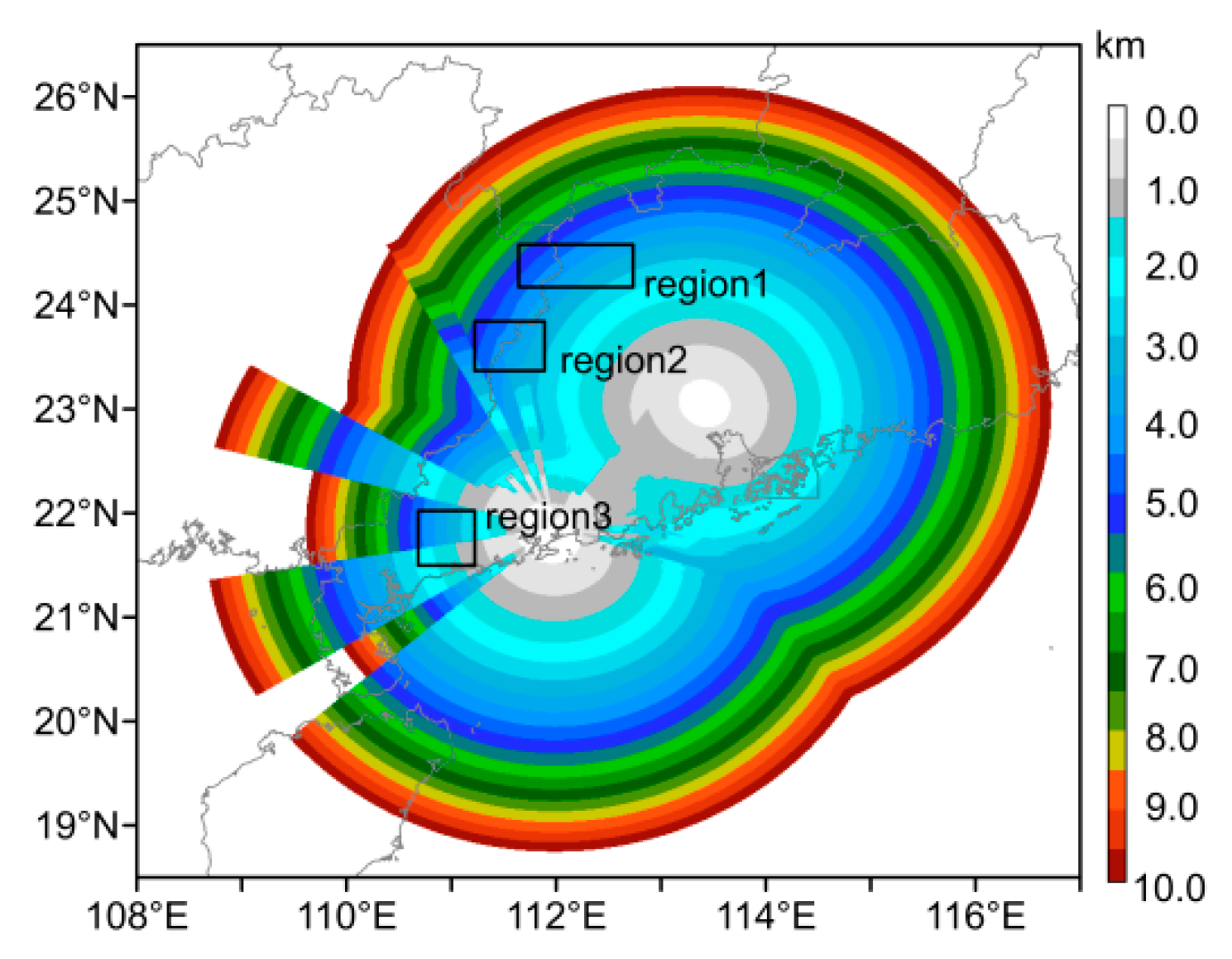
2.1.1. Beam Blockage Situation of Polarimetric Radars

Guangdong province is dominated by mountains. Its terrain is shown in Figure 1a. The positions of the Guangzhou and Yangjiang radars are shown in Figure 1a,b with black triangles. The beam blockages of the two radars are calculated with the method described by Bech et al. [33], and they are shown in Figure 2. The Guangzhou radar is located in the plain area, and the beams are only slightly blocked (Figure 2a). However, there are many mountains around the Yangjiang radar, and the beams are severely blocked at many azimuthal angles (Figure 2b). The blockages are obvious at many northern azimuthal angles, as well as some eastern and western ones. The highest beam blockage percentage nearly reaches 100%, and Yangjiang radar almost obtains no effective echoes in those azimuthal angles. The blockages are topped at 2.4° tilt of Yangjiang radar at some northern azimuthal angles, which are shown in Figure 2d. If only Yangjiang radar data were utilized to estimate precipitation, there would be obvious underestimation or even no QPE value in some beam blockage regions.

2.1.2. Data and Quality Control Method

S-band single-polarization radars in Guangdong province were upgraded to polarimetric radars in 2016. After the radars were upgraded, the range bin length became 0.25 km, but the scan period remained 6 min. The main specifications are shown in Table 1.
Meanwhile, a series of tests were conducted for the transmitter and the receiver. The difference between the expected value and the measured value of the radar constant is calculated based on the radar transmit power and the radar equation, and the difference is corrected in real time. The transmitter is calibrated in this way. The receiver is calibrated with built-in testing and sun-calibration method. These tests indicated that ZH accuracy is better than 1 dB, meeting the requirements for QPE. ZDR is also calibrated with vertical pointed calibration method before the radar operation.
A quality control procedure must be applied to polarimetric radar data before radar mosaic construction and precipitation estimation. Firstly, ZDR is smoothly filtered along the radial direction to reduce random fluctuations. The smoothing range bin number M depends upon the ZH value. The value of M is as follows:
M = { 3 Z H 45   dBZ 5 35   dBZ Z H < 45   dBZ 7 Z H < 35   dBZ
Three, five, or seven gates are used in a running average for ZDR based on ZH values. In this way, ZDR is smoothed to various degrees with various reflectivity factors to avoid non-complete smoothing for weak echoes and excessive smoothing for strong ones.
Kalman filtering is used for ΦDP, and KDP is calculated by a linear least squares fit using N samples of the ΦDP [14]. N is the number of consecutive radar bins for the piecewise linear fit, which is adjusted according to three reflectivity factor levels:
N = { 9 Z H 45   dBZ 13 35   dBZ Z H < 45   dBZ 17 Z H < 35   dBZ
This adaptive adjustment is intended to follow steep phase changes in intensive precipitation regions while maintaining a low variation in the estimated KDP in light precipitation regions [13]. Since the range resolution of the radar is 0.25 km, the estimation can tolerate small-scale variability up to 2.25 km under heavy rain and large-scale variability up to 4.25 km under light rain. Moreover, KDP is also smoothly filtered in the same way as ZDR to reduce random fluctuations. Besides this, the data influenced by radio frequency interference have been identified and eliminated with the method proposed by Wen et al. [34].
During May to June 2016, nine rainfall events were observed by the two radars and the rain gauges around them (Table 2). The rain gauge stations in Figure 1b are all less than 300 km from either radar. Gauges used in this study are tipping bucket rain gauges. The resolution of the rain gauge data is 0.1mm, and the data are received every one minute. In this study, the data from these gauges are accumulated in an hour separately to evaluate the QPE performances. The gauge data are also quality controlled with method proposed by Gou et al. [9]. The quality control for gauge data is mainly carried out by comparing the spatial consistency of gauge data. In general, the rainfall data of gauge stations should not be very different from that of several nearby stations. Once it exceeds a certain range, the rainfall data of this gauge station is considered abnormal and this isolated extreme data needs to be removed.

2.1.3. Analysis of Polarimetric Radars Data Consistency

The radars’ data consistency needs to be confirmed prior to construction of the radar mosaic. To minimize the influence of partial beam blockages, only the narrow black region between the Guangzhou and Yangjiang radars (Figure 2) is selected as a common area for radars data comparison. This region falls within 100 km of the two radars. Rainfall events listed in Table 2 occurring in Guangdong Province are selected for data comparison. Despite the small size of the selected area, extensive data are available for effective comparison.
After the quality control procedure is applied to the two radars’ data, the consistency between them is analyzed. The two radars’ CAPPI (2 km) data are collected for comparison, and the frequency distributions of ZH, ZDR, and KDP are shown in Figure 3. The diagonal lines are equal lines. It is apparent that the three polarimetric parameters are basically distributed near the diagonal lines. The average differences are 0.2555 dB (ZH), 0.0061 dB (ZDR), and 0.0058 °/km (KDP), respectively. The standard deviations of the differences are 4.4848 dB (ZH), 0.3527 dB (ZDR), and 0.2380 °/km (KDP), respectively. Considering that there are biases caused when calculating CAPPI (2 km), the two radars’ data are basically consistent, which satisfies the mosaic condition.

2.2. The Key Methods in Polarimetric Radar Mosaic QPE Algorithm

In the polarimetric radar mosaic QPE algorithm, precipitation is estimated with the mosaic hybrid scan data. It should be noted that the main purpose of the radar data mosaic in this study is to estimate precipitation. The hybrid scan mosaic algorithm used in this study differs from that of the three-dimensional mosaic. The details of the polarimetric radar mosaic QPE algorithm are described below.

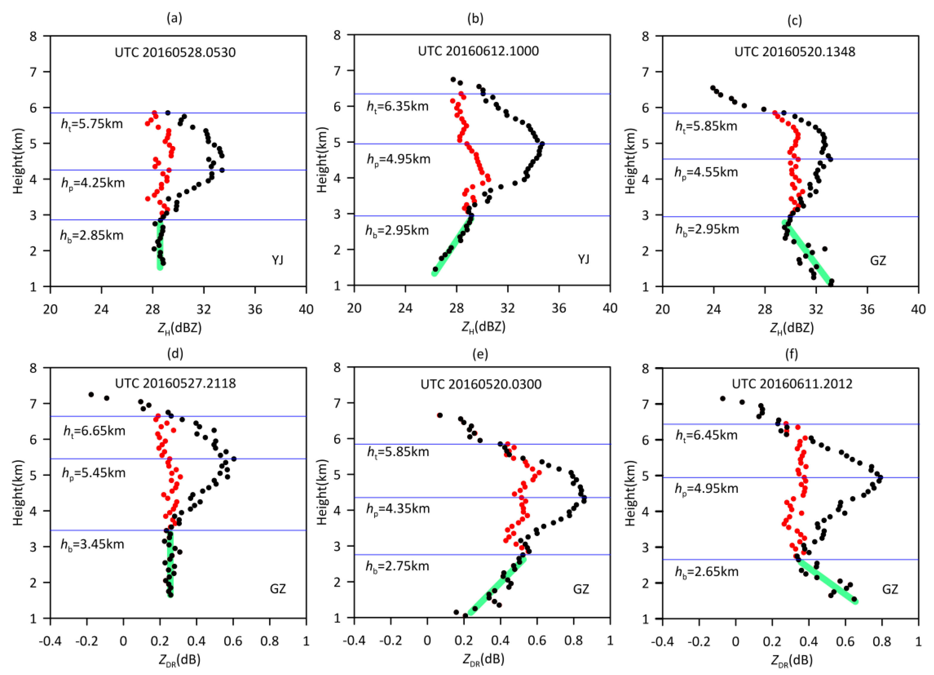
2.2.1. BB Correction

When data from different radars are mosaicked in a grid, the heights of the data are different. Some of them may be in the melting layer. Their data quality is obviously influenced by BB. Therefore, BB correction is necessary in the radar mosaic QPE algorithm.
BB is caused by the melting ice particles; it affects polarimetric radar data, leading to an increase in ZH, ZDR, and KDP, and a decrease in ρHV [25,26]. These changes can make QPE performances uncertain. It is necessary to correct these changing data; however, most previous studies have only corrected ZH to improve QPE performance. In fact, there are some other relations between polarimetric parameters and rain rate R for estimating precipitation in the polarimetric radar QPE algorithm. Besides ZH, some other radar data (such as ZDR and KDP) also need to be corrected. Although ρHV is not directly used to calculate precipitation, it is very sensitive to mixed-phase precipitation particles and can be used to detect BB height. For BB correction, convective and stratiform precipitation echoes are first segregated, then the BB height range is identified, and finally the data are corrected after the vertical profile model is established.
(a) Convective and stratiform precipitation segregation
The composite reflectivity factor (CR) and vertically integrated liquid water content (VIL) are chosen to segregate the convective and stratiform precipitation. Convective precipitation is identified based on that CR > 50 dBZ or VIL > 6.5 kgm−2 [23,35]. Otherwise, the precipitation is classified as being stratiform.
(b) BB height range identification
Once the precipitation type is determined, the following steps are performed only for stratiform precipitation. The apparent vertical profile of data (AVPD) is obtained according to the stratiform precipitation data. The word “apparent” indicates the beam broadening effects in the vertical profile. When a radar observes echoes at a long distance, the height of the vertical profile will be increased due to beam broadening. Therefore, it should be noted that the obtained BB top height will be higher than the “truth”; however, since the statistics and correction of the data are both affected by beam broadening, the data correction is reasonable as long as the data at BB bottom height are correct. This method has been verified for ZH correction in several studies [23,24].
Since ZDR, KDP, and ρHV are unreliable when SNR of the polarimetric radars in Guangdong is below 20 dB [16,32], AVPDs are collected via the ZQ10 method [23] used for ZH with the added condition that the data collected here must have an SNR > 20 dB to ensure high-quality. The AVPD frequency distributions of ZH, ZDR, KDP, and ρHV (shown in Figure 4) are obtained from the Guangzhou and Yangjiang radar data according to the nine rainfall events listed in Table 2. High frequencies indicate that data are concentrated, and show the same feature of most profiles. AVPDs of ZH and ZDR have the same obvious BB feature: the frequencies are very high in the peak-value region, meaning that a large number of data affected by BB become larger than the data near the ground. The same feature provides the basis for the AVPD model. Although the AVPDs of KDP also show that data affected by BB become larger than data near the ground, data points in the peak-value region are more dispersed than those of ZH and ZDR, which poses a challenge for KDP correction in BB. There is a strange profile in the high altitude of the ρHV AVPDs because ρHV does not go back close to unity in ice. There are two possible reasons for the strange profile of ρHV in the high altitude. One reason is the ice mixed with rain. The other one is the SNR with too small value. The reflectivity of the ice in the high altitude is small, and its SNR is also small. The SNR has an obvious influence on ρHV of the polarimetric radars in Guangdong. When the SNR becomes small, the quality of ρHV becomes bad [16,32]. Although only data corresponding to SNR > 20 dB are collected to obtain AVPD of ρHV, the SNR of the ice in the high altitude is smaller than that in the low altitude, and may be close to 20 dB. Therefore, it is the small SNR that makes the ρHV profile strange in the high altitude where pure ice exists.
An ideal AVPD model for ZH, ZDR, and KDP is established based on the same feature of frequency distributions, and it is shown in Figure 5. It can represent most AVPDs of ZH, ZDR, and KDP. The main height parameters include BB top height (ht), BB bottom height (hb), and BB peak height (hp).
The main height parameters must first be identified to obtain the ideal AVPD model. The height of 0°C is read from the sounding data, and the BB peak in AVPD is obtained by searching the maximum value of data around the 0 °C height. The BB top is obtained by searching the first inflection point above the BB peak in AVPD.
It is very important to identify the BB bottom height, because the correction factor is calculated with reference to hb. However, the bottom data of ZH, ZDR, and KDP are scattered, while the bottom data of ρHV are very concentrated (see Figure 4). Most bottom ρHV data are concentrated above 0.975, which is helpful for identifying hb. Therefore, the method used in the MRMS system that identifies hb by searching for the first inflection point of ZH is not used in this study [23,24]. Instead, ρHV is used to identify hb. ρHV is searched from hp down; when the value change rate of ρHV is approximately zero, its height is hb, meaning that ρHV is basically stable. When ρHV is stable, the phase of the hydrometeors is basically unchanged. What’s more, it should be noted that most precipitation particles at the BB bottom height are liquid particles, so ρHV must be larger than a threshold value, which is set to 0.975 in this study. A similar method proposed by Qi et al. [36] that uses ρHV to detect hb proves to perform better than that using ZH (such as ZQ10) on tests for three heavy precipitation events from different geographical regions and seasons in the United States, which indicates the feasibility of the proposed method in this study.
(c) AVPD modeling and BB correction
The height parameters, ht, hb, and hp, are used to derive a parameterized, two-piece-linear AVPD model. One piece is between the BB top and the peak and another is between the BB bottom and the peak. The slope values α and β are fitted using two data sections according to a least squares method. The correction factor Da(h) is obtained based on the established AVPD model, which is shown as follows:
D a ( h ) = { α [ h ( r ) h p ] + β [ h p h b ] h p   <   h ( r ) h t β [ h ( r ) h b ] h ( r ) h p .
The corresponding data are corrected as follows:
D c ( φ , 0 ) = D o ( φ , h ) D a ( h )     ( φ , h ) B B A ,
where r, φ , and h are the range, azimuth, and height of the beam axis at a given gate, respectively. D o ( φ , h ) and D c ( φ , 0 ) are the raw and corrected data, respectively. In this study, these data include ZH (dBZ), ZDR (dB), and KDP (°/km).
In the real time applications, these three steps are implemented for one radar volume scan data to obtain its AVPD model at every volume scan period. The parameters of the AVPD model adapt with time, and the BB correction is applied in real time. It should be noted that the AVPD model is only derived and applied to the BB affected area (BBA) rather than to the whole radar coverage.
The above method is based on a specific set of data. They are from the rainfall events occurred in the warm season of Guangdong, China. The similar environment of these events makes AVPD relatively stable. This provides a guarantee for the effectiveness of this BB correction method, especially for warm season rainfall. Although AVPD changes due to microphysics and changing events, the parameters of the AVPD model adapt with time. These changing parameters can help mitigate correction biases due to the changing AVPD. However, when the environment changes largely, such as when a winter stratiform rain behind a cold front occurs, the ideal AVPD model shown in Figure 5 may be very different. This correction method may not be useful then. Further improvements can be made in the future studies. This BB correction method proposed in this study is better used for warm season rainfall for now.

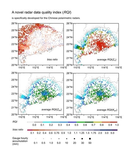
2.2.2. Radar Data Quality Index and Polarimetric Radar Mosaic Algorithm

The hybrid scan data for the single radar need to be obtained before constructing the radar mosaic. The basic principle of the hybrid scan is to select the ground-clutter-free data to be as low as possible from the ground without obvious blockages. This differs from the three-dimensional mosaic, which aims to obtain data at different heights, such as CAPPI. In this study, data from the lowest tilt with beam blockages of <0.3 and ρHV > 0.7 are chosen as the hybrid scan data based on this principle, to avoid complex terrain influences.
The hybrid scan data can be obtained with the above method and then used to construct the radar mosaic. Although BB correction has been applied to the data, it is still important to know the radar data quality. Only when the data quality is known quantitatively, high-quality data can be selected to obtain the high-quality mosaic data. Therefore, a radar data quality index (RQI) is proposed in this study to quantitatively describe the data quality. It is referenced from a radar QPE quality index proposed by Zhang et al. [37] (hereafter Z11). Their index is proposed to identify and estimate the influences of partial beam blockage and BB upon QPE in their study. In fact, the QPE accuracy is mainly related to radar data quality and the relationship of radar parameters and rain rate. On the assumption that this relationship is accurate, radar data quality also can represent the accuracy of QPE. Therefore, in addition to representing data quality, RQI proposed in this study is expected to reflect QPE accuracy. This topic is also discussed in Section 4.2.
RQI is governed by many factors, including partial beam blockages, BB, BB correction performance, SNR, and the non-precipitation echoes. BB correction performance and SNR are the factors not considered in other studies. However, these factors are important to the polarimetric parameters. The BB correction performance influences the data quality after the correction is applied to these data. If this factor is not considered, the corrected data cannot be used in a correct way in the BBA. Besides this, the qualities of Chinese polarimetric parameter ZDR, KDP, and ρHV are obviously influenced by SNR [16,32]. Therefore, SNR is a key factor which need be considered when Chinese radar data are used. All the above factors are reflected in RQI with four indexes. They are introduced as follows.
RQIblk is an index proposed in Z11 study. It is still used here, shown as follows:
R Q I blk = { 1 b l k 0.1 ( 1 b l k 0.1 0.4 ) 0.1 < b l k 0.5 0 b l k > 0.5 ,
where blk indicates the beam blockages. The influence of partial beam blockages upon radar data quality can be represented by blk. RQIblk is the index affected by partial beam blockages and is calculated based on blk. At any given time, the quality of radar data is generally worse in complex terrains (large blockages) than in flatlands (no blockages). Therefore, when blk is large, the RQIblk is set to small, and vice versa. The model of RQIblk is shown in Figure 6a.
RQIhgt is the other part of RQI in the Z11 study, and this index is affected by BB. However, in the Z11 study, RQIhgt was calculated based on the assumptions that the thickness of BB is 700 m and that the data below h0c-700 (m) are not affect by BB. This is obviously not accurate, so RQIhgt is improved based on hb according to the observed BB. In addition to the thickness of BB, a height scale factor is also a fixed value in the Z11 study, meaning that the BB correction performance is not considered. In this study, Hsf (m) is a height scale factor that changes with BB correction performance and is used in the new RQIhgt. It is shown as follows:
R Q I hgt = { 1 h b > 0 h a < h b e x p ( ( h a h b ) 2 H sf 2 )   h b > 0 h a h b e x p ( h a 2 H sf 2 )   h b < 0 ,
H sf = ( 2.5 R N D ) × 1000 ,
R N D = | N D | N D f i x ,
N D = a v e B B a v e u B B | a v e u B B | ,
where ha(m) is the height of the beam axis, aveBB is the average value of data in BB, aveuBB is the average value of data under BB, and ND is the normalized difference between aveBB and aveuBB. ND represents data quality in BB. When ND is 0, the data in BB and under BB show good consistency. When ND is larger (resp. smaller) than 0, the average value of data in BB is larger (resp. smaller) than that under BB. The smaller the absolute value of ND, the better the BB correction performance is. The average value of data in BB and under BB are used to calculate ND, because it makes the calculation of RQIhgt simple and feasible, and ND can basically reflect the performance of BB correction to make the RQIhgt more reasonable. However, computing an average value under the BB will mask signature of microphysical processes that influence precipitation rate. In fact, some data under BB are not invariable, and have different changing trends. The changing trends of data under BB are discussed in Section 4.1. NDfix is a fixed value of ND, which can stand for the average ND before BB correction. The default NDfix of ZH is 0.07, that of ZDR is 0.5, and that of KDP is 0.8. These are values derived from the nine rainfall events in this study. These values can be treated as the empirical values of radars in Guangdong. If the NDfixs are used for other radars, the values of them can be adjusted according to the characteristics of local radar. RND is the ratio of |ND| and NDfix, which can represent the BB correction performance. It is used to calculate Hsf. The equation of Hsf is established empirically to form the curves in Figure 6b. Hsf is limited in the range (500–2500) to avoid the abnormal value. The black lines 1, 2, and 3 in Figure 6b represent RQIhgt with Hsf values of 500 m, 1500 m, and 2500 m, respectively.
The quality of radar data is generally worse in areas with low freezing levels than those with high freezing levels. The freezing levels are related to the height of the beam axis. Therefore, RQIhgt is also influenced by the position of the beam axis relative to the BB bottom height, hb. When the beam axis is below hb, rain drops cannot be frozen and the value of RQIhgt is 1; the higher the beam axis is relative to hb, the less accurate that the data are. In addition, when the ambient temperature is too low, h0c is very close to the ground and it is difficult to identify hb, which is denoted by hb < 0 in formula (6), and only ha is used to calculate RQIhgt. The greater the height, the less accurate the data.
Z11 focused on the QPE of single-polarization radars, for which an RQI that only includes RQIblk and RQIhgt can satisfy requirements. However, radar data quality is also influenced by SNR and the non-precipitation echoes, especially for the polarimetric parameters ZDR, KDP, and ρHV. SNR and the non-precipitation echoes are represented by snr (in linear scale) and ρHV, respectively. The index takes the form of a Gaussian function because it can represent the gradual change of radar data quality affected by snr or ρHV. The snr and ρHV are x-axis variables [38]. The value of the Gaussian function gradually decreases by controlling the threshold value. RQIsnr and RQIΡHV are shown as follows:
R Q I snr = e x p [ 0.69   ×   ( s n r * s n r ) 2 ] ,
R Q I ρ HV = { 1 d a t a : Z H , ρ HV e x p [ 0.69 × ( 1 ρ HV Δ ρ HV * ) 2 ]     d a t a : Z DR , K DP ,
where snr * and ΔρHV * are the threshold values of the Gaussian function. The SNR * (corresponding to snr *) of ZH is 0dB and those of ZDR, KDP, and ρHV are 25 dB. The Δ ρHV * values of ZDR and KDP are 0.1. RQIsnr is the index affected by SNR, and is calculated based on snr. Some studies [16,32] have shown that when the SNR of the polarimetric radars in Guangdong falls below 20 dB, ρHV, ZDR, and KDP become unreliable. Therefore, the index of RQIsnr is set to 0 when the SNR is below 20 dB, as can be seen from the model shown in Figure 6c. RQIΡHV is the index affected by the non-precipitation echoes, which is calculated based on ρHV. When precipitation echoes are mixed with the non-precipitation echoes, ρHV becomes smaller, and the qualities of the other polarimetric parameters become worse. When ρHV is under 0.7, the echoes are non-precipitation echoes [16], so the RQIΡHV of ZDR and KDP is set to 0. The RQIΡHV model of ZDR and KDP is shown in Figure 6d. Ground echo suppression has been made for ZH, and echoes corresponding to low ρHV are treated in a certain way by the QPE algorithm, so the index of ZH is set to 1. ρHV is the value reflecting non-precipitation echoes. Since it does not make sense to use ρHV to evaluate ρHV, the index of ρHV is also 1.
The simple linear and exponential functions are chosen to represent these indexes because of their computationally efficiencies for real-time implementation. All of the above indexes should be taken into account to quantitatively evaluate the polarimetric data quality; RQI is calculated as follows:
R Q I = R Q I blk × R Q I hgt × R Q I snr × R Q I ρ HV .
Thus, RQI can represent the quality of radar data under the influence of partial beam blockages, BB, and BB performance, SNR, and non-precipitation echoes; thus, it can be used for data quality comparison. Based on this comparison, low quality data can be identified and eliminated. The polarimetric radar data mosaic algorithm flowchart is shown in Figure 7.
The RQI of the lowest data (RQIlowest) is used as a standard value for comparison with the RQI of the other data in the same grid. The data point with an RQI value under RQIlowest − 0.2 or equal to 0 are treated as low quality data and eliminated. The number of the data points remaining determines how the mosaic data are obtained. If no data are left, the mosaic data of this grid would be flagged as suspicious. If only one data point is left, then this data point is selected to be the mosaic data for this grid. If there are two data points left, they are merged to obtain the mosaic data. For three or more data points left, only the three with the largest RQI values are merged.
Data merging is performed according to the following formula:
M o s a i c   D a t a = i = 1 n w L i × w H i × R Q I i × D a t a i i = 1 n w L i × w H i × R Q I i ,
w L = exp ( d 2 / L 2 ) ,
w H = exp ( h 2 / H 2 ) ,
where wL and wH are the horizontal and vertical weighting factors, respectively, d is the horizontal distance between the analysis point and the radar, h is the height of the radar bin, and L and H are the scaling factors with default values of 100 km and 2 km, respectively. Mosaic Data is the final mosaic radar data, and n is the mosaic radar number. In addition to the larger weighting given to the data that are closer to the ground and to the radar, the data with higher quality are also more heavily weighted in calculating the mosaic data, because RQI is considered as a weighting factor. This makes the mosaic data more reliable.
Although RQI is proposed for the Chinese radars in this study, it can be used in different regions and different seasons with different coverages. One thing that should be noted is that the default values of some variables need to be adjusted according to the characteristics of local radar.

2.2.3. Polarimetric Radar Mosaic QPE Algorithm

The mosaic data can be obtained based on the above algorithm. Firstly, the BB correction is applied to the polarimetric radar data, and then RQI is calculated and used to obtain the mosaic data. Finally, the mosaic data is used to estimate precipitation. The flowchart of this new QPE algorithm is shown in Figure 8.
The QPE algorithm mainly follows the polarimetric radar QPE algorithm proposed by Zhang et al. [12] (hereafter Z18). The Z18 algorithm performs well for rainfall events occurring in Guangdong province; however, an SNR > 20 dB is simply used to distinguish ZDR and KDP values of high quality from those of low quality in Z18 algorithm. The Z-R relationship is used to estimate precipitation when ZDR and KDP have low quality. Although the same strategy is applied to the QPE algorithm, the RQIs of ZH, ZDR, and KDP are used to determine whether the Z-R relationship is suitable for estimating precipitation in the new QPE algorithm. This is because RQI can more accurately represent the quality of data than SNR. When RQI(ZH) − RQI(ZDR) > 0.5 and RQI(ZH) − RQI(KDP) > 0.5, the quality of ZH is much better than that of ZDR and KDP, thus the Z-R relationship is used to estimate precipitation.
Data in BBA are different from data in other areas, and BB correction performances of different data are different. These all make estimating precipitation in the BBA more special. The QPE algorithm in the BBA needs to be different from the algorithm in the other areas, and it is studied here. Firstly, the influences of corrected ZH, ZDR, and KDP upon the QPE in the BBA are studied. In order to study these influences, average raw and corrected data in the BB are used to estimate precipitation, and precipitation estimated based on data at the BB bottom height is treated as the “truth” value to evaluate them. As statistical indicators of the QPE performance in this study, the correlation coefficient (CC), root mean square error (RMSE), normalized relative bias (NB), normalized absolute error (NE), and bias ratio of radar-estimated rainfall to the “truth” value of rainfall are obtained:
C C = i = 1 n ( Q P E i r a d a r Q P E i r a d a r ¯ ) ( Q P E i t r u t h Q P E i t r u t h ¯ ) i = 1 n ( Q P E i r a d a r Q P E i r a d a r ¯ ) 2 i = 1 n ( Q P E i t r u t h Q P E i t r u t h ¯ ) 2 ,
R M S E = i = 1 n ( Q P E i r a d a r Q P E i t r u t h ) 2 n ,
N B = i = 1 n ( Q P E i r a d a r Q P E i t r u t h ) i = 1 n Q P E i t r u t h × 100 ,
N E = i = 1 n | Q P E i r a d a r Q P E i t r u t h | i = 1 n Q P E i t r u t h × 100 ,
b i a s   r a t i o = i = 1 n Q P E i r a d a r i = 1 n Q P E i t r u t h ,
where QPE is the rainfall derived from either radar or “truth” value, an overbar represents a mean value, n is the number of QPEitruthQPEiradar pairs, RMSE has the same units as QPE, and NE and NB are both percentages. A bias ratio value larger (resp. smaller) than one indicates overestimation (resp. underestimation).
The evaluated statistical scores for radar QPE based on raw/corrected data in the BB are shown in Table 3. It is obvious that results derived from the corrected ZH and ZDR values are better than those derived from the corrected KDP in terms of NE and NB. This indicates that the corrected ZH and ZDR values are more suitable for estimating precipitation in the BBA than the corrected KDP. Therefore, only corrected ZH and ZDR are used to estimate precipitation in the BBA in this study.
It should be noted that BB correction cannot make data in BB equal to data under BB. The BB correction performance can be good or bad; when the ZDR correction performance in BB is bad or much worse than the ZH correction performance in BB, the Z-R relationship becomes the only choice for estimating precipitation. When |ND(ZDR)| > 0.2, the quality of ZDR is considered to be very low, and the ZDR correction performance in BB is bad. When RND(ZH) − RND(ZDR) < −0.2, the BB correction performance of ZDR is considered to be much worse than that of ZH. Therefore, when |ND(ZDR)| > 0.2 or RND(ZH) − RND(ZDR) < −0.2, the Z-R relationship is used in the QPE algorithm. These values used in this study are also empirical values, which can be adjusted according to the characteristics of local radar.
In addition, ZH < 20 dBZ and ρHV < 0.8 are treated as the characteristics of the clear-air echo; there is no precipitation. The rest of the QPE algorithm flowchart follows the Z18 algorithm, which is not introduced in this study.

3. Results

3.1. Performances of BB Correction

ND can represent data quality in BB, so it can also reflect the data correction performance in BB. The ND frequencies of ZH, ZDR, and KDP derived from the nine rainfall events listed in Table 2 are shown in Figure 9; the gray histograms are derived from corrected data in BB, and those with black lines outside are derived from raw data in BB. The NDs of ZH, ZDR, and KDP all approach zero after BB correction, indicating good correction performance for the whole dataset. The average NDs of the corrected ZH, ZDR, and KDP values are 0.013, −0.026, and −0.241, respectively. The average NDs of ZH and ZDR are all much closer to zero than that of KDP. The main ND frequency distributions of corrected ZH and ZDR are mostly Gaussian; however, that of the corrected KDP is not. These all indicate that the BB correction performance of KDP is not as good as that of ZH and ZDR. This is also why KDP is not suitable for estimating precipitation in the BBA.
Here we describe a case that reflects the BB correction performance of ZH, ZDR, and KDP. The original and corrected mosaic data at 20:54 on 15 June 2016 are shown in Figure 10. This is a squall line rainfall event. The small value of ρHV in the stratiform region behind the convective echoes of the squall line is obviously caused by BB, which is marked with a black circle in Figure 10a–h. Blue in Figure 10h represents BBA. Most of the BBA is in the black circle. The values of the corrected mosaic ZH, ZDR, and KDP in the circles have been reduced compared with the original data.
The BBA mainly falls within the detective range of the Guangzhou radar. The AVPDs of ZH, ZDR, KDP, and ρHV, as derived from the Guangzhou radar, are shown in Figure 10. Black dots indicate original observations and red dots indicate corrected values. It can be seen that the original values of ZH, ZDR, and KDP show obvious enlargement at a height of around 5 km. The thickness of the BB is larger than the true value due to the beam broadening effect, especially at the BB top height, which may deviate from the true value. However, it does not affect the correction of polarimetric radar data. The large values of the original data at around 5 km become close to the ground data values after correction. However, the discontinuity of the original KDP vertical profile leads to discontinuity in the corrected KDP vertical profile. BB correction for ZH and ZDR performs better than that for KDP. Although the AVPD frequency distribution of KDP follows the ideal AVPD model, certain vertical profiles of KDP sometimes cannot follow the ideal AVPD model well; this is why the BB correction performance of KDP is not very good. This also influences the performances of estimators using the corrected KDP (Table 3). Therefore, KDP should not be used to estimate precipitation in the BBA even after correction.
BB correction mitigates the increase of observed data due to the melting of ice particles and can therefore improve QPE performances. However, it is impossible to tell whether this will mitigate the overestimation or underestimation of precipitation, since ZH is positively correlated with R while ZDR is negatively correlated with R in the rainfall estimators. ZH and ZDR in BB both increase before correction, but the change of R is related to the proportion of the two parameters used to estimate precipitation and the contributions of the two parameters to R. The QPE performances in the BBA are further analyzed in Section 3.3.

3.2. Results of the Polarimetric Radar Data Mosaic

On the hypothesis that echoes produced by precipitation exist in each altitude layer and that there is no noise signal, the ideal mosaic heights of the Guangzhou and Yangjiang radars are shown in Figure 11. Some radial vacancies occur around the radar due to beam blockages for lower tilts at these azimuthal angles. In the hybrid scan strategy, the data from the lower tilt are replaced by those from the upper tilt. Their height differences result in radial vacancies. In the overlap area of the two radars, most mosaic height data are also calculated by the data mosaic formula (13); however, the severe beam blockages of the Yangjiang radar lead to a few irregular heights in this area.
The mosaic ZH, ZDR, KDP, and ρHV are obtained via the proposed mosaic algorithm using the data observed by the Guangzhou and Yangjiang radars at 5:00 on 20 May 2016. The mosaic data and their corresponding RQIs are shown in Figure 12.
All RQI data are distributed with echoes and are larger than zero only where echoes exist. The size of the RQI(ZH) with a high value (e.g., >0.9) is the largest. It is mainly influenced by the height of the radar data, since when the height is larger than a given value, RQIhgt decreases rapidly. The distributions of RQI(ZDR) and RQI(KDP) behave similarly. The only difference between them is RQIhgt because of the different BB correction performances. The distributions of RQI(ZDR), RQI(KDP), and RQI(ρHV) are all seriously influenced by SNR. The ranges of RQI(ZDR), RQI(KDP), and RQI(ρHV) are almost the same as the range of SNR larger than 20 dB (shown in Figure 12i). In addition, RQI(ZDR) and RQI(KDP) are also influenced by ρHV. Although the SNR is large in areas near the two radars, RQI(ZDR) and RQI(KDP) are small because of the small value of ρHV, which corresponds to ground clutter.
Only in the area where RQI(ZDR) and RQI(KDP) are larger than zero do ZDR and KDP have a chance to participate in estimating precipitation alongside ZH. In the other areas, ZH is the only reliable estimation parameter, especially in areas where RQI(ZH) is larger than 0.9. It seems that the red areas of RQI(ZH) can indicate effective QPE areas, and this will be analyzed via the QPE performance in Section 4.2.

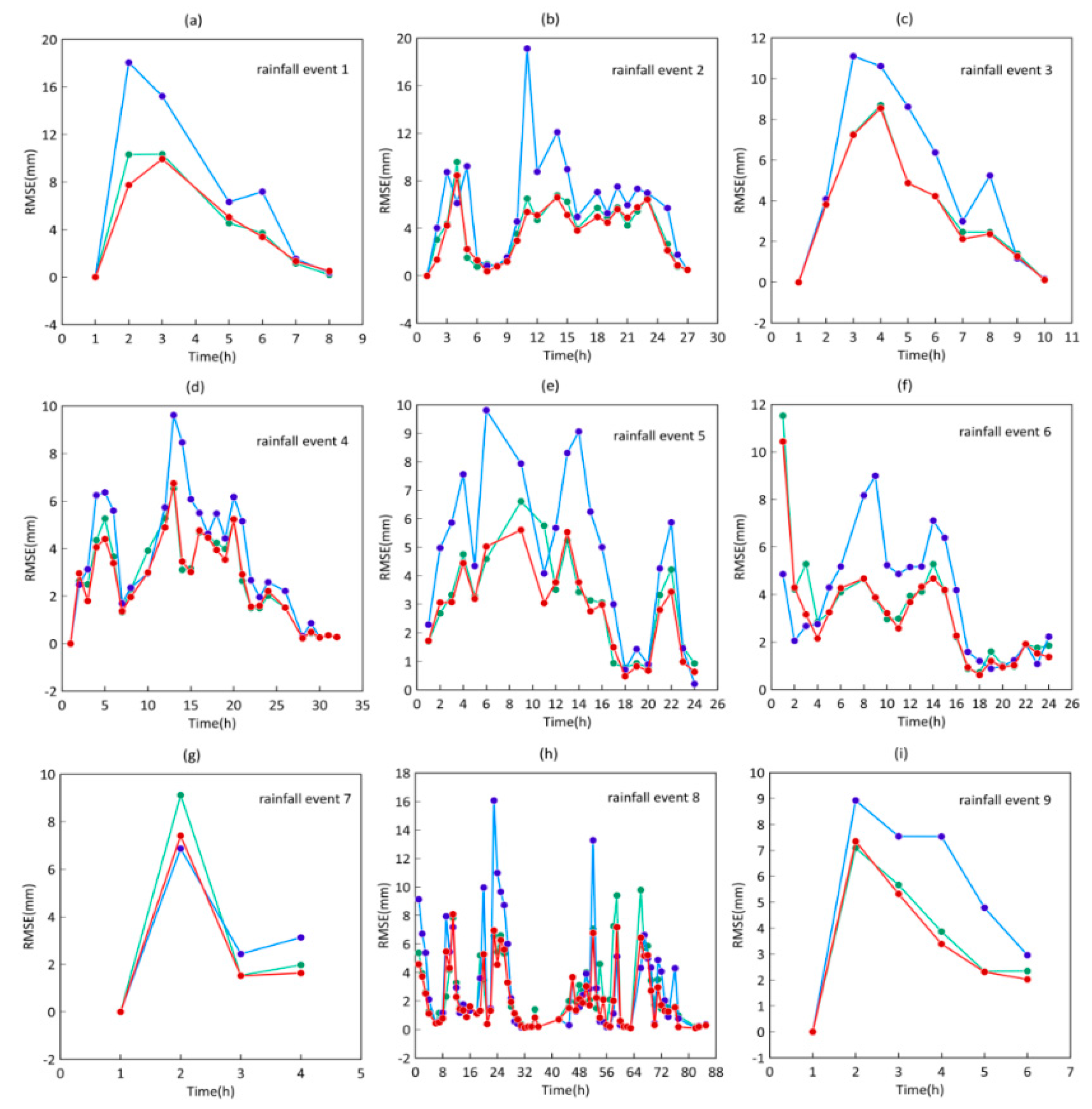
3.3. Results of Polarimetric Radar Mosaic QPE

The radar mosaic data are obtained from the nine rainfall events listed in Table 2, and used to estimate precipitation based on the mosaic QPE algorithm proposed in this study. QPE (spatial resolution: 1 km × 1 km) is computed in the detective range of the two radars, but it is evaluated limited in the common region of the two radars. In order to see the QPE performances on a large scale, especially the performance in the radar beam blocked area, they are evaluated with rain gauge data from within 300 km of each radar. The size of this evaluation region is about 169,821 km2. The rainfall accumulations measured at the rain gauge station are used as “true” accumulations. The rainfall accumulations from the radars are accumulated by using the data of every volume scan period on the assumption that the rain rate for the duration of the volume scan is continuous. The average radar-estimated precipitation of the nine grids nearest the rain gauge station is used to evaluate the QPE performance. Since the minimum rainfall measurement of the rain gauge is 0.1 mm, only rainfall measurements exceeding this value were used for evaluation. There are 51,985 sample pairs of QPE-gauge data used for evaluation in this region. The distributions of the bias ratios derived from the evaluation results of radar mosaic QPE and the two-radar QPE are shown in Figure 13.
Due to the partial beam blockages caused by the complex terrain, the Yangjiang radar QPE is significantly underestimated in the beam blockage directions, and only achieves good estimation performance in a small area close to the radar (Figure 13c). Since the western part of the evaluation area is far from the radar, the beam axis height of the Guangzhou radar is very high when observing this area, such that the beam may overshoot the echo top or only a weak echo can be observed. This leads to clear underestimation of Guangzhou radar QPE in the western evaluation area (Figure 13b). The radar mosaic QPE products take advantage of the QPE products of both radars. Not only does this avoid severe underestimation of Yangjiang radar QPE in partial beam blockages areas, it also avoids underestimation caused by the beam overshooting the echo top far from the Guangzhou radar. This indicates the advantage of the radar mosaic (Figure 13a).
The bias ratio distributions clearly show that the radar mosaic can effectively mitigate errors caused by partial beam blockages and the beam partially overshooting cloud tops when using single radar. To quantitatively analyze the other advantages of radar mosaic QPE, only data from rain gauge stations within 180 km of each radar which are in the inner region of the black spindle shape (Figure 13) are selected to calculate the evaluated statistical scores of the radar mosaic and the two single radar QPEs. The size of this evaluation region is about 36,251 km2. There are 12,694 sample pairs of QPE-gauge data used for evaluation in this region. The scores are listed in the Table 4. Although the NB of the radar mosaic QPE is not very good, it still falls within acceptable limits. The QPE performance of the radar mosaic is better than those of either single radar in terms of CC, RMSE, and NE. After the radar mosaic is constructed, the RMSE and NE of QPE are reduced by at least 5.29% and 5.59%, respectively. The main advantage of radar mosaic is that it can improve QPE performances in the blocked area and the area far from the radars compared to the single radar. However, without considering the error caused by partial beam blockages and the beam partially overshooting cloud top, the performance of polarimetric radar mosaic QPE is still better than that of single polarimetric radar QPE. This indicates that the polarimetric radar mosaic QPE algorithm proposed in this study can take advantage of all radars to obtain mosaic data which can be better used to estimate the ground precipitation.
In order to know the performance of the radar mosaic QPE in real time, a near real-time statistics of RMSEs derived from the nine rainfall events are shown in Figure 14. RMSEs derived from radar mosaic QPE are smaller than the other two kinds of RMSEs at most time. CCs, NEs, and NBs are not shown here. These three statistical indicators derived from Yangjiang radar QPE are still worst at most time because of the obvious beam blockage. These three statistical indicators derived from radar mosaic QPE and Guangzhou radar QPE performs similar, but radar mosaic QPE performs a little better than Guangzhou radar at most time. These indicate there is a near real-time improvement when the radar mosaic QPE algorithm is applied. This is important for the operational application of the radar mosaic QPE algorithm.
In addition, BB correction is applied to ZH, ZDR, and KDP in the polarimetric radar mosaic QPE algorithm. In order to analyze the effect of BB correction upon QPE, the algorithm without BB correction and the algorithm proposed in this study are respectively used to estimate precipitation. The evaluation results are shown in Figure 15.
The heights of regions 1, 2, and 3 in Figure 15 are about 3–5 km from the mosaic height map shown in Figure 11. The data at these heights are always influenced by BB during May to June in Guangdong province. From the evaluation results, it can be seen that the original polarimetric radar QPE algorithm with ZH and ZDR still overestimates precipitation in the BBA. BB is known to lead to a significant increase in ZH and ZDR. Although the increase in ZDR can reduce the QPE value, the overestimated results indicate that the increase of ZH has a larger effect upon QPE than does the increase of ZDR. According to the statistics, the percentage of precipitation estimated from ZH, ZH + ZDR, KDP, and KDP + ZDR are 90.45%, 7.92%, 0.29%, and 1.34%, respectively. This indicates the RQI of ZH is better than ZDR and KDP, and the rainfall estimators use ZH more often than they use ZDR. Therefore, the algorithm without BB correction still overestimates precipitation in BBA.
The QPE performances of the two algorithms in regions 1, 2, and 3 are evaluated, and the results are shown in Figure 15b,e. The overestimation in these regions has been mitigated as a result of BB correction. After BB correction, NB is reduced from 18.42% to −1.93%. NE and RMSE are also clearly improved, indicating a reduction in absolute error. These results all indicate that BB correction improves the QPE performances in the BBA.

3.4. Sensitivity Tests about the Precipitation Types

The percentages of stratiform precipitation and convective precipitation of these nine rainfall events are 77.60% and 22.40%, respectively. Different percentage of the precipitation types may bring different QPE performances even using the same QPE algorithm. If the precipitation types percentage of these nine rainfall events changes, how the QPE performances would change. In order to solve this question, the influences on QPE caused by percentages of the precipitation types are necessary to be studied.
Some sensitivity tests are performed to see how the evaluated statistics (RMSE, NE, NB) would vary with changing percentages of stratiform and convective. The precipitation in these tests is only mixed with convective precipitation and stratiform precipitation. The pairs of QPE and gauge data are collected from the nine rainfall events and in the area less than 180 km from either radar. They are divided into two groups according to the precipitation types. One is the convective precipitation group, and the other one is the stratiform precipitation group. Two thousand pairs of the QPE and gauge data are selected for one percentage of the precipitation type. For example, if the convective precipitation percentage is 30%, there would be 600 pairs of the QPE and gauge data that are selected from the convective precipitation group at random. There would be 1400 pairs of the QPE and gauge data that are selected from the stratiform precipitation group at random. There are 11 tests with 11 groups of 2000 pairs of QPE and gauge data corresponding to different percentage of precipitation types. The percentages of convective precipitation data are set at 0%, 10%, 20%, 30%, 40%, 50%, 60%, 70%, 80%, 90%, and 100%, respectively, in the 11 tests. There are 11 groups of the evaluated statistics calculated with the 11 groups of datasets.
The results are shown in Figure 16. RMSE changes obviously as the percentage of convective precipitation changes. This is because RMSE is influenced by the rain rate. This feature can be seen from Equation (17). As the percentage of convective precipitation becomes large, the rain rate becomes large and so does RMSE. RMSE ranges from 2.11 mm to 7.34 mm. NE and NB have nothing to do with the rain rate according to Equations (18) and (19), because they are the relative parameters. There are only three tests, in which NE is over 40%. The percentage of convective precipitation is low in these three tests. The worst NB appeared in the first test, in which there is no convective precipitation. These indicate the algorithm proposed in this study is a little less effective in estimating the stratiform precipitation than convective precipitation. However, the values of NE and NB are basically stable in the all 11 tests. NE ranges from 35.25% to 45.83%, and NB ranges from −9.91% to −6.46%. The values of them are acceptable. These results indicate the radar mosaic QPE algorithm proposed in this study can perform well and stably for any type of precipitation occurred in warm seasons.

4. Discussion

4.1. AVPD under BB

BB correction in this study clearly mitigates the increasing effect of ZH and ZDR caused by melting ice particles, causing the average values of ZH and ZDR in BB to approach those under the bottom of the BB. Therefore, the QPE bias in the BBA for all nine rainfall events becomes small, as described in Section 3.3. However, some phenomena still require examination, including the changing trend of data under BB, because they may exert obvious influences upon QPE performance.
Some AVPDs are shown in Figure 17. The green lines represent the changing trends of the ZH and ZDR profiles under BB. The green lines in Figure 17a,d are perpendicular to the horizontal axis, meaning that the averages of ZH and ZDR are basically unchanged with height under the BB. In general, the profiles of ZH and ZDR are basically unchanged under BB, or at least have no discernible tendency to change. However, significant changes sometimes occur in the profiles of ZH and ZDR under BB, as shown in Figure 17b,c,e,f. These always cause some uncertainties in precipitation estimation.
One trend is that average values decrease along as the height decreases, as shown for ZH and ZDR in Figure 17b,e, respectively. The changing rates under BB differ from those between the BB peak and bottom heights. This indicates that their changing mechanisms are different. The other changing tend is that the average values increase as the height decreases, as shown for ZH and ZDR in Figure 17c,f, respectively. The changing trends under BB are complex and their mechanisms are not clear. The precipitation particles change from the ice phase to the liquid phase in BB. The changing trends under BB are probably associated with changing drop size distribution (DSD). It is necessary to study the vertical change of DSD under BB in future work. This study can also be extended to different precipitation regions and different precipitation types to analyze the vertical changes in DSD and polarimetric parameters to obtain more accurate QPE.

4.2. The Relationship between QPE Accuracy and RQI

RQI in this study can represent the influences of the partial beam blockages, BB, BB correction performance, SNR, and the non-precipitation echoes upon polarimetric radar data. In theory, the RQI value can reflect the accuracy of QPE under the above factors. In the Z11 study, the RQI that only reflected the partial beam blockages and BB showed a good correlation with QPE accuracy. This conclusion is also verified by the study of Chen et al. [39]. However, these studies differed from the present one, in that they used only ZH to estimate precipitation, while more polarimetric parameters are used in this study and more factors are considered in our RQI. To study the relationship between QPE accuracy and RQI, the bias ratio and average RQIs of ZH, ZDR, and KDP for the nine rainfall events are shown in Figure 18.
The distribution of the average RQI of KDP is almost the same as that of ZDR, because their values only differ in terms of the BB correction performances, and this difference is very small on average. The average RQI distributions of ZH, ZDR, and KDP show some similar characteristics. Their shapes with colors are all limited by the partial beam blockages and the distance from the radars. The average RQI values of ZH are larger than those of ZDR and KDP. This is because the low SNR and ρHV decrease the RQIs of ZDR and KDP but have little influence upon the RQI of ZH.
A good correlation can be seen between the QPE accuracy and the RQI of ZH from the distributions in Figure 18, as well as the RQIs of ZDR and KDP, despite the values of ZH and ZDR (or KDP) being so different. To quantify their correlation, a new bias ratio is proposed, which is shown as follows:
n e w   b i a s   r a t i o = { b i a s   r a t i o b i a s   r a t i o 1   1 b i a s   r a t i o b i a s   r a t i o > 1 .
The CC between the new bias ratio and the average RQI of ZH (ZDR and KDP) is 0.80 (0.71 and 0.70). This quantitatively verifies the view that there is good correlation between the QPE accuracy and the RQI of ZH (ZDR and KDP). Such correlation exists because the RQI partially models the uncertainties due to the partial beam blockages, BB, BB correction performance, SNR, and the non-precipitation echoes. However, the uncertainties associated with spatially varying drop size distributions still affect the correlation between QPE accuracy and the RQI of ZH (ZDR and KDP), because RQI cannot represent these uncertainties. Based on the good correlation found between QPE accuracy and the RQI of ZH, an effective QPE area can be defined with an RQI of ZH lager than 0.9. QPE performances are evaluated within the radars’ detection range. At the same time, only the QPEs corresponding to the RQIs of ZH larger than 0.9 are used for evaluation, and the performance is basically acceptable in terms of CC (0.83), RMSE (4.00 mm), NE (44.8%), and NB (−2.84%). Therefore, the effective QPE area defined here is reasonable. This area can help in obtaining accurate radar QPE information, which will be beneficial to the application of radar QPE products. Besides this, since there is good correlation between the QPE accuracy and the RQI, RQI can reflect the QPE accuracy to some extent. Therefore, RQI can be used in a weigh function when radar QPE is merged with other precipitation products derived from other different sensors. This is also beneficial to the application of radar QPE products.

5. Conclusions

A new polarimetric radar mosaic QPE algorithm based on RQI was proposed. This algorithm can be used in different regions with the default values adjusted according to the characteristics of local radar. RQI of this algorithm can quantitatively describe the quality of ZH, ZDR, KDP, and ρHV, and is used in high-quality data screening and mosaic data merging. In this algorithm, BB correction is performed to mitigate the increase of ZH, ZDR, and KDP caused by the melting ice particles in the rainfall events of warm seasons. The new algorithm is evaluated based on nine rainfall events occurring in Guangdong province, China, and detected by the Guangzhou and Yangjiang polarimetric radars. Main conclusions are summarized as follows:
  • After BB correction, the values of ZH, ZDR, and KDP in BB become closer to those under BB than before. However, the BB correction performance of KDP is not as good as that of ZH and ZDR. Only the corrected ZH and ZDR are used to estimate precipitation in the BBA. Precipitation is overestimated even when using polarimetric parameters in the BBA prior to BB correction. BB correction in this new radar mosaic QPE algorithm obviously mitigates the overestimation of rainfall in the BBA.
  • The new polarimetric radar mosaic QPE algorithm based on RQI can combine the different radars’ advantages to improve QPE performances in the blocked area and the area far from the radars, thereby obtaining more accurate and wider range of mosaic data and QPE products. The new algorithm also performs better than the single radar QPE algorithm in the area close to the two radars. Within 180 km of the radars, the RMSE and NE decrease by at least 5.29% and 5.59%, respectively. The near real-time statistics of evaluated indicators show that there is a near real-time improvement when the radar mosaic QPE algorithm is applied. It is important for the operational application of this new algorithm.
  • The sensitivity tests with the changing percentage of stratiform and convective precipitation show that NE and NB are basically stable when this percentage changes. The new polarimetric radar mosaic QPE algorithm can perform well and stably for any type of precipitation occurred in warm seasons.
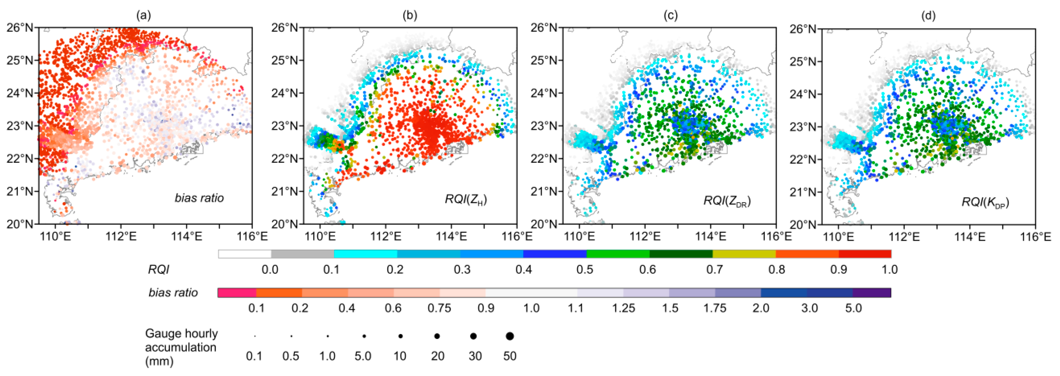
  • There is good correlation between QPE accuracy and the RQI of ZH (ZDR and KDP). An effective QPE area can be defined with an RQI of ZH lager than 0.9, resulting in a small bias (NB = −2.84%) for rainfall events in this study.
This study has presented the advantages of our proposed polarimetric radar mosaic QPE algorithm; however, only two polarimetric radars have been considered because of the limitations of data collection. In fact, since more polarimetric radars data being mosaicked together would have the benefit of more high-quality data, they would be able to obtain better QPE products. Moreover, RQI can also represent the polarimetric radar data quality, meaning this new polarimetric radar mosaic QPE algorithm can be applied to polarimetric radars of different quality. It has great potential applications to operational work; therefore, our new algorithm is expected to be used to evaluate the operational performances of more operational polarimetric radars in future studies. Although the algorithm presented here is designed for polarimetric radars in China, it may also serve as a reference for polarimetric radar mosaicking in other countries.

Author Contributions

Conceptualization, Y.Z. and L.L.; methodology, Y.Z. and L.L.; software, Y.Z.; validation, Y.Z., L.L., and H.W.; formal analysis, L.L.; investigation, Y.Z.; resources, H.W.; data curation, H.W.; writing—original draft preparation, Y.Z.; writing—review and editing, Y.Z., L.L., and H.W.; visualization, Y.Z.; supervision, L.L.; project administration, Y.Z.; funding acquisition, Y.Z. and L.L. All authors have read and agreed to the published version of the manuscript.

Funding

This research was jointly funded by the National Natural Science Foundation of China (41875036), Basic Research Fund of CAMS (2020Y017), and Scientific Research Projects of CAMS (2019Z002).

Conflicts of Interest

The authors declare no conflict of interest.

References

  1. Bringi, V.N.; Chandrasekar, V. Polarimetric Doppler Weather Radar: Principles and Applications; Cambridge University Press: Cambridge, UK, 2001; ISBN 1139429469. [Google Scholar]
  2. Chen, H.; Chandrasekar, V.; Tan, H.; Cifelli, R. Rainfall estimation from ground radar and TRMM Precipitation Radar using hybrid deep neural networks. Geophys. Res. Lett. 2019, 46, 10669–10678. [Google Scholar] [CrossRef]
  3. Zhang, J.; Tang, L.; Cocks, S.; Zhang, P.; Ryzhkov, A.; Howard, K.; Langston, C.; Kaney, B. A Dual-polarization Radar Synthetic QPE for Operations. J. Hydrometeorol. 2020. [Google Scholar] [CrossRef] [Green Version]
  4. Wen, Y.; Kirstetter, P.; Hong, Y.; Gourley, J.J.; Xue, X. Evaluation of a method to enhance real-time, ground radar-based rainfall estimates using climatological profiles of reflectivity from space. J. Hydrometeorol. 2016, 17, 761–775. [Google Scholar] [CrossRef]
  5. Zhang, J.; Howard, K.; Gourley, J.J. Constructing Three-Dimensional Multiple-Radar Reflectivity Mosaics: Examples of Convective Storms and Stratiform Rain Echoes. J. Atmos. Ocean. Technol. 2005, 22, 30–42. [Google Scholar] [CrossRef]
  6. Zhang, J.; Howard, K.; Langston, C.; Vasiloff, S.; Kaney, B.; Arthur, A.; Cooten, S.V.; Kelleher, K.; Kitzmiller, D.; Ding, F.; et al. National mosaic and multi-sensor QPE (NMQ) system: Description, results, and future plans. Bull. Am. Meteorol. Soc. 2011, 92, 1321–1338. [Google Scholar] [CrossRef] [Green Version]
  7. Xiao, Y.; Liu, L.; Yang, H. Technique for generating hybrid reflectivity field based on 3D mosaicked reflectivity of weather radar network. Act. Meteor. Sin. 2008, 66, 470–473. (In Chinese) [Google Scholar] [CrossRef]
  8. Gao, X.; Liang, J.; Li, C. Radar quantitative precipitation estimation techniques and effect evaluation. J. Trop. Meteor. 2012, 28, 77–88. (In Chinese) [Google Scholar] [CrossRef]
  9. Gou, Y.; Liu, L.; Yang, J.; Wu, C. Operational application and evaluation of the quantitative precipitation estimates algorithm based on the multi–radar mosaic. Act. Meteor. Sin. 2014, 72, 731–748. (In Chinese) [Google Scholar] [CrossRef]
  10. Chu, Z.; Ma, Y.; Zhang, G.; Wang, Z.; Han, J.; Kou, L.; Li, N. Mitigating Spatial Discontinuity of Multi-Radar QPE Based on GPM/KuPR. Hydrology 2018, 5, 48. [Google Scholar] [CrossRef] [Green Version]
  11. Zhang, J.; Howard, K.; Langston, C.; Kaney, B.; Qi, Y.; Tang, L.; Grams, H.; Wang, Y.; Cocks, S.; Martinaitis, S.; et al. Multi-Radar Multi-Sensor (MRMS) Quantitative Precipitation Estimation: Initial Operating Capabilities. Bull. Am. Meteorol. Soc. 2016, 97, 621–638. [Google Scholar] [CrossRef]
  12. Zhang, Y.; Liu, L.; Wen, H.; Wu, C.; Zhang, Y.H. Evaluation of the Polarimetric-Radar Quantitative Precipitation Estimates of an Extremely Heavy Rainfall Event and Nine Common Rainfall Events in Guangzhou. Atmosphere 2018, 9, 330. [Google Scholar] [CrossRef] [Green Version]
  13. Wang, Y.T.; Chandrasekar, V. Algorithm for estimation of the specific differential phase. J. Atmos. Ocean. Technol. 2009, 26, 2565–2578. [Google Scholar] [CrossRef]
  14. Grazioli, J.; Schneebeli, M.; Berne, A. Accuracy of phase-based algorithms for the estimation of the specific differential phase shift using simulated polarimetric weather radar data. IEEE Geosci. Remote Sens. Lett. 2013, 11, 763–767. [Google Scholar] [CrossRef]
  15. Huang, H.; Zhang, G.; Zhao, K.; Giangrande, S.E. A hybrid method to estimate specific differential phase and rainfall with linear programming and physics constraints. IEEE Trans. Geosci. Remote Sens. 2016, 55, 96–111. [Google Scholar] [CrossRef]
  16. Wu, C.; Liu, L.; Wei, M.; Xi, B.; Yu, M. Statistics–based optimization of the polarimetric radar Hydrometeor Classification Algorithm and its application for a squall line in South China. Adv. Atmos. Sci. 2018, 35, 296–316. [Google Scholar] [CrossRef]
  17. Ryde, J.W. The Attenuation and Radar Echoes Produced at Centimeter Wavelengths by Various Meteorological Phenomena. In Meteorological Factors in Radio Wave Propagation, London, U.K.; The Physical Society: London, UK, 1946; pp. 169–188. [Google Scholar]
  18. Austin, P.M.; Bemis, A.C. A Quantitative Study of the `Bright Band’ in Radar Precipitation Echoes. J. Atmos. Sci. 1950, 7, 145–151. [Google Scholar] [CrossRef] [Green Version]
  19. Wexler, R.; Atlas, D.; Mason, B.J. Factors influencing radar-echo intensities in the melting layer. Q. J. R. Meteorol. Soc. 1956, 82, 349–351. [Google Scholar] [CrossRef]
  20. Lhermitte, R.M.; Atlas, D. Doppler fall speed and particle growth in stratiform precipitation. In Proceedings of the 10th Conference on Radar Meteorology, Washington, DC, USA, 22–25 April 1963; American Meteorological Society: Washington, DC, USA, 1963; pp. 297–302. [Google Scholar]
  21. Zhang, J.; Langston, C.; Howard, K. Brightband Identification Based on Vertical Profiles of Reflectivity from the WSR-88D. J. Atmos. Ocean. Technol. 2008, 25, 1859–1872. [Google Scholar] [CrossRef]
  22. Gourley, J.J.; Calvert, C.M. Automated Detection of the Bright Band Using WSR-88D Data. Wea. Forecast. 2003, 18, 585–599. [Google Scholar] [CrossRef]
  23. Zhang, J.; Qi, Y. A Real-Time Algorithm for the Correction of Brightband Effects in Radar-Derived QPE. J. Hydrometeorol. 2010, 11, 1157–1171. [Google Scholar] [CrossRef]
  24. Qi, Y.; Zhang, J. Correction of Radar QPE Errors Associated with Low and Partially Observed Brightband Layers. J. Hydrometeorol. 2013, 14, 1933–1943. [Google Scholar] [CrossRef]
  25. Rico-Ramirez, M.A.; Cluckie, I.D.; Han, D. Correction of the bright band using dual-polarisation radar. Atmos. Sci. Lett. 2005, 6, 40–46. [Google Scholar] [CrossRef]
  26. Reino, K.; Laura, C.A.; Jason, S. Estimation of Melting Layer Altitudes from Dual- Polarization Weather Radar Observations. In Proceedings of the Eighth European Conference on Radar in Meteorology and Hydrology, Garmisch-Partenkirchen, Germany, 1–5 September 2014. [Google Scholar]
  27. Mario, M.; Nicoletta, R.; Elisa, A.; Eugenio, G.; Luca, B. Investigation of weather radar quantitative precipitation estimation methodologies in complex orography. Atmosphere 2017, 8, 34. [Google Scholar] [CrossRef] [Green Version]
  28. Friedrich, K.; Hagen, M.; Einfalt, T. A Quality Control Concept for Radar Reflectivity, Polarimetric Parameters, and Doppler Velocity. J. Atmos. Ocean. Technol. 2006, 23, 865–887. [Google Scholar] [CrossRef] [Green Version]
  29. Vulpiani, G.; Montopoli, M.; Passeri, L.D.; Gioia, A.G.; Giordano, P.; Marzano, F.S. On the Use of Dual-Polarized C-Band Radar for Operational Rainfall Retrieval in Mountainous Areas. J. Appl. Meteor. Climatol. 2012, 51, 405–425. [Google Scholar] [CrossRef]
  30. Tabary, P. The New French Operational Radar Rainfall Product. Part I: Methodology. Wea. Forecast. 2010, 22, 393–408. [Google Scholar] [CrossRef]
  31. Qi, Y.; Zhang, J. A Physically Based Two-Dimensional Seamless Reflectivity Mosaic for Radar QPE in the MRMS System. J. Hydrometeorol. 2017, 18, 1327–1340. [Google Scholar] [CrossRef]
  32. Chen, C.; Hu, Z.; Hu, S.; Zhang, Y. Preliminary analysis of data quality of Guangzhou S-band polarimetric weather radar. J. Trop. Meteor. 2018, 34, 59–67. (In Chinese) [Google Scholar]
  33. Bech, J.; Codina, B.; Lorente, J.; Bebbington, D. The sensitivity of single polarization weather radar beam blockage correction to variability in the vertical refractivity gradient. J. Atmos. Ocean. Technol. 2003, 20, 845–855. [Google Scholar] [CrossRef] [Green Version]
  34. Wen, H.; Zhang, L.; Liang, H.; Zhang, Y. Radial interference echo identification algorithm based on fuzzy logic for weather radar. Act. Meteor. Sin. 2020, 78, 116–127. (In Chinese) [Google Scholar] [CrossRef]
  35. Shi, Z.; Wei, F.; Chandrasekar, V. Radar-based quantitative precipitation estimation for the identification of debris flow occurrence over earthquake-affected regions in Sichuan, China. Nat. Hazards Earth Syst. Sci. 2017, 18, 765–780. [Google Scholar] [CrossRef] [Green Version]
  36. Qi, Y.; Zhang, J.; Zhang, P.; Cao, Q. VPR correction of bright band effects in radar QPEs using polarimetric radar observations. J. Geophys. Res. 2013, 118, 3627–3633. [Google Scholar] [CrossRef]
  37. Zhang, J.; Qi, Y.; Langston, C.; Kaney, B. Radar Quality Index (RQI)—A combined measure for beam blockage and VPR effects in a national network. In Proceedings of the Symposium Weather Radar and Hydrology, Exeter, UK, 18–21 April 2011. [Google Scholar]
  38. Wu, C. Data Quality Analysis, Hydrometeor Classification and Mosaic Application of Polarimetric Radars in China. Ph.D. Thesis, Nanjing University of Information Science and Technology, Nanjing, China, 2018. [Google Scholar]
  39. Chen, S.; Gourley, J.J.; Hong, Y.; Kirstetter, P.E.; Zhang, J.; Howard, K.; Flaming, Z.L.; Hu, J.; Qi, Y. Evaluation and uncertainty estimation of NOAA/NSSL next-generation National Mosaic QPE (Q2) over the continental United States. J. Hydrometeor. 2013, 14, 1308–1322. [Google Scholar] [CrossRef] [Green Version]
Figure 1. Distributions of the Guangzhou and Yangjiang S-band polarimetric radar (GZ SPOL, and YJ SPOL, black triangles) in (a,b), and the gauge stations (gray circles) in (b). The background color in (a) indicates altitude, and the black circles (460-km radius) indicate the maximum range of radar observations. The gauge stations are less than 300 km from either radar in (b). The gray rectangle in the lower right of (b) shows the extent of the region in South China.
Remotesensing 12 03557 g001
Figure 2. Beam blockages at 0.5° tilt of (a) Guangzhou radar and (b) Yangjiang radar. The triangles indicate radars and the narrow black area between the two radars indicates the common area for comparing data. The blockages are topped at the elevation angles of Guangzhou radar and Yangjiang radar which are shown in (c,d), respectively.
Remotesensing 12 03557 g002
Figure 3. Frequency distributions of (a) ZH, (b) ZDR, and (c) KDP from 2 km CAPPI. The horizontal axis indicates Guangzhou radar data and the vertical axis indicates Yangjiang radar data.
Remotesensing 12 03557 g003
Figure 4. Apparent vertical profile of data (AVPD) frequency distributions of (a) ZH, (b) ZDR, (c) KDP, and (d) ρHV derived from the nine rainfall events during May to June 2016.
Remotesensing 12 03557 g004
Figure 5. The ideal AVPD model of ZH, ZDR, and KDP. ht indicates the bright band (BB) top height, hb indicates the BB bottom height, hp indicates the BB peak height, and h0c indicates the 0 °C height. α and β indicate the respective slopes of the two lines.
Remotesensing 12 03557 g005
Figure 6. The models of (a) RQIblk, (b) RQIhgt, (c) RQIsnr, and (d) RQIΡHV. hb in (b) is the height of the BB bottom. Lines 1, 2, and 3 correspond to Hsf values of 500 m, 1500 m, and 2500 m, respectively. The SNR * s (corresponding to snr * s) of the dotted and solid lines in (c) are 0 dB and 25 dB, respectively.
Remotesensing 12 03557 g006
Figure 7. Flowchart describing the polarimetric radar data mosaic algorithm. The “data points” are original resolution polar data of different radars corresponding to the same ground grid.
Remotesensing 12 03557 g007
Figure 8. Flowchart describing the quantitative precipitation estimation (QPE) algorithm.
Remotesensing 12 03557 g008
Figure 9. ND frequencies of (a) ZH, (b) ZDR, and (c) KDP are shown with histograms. The gray ones are derived from corrected data, and those with black lines outside are derived from raw data in the BB.
Remotesensing 12 03557 g009
Figure 10. The original mosaics for (a) ZH, (b) ZDR, (c) KDP, and (d) ρHV at 20:54 UTC on 15 June, 2016. The corrected mosaics for (e) ZH, (f) ZDR, and (g) KDP are also shown, respectively. The mosaic data are from the lowest hybrid scans in original polar coordinates. The colors in (h) represent BBA (blue) and non-BBA (gray). The triangles indicate radars. The black circles in (ah) indicate the main areas that are affected by BB. The AVPDs of (i) ZH, (j) ZDR, (k) KDP, and (l) ρHV, as derived from Guangzhou radar, are also shown. Black dots indicate the original observations, and red dots indicate the corrected values. The corresponding feature heights are marked in the figures.
Remotesensing 12 03557 g010
Figure 11. The ideal mosaic height. Three areas marked by boxes. Regions 1, 2, and 3 are mainly located at 3–5 km height, and are easily affected by BB.
Remotesensing 12 03557 g011
Figure 12. Mosaics for (a) ZH, (b) ZDR, (c) KDP, (g) ρHV, and (i) SNR at 5:00 UTC on 20 May 2016. The corresponding RQIs of (d) ZH, (e) ZDR, (f) KDP, and (h) ρHV are also shown next to the radar data. The triangles indicate radars.
Remotesensing 12 03557 g012
Figure 13. Bias ratio distributions of (a) radar mosaic QPE and (b,c) two single radars’ QPEs. A gauge corresponds to a bias ratio value. The bias ratio is computed with the pairs of radar-estimated precipitation and gauge-observed precipitation of this gauge. The evaluation area is less than 300 km from the two radars, and the evaluation results are based on all nine rainfall events. Bubbles indicate the bias ratio at the gauge stations. Different colors indicate different bias ratio values. Red indicates underestimation and purple indicates overestimation. Bubble size indicates the average hourly rainfall accumulation at each gauge. The inner distance of the spindle shape marked with a black line is less than 180 km from either radar.
Remotesensing 12 03557 g013
Figure 14. (ai) Time series of RMSEs derived from the nine rainfall events. QPE is also evaluated in the area less than 180 km from either radar. Green, blue, and red lines represent RMSEs derived from Guangzhou radar QPE, Yangjiang radar QPE, and radar mosaic QPE, respectively.
Remotesensing 12 03557 g014
Figure 15. Bias ratio distributions of the QPEs estimated by the algorithm without (a) and with (c) BB correction. The color bubbles are the same as those in Figure 13. The associated scatterplots of the QPEs before (b) and after (d) improvements vs. gauge data in regions 1, 2, and 3 are also shown.
Remotesensing 12 03557 g015
Figure 16. (a) RMSEs, (b) NEs, and (c) NBs changing with the percentage of convective precipitation. The precipitation in these tests is only mixed with convective precipitation and stratiform precipitation. The percentages of stratiform precipitation are from 100% to 0% from left to right.
Remotesensing 12 03557 g016
Figure 17. AVPDs of (ac) ZH and (df) ZDR. Black dots indicate the original observations and red dots indicate the corrected values. Green lines represent the changing trends of the ZH and ZDR profiles under BB. The corresponding times and feature heights are marked in the figures. “GZ” means data are derived from the Guangzhou radar, and “YJ” means data are derived from the Yangjiang radar.
Remotesensing 12 03557 g017
Figure 18. (a) Bias ratio distribution of the radar mosaic QPE within almost the entire range that can be detected by the two radars. The color bubbles in (a) are the same as those in Figure 13. (bd) present the area distributions of the average RQI of ZH, ZDR, and KDP, as derived from nine rainfall events. The color bubbles in (bd) indicate the average values of RQI at the gauge stations. Different colors indicate different RQI values. The bubble size indicates the average hourly rainfall accumulation at each gauge.
Remotesensing 12 03557 g018
Table 1. Main specifications of the S-band polarimetric radar.
Parameter TypeSetting
The antenna diameter (m)8.54
The antenna gain (dB)45.31
The beam width (°)<0.98
The first side lobe (dB)<−30
The wave length (cm)10.3
The operating modesimultaneous horizontal and
vertical transmission and reception
The minimum detectable power (dBm)−117.8
The volume scan modeVCP21 (9 tilts)
The range resolution (km)0.25
Table 2. A list of the nine rainfall events used in this study.
#Date (UTC)Total Time (h)No. of Valued GaugesMean Gauge Accumulation (mm)Max Gauge Accumulation (mm)Precipitation Type
16 May 20161273019.04118.5squall line
29–10 May 20163490534.68222.8convective
315 May 20161096314.1967.1squall line
419–21 May 201643100155.77416.6stratocumulus
527–28 May 20162499130.48177.2squall line
64–5 June 20162493529.20109.4stratocumulus
79 June 201682699.5680.2stratocumulus
811–14 June 201686100744.57211.4stratocumulus
915 June 2016671911.9979squall line
Table 3. Evaluated statistical scores of radar QPE based on raw/corrected data in the BB. Radar QPE based on data at the BB bottom height is treated as the “truth” value.
MethodBased on Raw Data in BBBased on Corrected Data in BB
CCNE (%)NB (%)CCNE (%)NB (%)
R1(ZH)0.3941.6637.550.8011.79−1.24
R2(ZH)0.3940.4236.420.8011.50−1.22
R1(KDP)0.15100.273.300.2660.2816.96
R2(KDP)0.1597.5271.140.2659.0216.41
R(ZH,ZDR)0.5238.3831.060.8713.811.53
R(KDP,ZDR)0.1693.3966.610.2659.3016.17
Table 4. Evaluated statistical scores of radar mosaic QPE, as well as those of the two single radars.
MethodCCRMSE (mm)NE (%)NB (%)
Radar mosaic QPE0.863.7639.72−5.89
Guangzhou Radar QPE0.853.9742.07−2.06
Yangjiang Radar QPE0.655.8864.26−29.30
Publisher’s Note: MDPI stays neutral with regard to jurisdictional claims in published maps and institutional affiliations.

