Abstract
The Surface Water and Ocean Topography (SWOT) satellite mission, expected to launch in 2022, will enable near global river discharge estimation from surface water extents and elevations. However, SWOT’s orbit specifications provide non-uniform space–time sampling. Previous studies have demonstrated that SWOT’s unique spatiotemporal sampling has a minimal impact on derived discharge frequency distributions, baseflow magnitudes, and annual discharge characteristics. In this study, we aim to extend the analysis of SWOT’s added value in the context of hydrologic model calibration. We calibrate a hydrologic model using previously derived synthetic SWOT discharges across 39 gauges in the Ohio River Basin. Three discharge timeseries are used for calibration: daily observations, SWOT temporally sampled, and SWOT temporally sampled including estimated uncertainty. Using 10,000 model iterations to explore predefined parameter ranges, each discharge timeseries results in similar optimal model parameters. We find that the annual mean and peak flow values at each gauge location from the optimal parameter sets derived from each discharge timeseries differ by less than 10% percent on average. Our findings suggest that hydrologic models calibrated using discharges derived from SWOT’s non-uniform space–time sampling are likely to achieve results similar to those based on calibrating with in situ daily observations.
Keywords:
hydrologic modeling; calibration; discharge; SWOT; remote sensing; spatiotemporal sampling 1. Introduction
Hydrologic and hydrodynamic models are useful for assessing climate change impacts [1], predicting flood characteristics, forecasting applications [2], and understanding the transfer and storage of water and energy globally [3]. Satellite remote sensing has been utilized to quantify and assess water security [4], and measurements can be coupled with hydrologic models to improve overall discharge estimation [5,6,7,8,9]. In many modeling applications, calibration methods are used to optimize model parameters for estimating river discharge [10,11,12,13,14]. These techniques, data assimilation and calibration, are valuable tools used in efforts focused on understanding river discharge dynamics.
The upcoming Surface Water and Ocean Topography (SWOT) satellite mission will enable discharge estimation at an unprecedented global scale using wide swath interferometry measurements of surface water extents and elevations that are uniquely distributed through space and time. Jointly developed by the National Aeronautics and Space Administration (NASA) and the Centre National d’Etudes Spatiales (CNES) with participation from the Canadian and UK space agencies, SWOT will observe oceans, lakes/reservoirs, rivers, estuaries, seas, and land ice. For this paper, we will focus on hydrologic modeling applications, namely applications of SWOT measurements relating to rivers. SWOT will observe river surface height, width, and slope for at least 90% of rivers wider than 50–100 m [15]. These measurements can be used in SWOT flow inversion algorithms to estimate discharge [16,17]. Expected to launch in 2022 at the time of this writing, the satellite will utilize a 21-day repeat orbit cycle within ±78 degrees latitude, observing the latitude near the poles more often than near the equator per cycle [15]. SWOT observations will be unevenly distributed in space/time throughout the 21-day cycle [18]. For example, if a location is measured three times in the orbit cycle, this does not indicate it will be measured every seven days (i.e., the observations could be on days 8, 19, and 20). In addition, locations near each other may not be observed an equal number of times. Ref. [19] shows that in the Mississippi River Basin, locations vary in being observed from zero to four times during the orbit cycle.
Previous studies suggest that discharges derived from the SWOT satellite’s irregular temporal and spatial sampling can be used in numerous hydrologic applications. For example, discharge frequency distributions are often used in the hydrology community to calculate storm return periods and estimate flood hazards. Ref. [19] finds that the unique temporal sampling of SWOT has no significant impact on derived frequency distributions at 442 US Geological Survey (USGS) streamflow gauge sites in the Mississippi River Basin. When uncertainty is also included based on specific SWOT discharge algorithm performance error metrics, no statistical difference is still observed in 78% of gauge site distributions. Identifying river baseflow levels is another important application that helps evaluate the impact of climatic and anthropogenic stresses on the availability of water resources, and [20] finds that the SWOT mission will be able to effectively measure baseflow despite its irregular sampling. Flow duration curves are used in applications regarding water management and supply for human and irrigation purposes. Their derivation using synthetic SWOT data gives reliable estimation of the Po River flow regime despite the unique sampling [6]. Measuring reservoir storage change using SWOT, Ref. [21] finds temporal sampling would not cause severe aliasing in 87% of sites when converting reservoir water storage data to monthly values, although they test at regular intervals depending on the amount of days the reservoir would be observed in the 21-day orbit cycle. Ref. [22] concludes that SWOT will augment our ability to detect and size floods by simultaneously measuring water surface elevation and inundation extents, which is an unprecedented feat on this scale, although SWOT would have observed only 55% of 4664 floods in their study database.
In this study, we extend the analysis on the potential value of SWOT discharge products in the context of hydrologic model calibration, specifically considering SWOT’s unique spatiotemporal sampling and discharge uncertainty. Spatial altimetry data [23] and satellite imagery [24] have historically been integrated into calibrating hydrologic models. Previous studies have explored calibration in the context of SWOT-like observations. Ref. [9] discusses how SWOT-like data could be used to optimize large-scale hydrologic model parameters with data assimilation techniques. Ref. [25] investigates the potential of SWOT to correct hydrologic models on a global scale through data assimilation, finding model discharge errors reduced by 40%. Ref. [26] calibrates a hydrologic model using daily continuous river discharge estimated from SWOT-like observations in ungauged basins, retrieving Nash–Sutcliffe efficiency values as high as 0.85. In their study, they used Landsat-derived river widths and concurrent in situ water levels to produce synthetic SWOT observations. Landsat has a repeat orbit of approximately 16 days, and water level was obtained daily. Although these studies present a more accurate representation of SWOT-like measurements, they do not test whether the specific sampling frequency of SWOT due to orbit limitations would be useful in the context of hydrologic model calibration. Our central research question is: Does model performance change significantly if calibrated using synthetic, temporally irregular SWOT-derived discharges rather than using daily discharges? We opt for a more focused approach, purely studying whether synthetic SWOT timeseries will be useful in the context of hydrologic model calibration without utilizing data assimilation.
We calibrate surface and subsurface runoff generated based on the Variable Infiltration Capacity (VIC) model equations [27], which are routed throughout the river network with the Hillslope River Routing (HRR) model [3]. We use discharges from 39 gauges in the Ohio River Basin for the 9-year period 2010–2018. Three different discharge timeseries are used for calibration: daily USGS gauge observations, SWOT temporally sampled, and SWOT temporally sampled including estimated uncertainty expected from SWOT measurements. To calibrate the coupled models, 10,000 model iterations are simulated, where four VIC runoff parameters are systematically altered within predefined ranges. The calibrated parameter set is selected from the model iteration providing the best performance based on the discharge timeseries being considered. Relationships between calibration parameters are discussed, selected parameter sets are compared, and results are tested for sensitivity using different 3-year calibration periods rather than the full 9-year period, emulating possible mission lifetimes. The goal of this study is to ascertain whether calibration using a synthetic SWOT-derived discharge timeseries instead of daily measurements would change model performance significantly.
2. Materials and Methods
2.1. Data Used to Simulate SWOT Mission Discharge
The study region is comprised of the SWOT observable river network in the Ohio River Basin, USA (Figure 1). The basin has a drainage area of 525,300 km2, and the rivers incorporated in the study are from the Global River Widths from Landsat (GRWL) Database [28]. At mean flow conditions averaged over 10 km reaches, GRWL rivers have widths of 90 m or wider. Since SWOT measurements will enable discharge products for rivers exceeding 50–100 m wide [15], we selected the GRWL database as a good approximation of SWOT observable rivers. GRWL rivers are used to determine which gauges would be observed by SWOT; the hydrologic model does not use the associated river widths from the dataset.
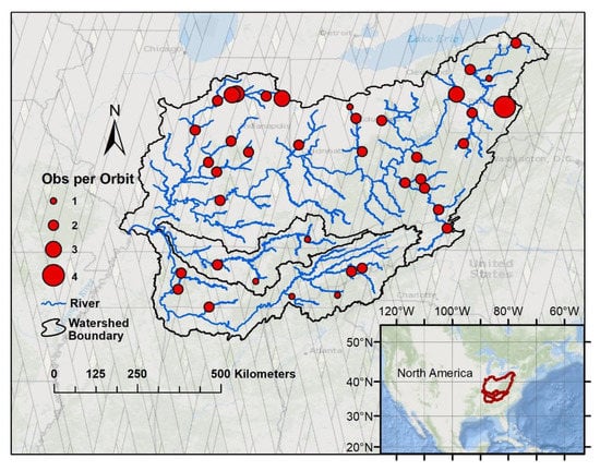
Figure 1.
The 39 US Geological Survey (USGS) gauges used for calibration in the Ohio River basin, a 525,300 km2 watershed, showing streams greater than 90 m wide and Surface Water and Ocean Topography (SWOT) swaths. The differing gauge sizes indicate the number of days SWOT will obtain measurements at each site per 21-day orbit cycle.
For the study, 39 USGS streamflow gauges, with daily data available for the 9-year period from 1 January 2010 to 31 December 2018 located along the GRWL rivers were selected. Gauges were strategically selected so that the correlation coefficient between any two gauges does not exceed 0.9. This was done so that one section of the river does not dominate the calibration process, as gauges near each other tend to have highly correlated discharge. Figure 1 shows the specific gauge locations on the river network along with the number of observations each gauge will have within the 21-day orbit cycle, with a possible range of observations in this basin being from zero to four times. Most gauges selected will be observed twice in the orbit cycle. Each pass of the satellite consists of two 50 km swaths with 20 km between each swath, as pictured in Figure 1 [29].
For calibration, three different discharge timeseries were used: gauge discharge (Qg), SWOT temporal discharge (Qgs), and synthetic SWOT discharge (Qs). Qg was downloaded from USGS for the 39 gauges shown in Figure 1 on a daily timescale; a list of the gauges can be found in the supplemental materials (Table S1). Qgs is a subset of Qg discharge timeseries that only contains measurements for days SWOT would pass over each gauge site in the 21-day orbit cycle, assuming an initial orbit cycle starts on 1 January 2010. The subset of data for Qgs was determined by spatially joining a SWOT orbit shapefile and the desired USGS gauge points to find what days SWOT would gather observations at each site. The distinction and process of deriving the Qs timeseries as synthetic SWOT data is also described fully in [19], but we present a summarized version here. Qs follows the same temporal pattern as Qgs, but with the addition of uncertainty considering the potential relative bias (rBIAS) and relative root-mean-square-error (RRMSE) associated with [17]’s SWOT discharge algorithm, the Bayesian At-many-stations Hydraulic Geometry (AMHG)-Manning (BAM) algorithm. By studying potential SWOT errors from 19 study rivers, they found that the median RRMSE is 42% and the median rBIAS is –17%. RRMSE is more representative of the spread or standard deviation of the data, while rBIAS indicates a tendency of the timeseries toward over or underestimation. In this instance, [17] reports a tendency toward underestimation of –17%. To include uncertainty in deriving Qs, we transform these performance metrics into the log-space and use them to estimate a log mean and standard deviation for a random Gaussian error distribution. Each SWOT sampled discharge value is transformed into the log-space, uncertainty from the lognormal Gaussian distribution is added, and the value is transformed back from the log-space, akin to [19]. The log-space is utilized so that associated uncertainty over both small and large discharge measurements give representative magnitudes of error. It is important to note that the uncertainty for Qs is highly dependent on the selected discharge algorithm, BAM.
2.2. HRR-VIC Model and Input Data
The hydrologic model used is a modified version of the Hillslope River Routing (HRR) model [1,3], which now derives surface and subsurface flow using the Variable Infiltration Capacity (VIC) model formulation equations [27]; it is termed the HRR-VIC model. HRR is a topography-based routing model that integrates surface and subsurface runoff laterally into river channels and routes discharges throughout the river network based on the Muskingum–Cunge method, resulting in discharge estimates for each river reach. Each model unit consists of a river reach and its associated catchment boundaries that become approximated by two planes draining laterally into the main river channel. This effort builds on previous studies that coupled the HRR and VIC models to estimate streamflow [1,30]. The resulting modeled discharge estimates from HRR-VIC will be referred to as Qm.
This specific river network used for the HRR-VIC model in the Ohio River Basin is discretized into 237 model units with a single discharge value assigned per model unit [3]. The average drainage area associated with each model unit is roughly 2200 km2, which is on order with the minimum drainage area associated with rivers having widths 50–100 m or larger (i.e., observable with SWOT) [18]. HRR-VIC operates on an hourly temporal resolution, with river discharges averaged to daily for comparison to the reference discharges series. Each model unit also contains its own set of soil properties based on the Global Soil Dataset for use in Earth System Models (GSDE) [31]. Forcings data were obtained for the period 1 January 2010 through 31 December 2018: a total of nine years. NASA’s North American Land Data Assimilation System (NLDAS) primary forcings—hourly precipitation, potential evaporation, and 2-m above ground temperature products [32,33]—were used to force the hydrologic model. NLDAS potential evaporation directly considers land cover and vegetation in its derivation, and thus, HRR-VIC does not utilize additional land cover estimates. All input data were spatially averaged over each model unit.
The HRR model originally did not account for snowmelt, and since snow accumulation is a factor in the Ohio River Basin, albeit a small component [34], we decided to incorporate a simple snowmelt model into the derivation of surface and subsurface flow. We have modified the HRR-VIC model to account for snowmelt following the United States Department of Agriculture (USDA)’s degree-day method [35] when snow is present and the temperature is above 1 degree Celsius [36]. The USDA gives typical melt rate values between 0.07 and 0.25 mm/°C-hr, and we select a constant value of 0.2 mm/°C-hr to represent the melt rate of snow when rain is not present. When rain is present, the melt rate is changed to 0.3 mm/°C-hr, which is about one standard deviation above the mean snow melt value reported in [37]. Although it is a simplified snowmelt modeling approach, the degree-day method has been demonstrated to accurately simulate snow accumulation and melt, and when coupled with a hydrologic model, it gives similar results to a more complex energy balance method [38].
Datasets, the HRR-VIC model, and all the codes used for this research are available through CUAHSI’s HydroShare (https://www.hydroshare.org/) with the following DOI: 10.4211/hs.172bf3533b1d46ea8d89feea51d44fb7 [39].
2.3. Model Calibration
2.3.1. Variables and Spatial Variation
Four VIC runoff parameters are calibrated: the variable infiltration curve parameter (bi), the upper soil layer depth (usoilD), the maximum velocity of baseflow (Dsmax), and the fraction of Dsmax where nonlinear baseflow begins (Ds) (Table 1). Akin to [14], bi, usoilD, and Ds were selected as suitable parameters for calibration with the addition of Dsmax according to previous sensitivity analyses with VIC model parameters [10,11,13]. Although we only calibrate four parameters, these parameters alone alter model behavior significantly. The focus of this manuscript is not how to best optimize the HRR-VIC model, but rather to analyze how or if model results (Qm) change when calibrating using the different timeseries (Qg, Qgs, and Qs). Ten values of each parameter are selected for calibration, starting at the lowest value in the range and increasing in value by the “step” indicated in Table 1 until the maximum value of the range. With four variables of ten values each, all permutations result in 10,000 iterations (104). It is to be noted that for our purposes, parameter value options have been limited to produce a more systematic experimentation rather than 10,000 random iterations. Other studies often test bi from 0.001 to 0.8, usoilD from 0.1 to 2.0 m, Dsmax from 0 to 40 mm/d, and Ds from 0.01 to 1.0 [10,11,12,13,14]. Our parameter value selections align with these values, even bi, which we have spatially varied so that when the median bi = 0.4, some locations have bi = 0.8, as explained below. As a result of the method we have selected, increasing by steps of values, it is indeed possible that more optimal parameter sets would exist within these ranges. However, having pre-determined possible values rather than random iterations facilitates ease of comparison among calibration results of the differing timeseries.

Table 1.
Variable Infiltration Capacity (VIC) parameter explanations and their ranges used for calibration.
The variable infiltration curve parameter (bi) controls the shape of the effective soil moisture capacity distribution over a region and essentially dictates the partitioning of rainfall into surface runoff versus infiltration. A smaller value of bi increases the infiltration capacity, therefore decreasing surface runoff [10]. It is difficult to estimate bi directly from field measurements, and therefore, it is usually determined through model calibration [11]. For this study, bi is spatially varied, which is explained in detail below. The range given in Table 1 indicates the range of the median bi value, while individual locations could have bi values double and half the median.
Unlike bi, the other calibrated parameters are without spatial variation in the model. The upper soil layer depth (usoilD) is referred to as thick2 in previous literature, but to remain consistent with current HRR model variables, we have used the term usoilD. Although the VIC model can have more soil layers, the HRR-VIC model uses two soil layers: the upper soil layer and lower soil layer. From previous studies using VIC model parameters for calibration, it was found that the upper soil layer was by far the most sensitive [10]. Therefore, the lower soil depth is held constant at 1 m. Thicker soil depths have the capability to retain more water and therefore decrease the surface runoff and increase the loss due to evapotranspiration [14]. The maximum velocity of baseflow (Dsmax) is a numerical value that can be measured, but it also can be calibrated. A larger Dsmax increases the amount of subsurface runoff entering the channel within an allotted time frame. Ds is a more theoretical parameter that controls the baseflow rate. It typically has a high positive correlation with Dsmax because Ds represents the fraction of Dsmax at which nonlinear baseflow begins [13].
Our network of rivers in the Ohio River Basin is discretized into 237 model units with a single discharge value assigned per model unit [3]. Each model unit has a saturated hydraulic conductivity (Ksat) value associated with it from [31] used for calculations (Figure 2). The larger the Ksat value, the more infiltration occurs. The smaller VIC’s bi value, the larger the infiltration [10]. Thus, we varied bi with a multiplier (0.5, 0.75, 1.0, 1.5, or 2.0) based on ranges of the Ksat value spatially seen in Figure 2. The bi value that we change is the median bi value, with the maximum spatial bi value being double the median, and the minimum being half the median. Although the variation range of the median bi is given as 0.04 to 0.4, considering the spatial variation, bi values can be between 0.02 and 0.8. The Clapp and Hornberger coefficient used in the VIC equations also varies by Ksat because a measured correlation exists between the two. The Clapp and Hornberger Coefficient (cc) derived from b values (cc = 2b + 3) and its associated Ksat measurements that were reported in [40] were plotted. A power trendline was fit to the points, giving a correlation coefficient of 0.81 and implemented in the HRR-VIC model as .
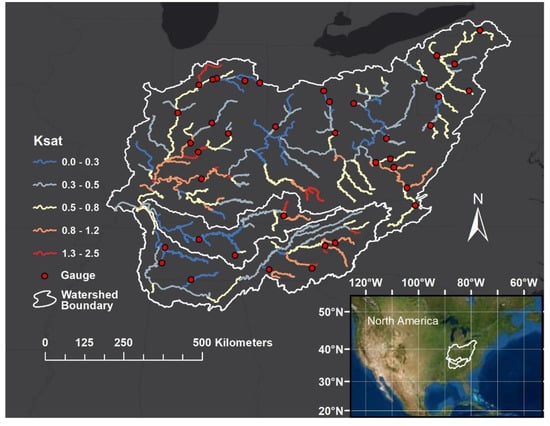
Figure 2.
The 237 model units of the Ohio River basin network colored by hydraulic conductivity (ksat) with points denoting the 39 USGS gauges used for calibration.
2.3.2. Calibration and Sensitivity Analysis
For the experiment, 10,000 model iterations are performed using permutations of 10 set values within the given testing range for each of the four VIC parameters outlined in Table 1. In each iteration, an error metric is calculated comparing the model output (Qm) to Qg, Qgs, and Qs each individually to assess which parameter set produced the best error metric per timeseries. The iteration resulting in the best error metric is deemed as the optimal or “calibrated” parameter set for the respective discharge timeseries being considered. The goal is to see if calibrating the model using the different timeseries (Qg, Qgs, or Qs) produces similar results, thus providing insights on the applicability of SWOT measurements with their irregular timeseries and uncertainty to be used in model calibration.
Since SWOT’s mission objectives are planned for completion within three years once the satellite has been launched, there is the potential that only three years of measurements will be available, although satellites are known to give measurements beyond their original mission life. With this in mind, we want to know how sensitive the calibration is to the duration of the SWOT measurements obtained. We split the nine years of data into three 3-year time periods (2010–2012, 2013–2015, and 2016–2018) to compare how calibration results change based on the selected period.
To assess the performance of each parameter set, the Kling–Gupta efficiency (KGE) [41] is calculated between model results (Qm) and each of the three timeseries (Qg, Qgs, or Qs) individually. KGE is defined as:
where r is the correlation coefficient, β is the bias ratio, and γ is the relative variability between two timeseries. In this case, Qm is the model discharge and Qo is the observed discharge, meaning one of the three timeseries (Qg, Qgs, or Qs). μ indicates the mean and σ indicates the standard deviation of the specified timeseries. A KGE of 1 indicates that the model simulated exactly what was observed. Unlike the commonly known Nash–Sutcliffe efficiency, KGE values greater than –0.41 indicate that a model improves upon the mean flow benchmark (i.e., KGE values > –0.41 are better than the mean) [42]. The best iteration was selected based on whichever produced the highest median KGE value across the 39 gauges.
3. Results
3.1. VIC Parameter Trends and Relationships
Investigating how each VIC parameter influenced median KGE values (comparing Qm vs. Qg) from the 39 gauges for all 10,000 iterations (Figure 3) highlights one parameter, usoilD, above all others as having a strong signal. As usoilD increases from 0.2 to 1.4 m, the median KGE tends to increase, and as usoilD increases from 1.4 to 2.0 m, overall, median KGE values show a decreasing trend. The range of median KGE values for each tested value of usoilD also differs drastically, with soil layer depth of 0.2 m having median KGE values ranging from –0.14 to 0.37 and a soil layer depth of 1.4 m resulting in median KGE values ranging from 0.28 to 0.51. For the lower range of soil depth values (0.2–1.0 m), when bi, Dsmax, and Ds are smaller, median KGE values tend to be highest, but as usoilD increases to 2.0 m, the best KGE values occur when bi, Dsmax, and Ds are larger. In other words, the model parameters are shifting to balance their impacts on runoff production. For example, a smaller usoilD indicates less evapotranspiration (ET) and greater runoff. Smaller bi values lead to more infiltration, supporting more ET and less runoff. Thus, to account for the higher runoff production due to smaller usoilD values, bi values must be smaller. A smaller Dsmax is indicative of a lower baseflow and therefore also decreases the amount of water delivered to the channel network. Smaller values of Ds, the fraction of Dsmax where nonlinear baseflow begins, again tends to decrease channel discharge. When the median KGE values are the greatest (usoilD = 1.2–1.4 m), these four parameters balance each other, resulting in values nearer the middle of each parameter range, emulating most accurately gauge discharge. The right side of Figure 3 shows that the other VIC parameters do not exhibit a strong signal with median KGE. The bi values show a slight increase in median KGE values at around 0.16–0.20 for the upper range of median KGE values, yet the smaller the value of bi, the less likely the iteration is to have a KGE below zero. Often for this model, surface runoff controls during events rather than baseflow, so the impact of Dsmax and Ds is not as prevalent. Although, similar to bi, the smaller the value of each Dsmax and Ds indicates a smaller likelihood of the median KGE being less than zero. All values greater than 8 mm/d for Dsmax and 0.2 for Ds do not seem to have much advantage over the others. No obvious patterns emerge in the relationships of bi with other variables, as [13] also found. Dsmax and Ds do not seem to have a correlation with each other in relation to median KGE values, either. We acknowledge that because we are setting Dsmax and Ds as constant through the whole Ohio River basin network, we are not able to effectively test the correlation between parameters as other studies with spatial gridded optimal values have done [13].
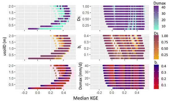
Figure 3.
Relationships between the four VIC parameters calibrated (bi, usoilD, Dsmax, and Ds). Each panel shows the relationship between a specific parameter and median Kling–Gupta efficiency (KGE) value from the 39 gauges per iteration. Points are colored by a different parameter value per panel, with the legend showing the range in values. For instance, the left three panels have the same base graph, plotting usoilD vs. median KGE, but they are colored by Dsmax, Ds, and bi ranges, respectively. The model is calibrated using gauge discharge (Qg) for all 10,000 iterations. bi: variable infiltration curve parameter, Dsmax: maximum velocity of baseflow, Ds: fraction of Dsmax where nonlinear baseflow begins, usoilD: upper soil layer depth.
3.2. Iteration Comparisons among Timeseries
When calibrating the model using the different discharge timeseries to obtain median KGE values, the same trends exists in all parameters, although the ranges in KGE values may differ, for example with usoilD and its relationship with bi (Figure 4). For the median KGE of the 39 gauges, Qg and Qgs have similar ranges, but Qs has markedly larger ranges of median KGE values, especially when usoilD is equal to 0.2 m (ranging from –0.38 to 0.31). Note that all median KGE values are above the –0.41 KGE threshold discussed in the methods, indicating that the model improves upon the mean flow benchmark and that individual gauges have values that are below the threshold. The maximum KGE from an individual gauge out of the 39 is also shown, and KGE values for all three timeseries (Qg, Qgs, Qs) vs. Qm are between 0.47 and 0.82. Given that the maximum KGE possible is 1.0, the modeled discharge and each timeseries have good correlation. The range of maximum KGE values is the smallest using Qg, but the best maximum KGE values were achieved in calibration using Qgs, which is not immediately intuitive. An explanation of why this may be the case can be found in the discussion.
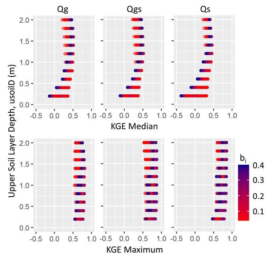
Figure 4.
Relationships between bi and usoilD using median and maximum KGE values over the 39 gauges calculated from calibration using each discharge timeseries (Qg, Qgs, Qs). Qgs: SWOT temporal discharge, Qs: synthetic SWOT discharge.
The parameter sets that produced the highest median KGE value from the 39 gauges for each timeseries comparison are shown in Table 2. The KGE performance is most reliant on usoilD, and thus intuitively, the highest median KGE values align with similar usoilD values for each comparison. Qg and Qs are both optimized with 1.4 m of upper soil layer depth, while Qgs is optimized when the depth is 1.2 m. Optimized values for Ds and Dsmax vary greatly across the timeseries. For reference, the average mean annual flow (MAF) measured at the gauge locations is 1.5 mm/d, which was found by dividing the MAF by the drainage area per site, and it is an order of magnitude smaller than Dsmax. Qg and Qs are optimized when bi is 0.16, but Qgs is optimized when it is 0.04. These three specific parameter sets give hydrologic model results, and they are referred to as Model A, B, and C for the selected top iteration of each timeseries: Qg, Qgs, and Qs, respectively.
Table 2.
Parameter values from the best iterations per timeseries (Qg, Qgs, Qs) determined by the median KGE of 39 gauges. The set letters (A, B, and C) are used to refer to the selected parameter sets further in the paper.
Example hydrographs for the gauge site, White River at Newberry, IN (USGS 03360500), illustrate each timeseries and the optimized modeled discharge over a two-month period in 2011 (Figure 5a). This gauge will be observed twice in the 21-day orbit cycle: days 5 and 17. This gauge performs well, giving KGE values greater than 0.71 over the 9-year period for all three timeseries comparisons. Figure 5b shows 2011 discharge ranked from largest to smallest for all three calibrated models. Since the modeled discharge calibrated using Qgs, model B, uses an optimal depth at 1.2 m, as opposed to 1.4 m as the others, less infiltration into the soil can occur. When the soil is at saturated capacity, more runoff is generated, and the magnitude of the model B discharge is higher. During low-flow conditions, there is less separation between modeled discharge results because less runoff occurs in general. Since both bi and usoilD’s optimized values were the same for model A and model C, which were calibrated according to the top KGE iteration of Qg and Qs, respectively, the difference in modeled hydrographs is attributed to Dsmax and Ds, which control subsurface or baseflow. The combination of Dsmax and Ds for model A results in higher baseflow values than for those of model C, which is more obviously observed in the hydrograph during peak flows.
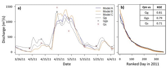
Figure 5.
For gauge 03360500, (a) example hydrographs showing each original timeseries (Qg, Qgs, Qs) and the model outputs (A, B, C) for their optimal parameter sets for each timeseries calibration, and (b) the ranked discharge from high to low of model outputs in the year 2011 are shown. Kling–Gupta efficiency (KGE) values for the entire 9-year timespan for this gauge are also given. The gray line is the daily gauge timeseries (Qg), the black xs indicate SWOT sampling discharge (Qgs), and the red xs indicate SWOT sampling with added uncertainty (Qs), as outlined in Section 2.2. There are three modeled discharge timeseries representing modeled discharge: the modeled discharge results for the top iteration when Qg is used for calibration, model A, when Qgs is used for calibration, model B, and when Qs is used for calibration, model C. Each has been obtained with the specified set of VIC parameters listed in Table 2.
To further determine whether results based on calibrating Qm with each timeseries are consistent, the top 100 iterations out of the 10,000 were also compared with each other (Figure 6). The iterations with the top 100 median KGE values are ranked according to the median KGE of Qm vs. each individual timeseries (Qg, Qgs, Qs), and thus, each iteration has three median KGE values. Figure 6 shows three different ranking orders of the top 100 iterations, although the iterations in the top 100 are not necessarily the same in all three plots. For each plot, the top 100 iterations are selected based on the greatest 100 median KGE iterations for that comparison, and the other KGE values for these iterations also shown. For example, the first plot shows the top 100 iterations as defined by ranking Qm vs. Qg’s median KGE values. These same parameter sets used to obtain the top iterations of Qm vs. Qg also obtain KGE values for Qm vs. Qgs, and Qm vs. Qs, which are displayed on the plots as well. When the top iterations are selected and shown in Qg and Qgs’s ranked order, the magnitude of their highest median KGE values do not differ greatly, with their highest values between 0.50 and 0.52. Qs’s highest median KGE values remain close to 0.46 for all its top 100 iterations. It is interesting to note that many Qs KGE values close to 0.46 appear in the iterations selected when ranking according to Qg and Qgs, yet the top 20 median KGE values for Qgs only seem to appear on the middle plot that is ranked according to Qgs. In other words, the top parameter sets selected for Qgs are not the same as the top iterations selected when ranking by Qg and Qs. The optimal parameters obtained from ranking according to Qg KGE generate the highest KGE values for all three timeseries collectively (the most left plot in Figure 6), suggesting that calibration using Qg gives more robust model parameters.
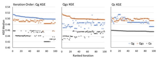
Figure 6.
The median KGE values for the top 100 iterations shown three times; each graph is ranked greatest to least in order of the median KGE value for each discharge timeseries (Qg, Qgs, Qs). Each graph has a total of 300 points, three KGE values comparing how each timeseries compared to the model (Qm) for each specific iteration.
Breaking down the top 100 iterations into histograms of the optimal parameter values selected (Figure 7) highlights similar patterns as discussed above for the best iterations recorded in Table 2. Again, calibrating using Qg, Qgs, and Qs all lead to usoilD values between 1.2 and 1.6 m, although Qg tends toward 1.6 m in the top 100 iterations, while Qgs tends toward 1.2 m and Qs is split relatively evenly between 1.2 and 1.4 m as the optimum upper soil layer depth. For bi, the mode selected when calibrating with Qg is 0.2, while Qs produces the most iterations in the top 100 with 0.12, and Qs is again split relatively evenly between 0.12 and 0.16. It is interesting to note that Qgs’s top run has a bi value of 0.04, although less than five iterations in the top 100 also have this value. bi values above 0.24 are not in the top 100 iterations for any of the timeseries. Dsmax and Ds have a wide range of values in the top 100 iterations for all three timeseries. The only value that is not represented for Dsmax is 4 mm/d. One selection is not obviously better than any others, although 12 mm/d seems to be the mode for both Qg and Qgs, while 40 mm/d is the mode for Qs. Ds has modes at 0.3 (Qg), 0.5 (Qgs), and 0.6 (Qs), although again, the spread over all the possible ranges is large. The large spread of Ds and Dsmax in the top 100 support the finding that usoilD and bi are controlling the variability in KGE values much more than Ds and Dsmax.
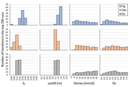
Figure 7.
Histograms of calibration parameter values (bi, usoilD, Dsmax, Ds) for the top 100 iterations of each discharge timeseries (Qg, Qgs, Qs).
Since every parameter iteration gives three KGE values, one for each timeseries compared to a modeled timeseries result, we compute the percent difference between KGE values per iteration (Figure 8). We aim to determine the effects that SWOT temporal sampling, SWOT uncertainty, and both SWOT temporal and uncertainty combined have on KGE values for all 10,000 modeled iterations. Do only the top iterations have comparable KGE values? How do all iterations compare to one another? Figure 8 is a density curve for all three percent difference comparisons, and thus the area under each curve is equal to 1. Taking the area under the curve between ± 30% difference indicates that 96% of iterations have less than 30% absolute difference when only temporal sampling differences (Qg vs. Qgs) are considered. Meanwhile, 62% of iterations have less than 30% absolute difference when just uncertainty is considered (Qgs vs. Qs), and 70% of iterations have less than 30% absolute difference when both sampling and uncertainty are considered (Qg vs. Qs). Subtracting KGE values from each other per iteration and taking the average of these values gives –0.01, 0.1, and 0.09 for Qg – Qgs, Qgs – Qs, and Qg – Qs, respectively. The comparisons involving uncertainty both have density curves that are skewed to the right with most percent differences greater than zero, indicating that comparing Qm with Qg or Qgs almost always gives a higher median KGE than comparing Qm with Qs, as expected. Moreover, 68% of iterations lie to the left of zero comparing Qg vs. Qgs KGE values, indicating that often, Qgs gives a higher KGE value than Qg. Since adding temporal variation (Qg vs. Qgs) tends to lead to negative percent differences and adding uncertainty (Qgs vs. Qs) tends to lead to larger positive percent differences, logically, adding the two together (Qg vs. Qs) would lead to positive percent differences as well, but not as large in magnitude as uncertainty by itself; therefore, more iterations have a larger percent difference for Qgs vs. Qs than Qg vs. Qs.
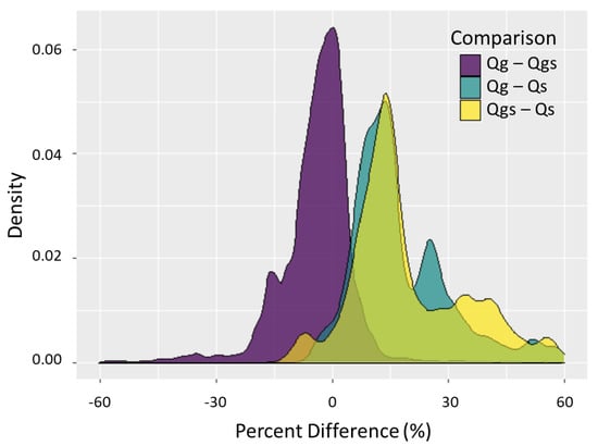
Figure 8.
Density curve of percent difference among the different timeseries median KGE values (Qg vs. Qgs, Qg vs. Qs, Qgs vs. Qs) for 10,000 iterations. The area under each curve is equal to 1.0, representing the density of iterations within certain percent errors, although outliers are not shown.
These results lead to the question: What are the implications of these differing KGE results for calibrated models in a practical sense? For the optimal parameter sets determined by KGE for models A, B, and C, the KGE values for each model timeseries compared to Qg, Qgs, or Qs are within ±0.03 of each other (Table S2). How do the models compare for metrics such as annual maximum and mean annual flows? We compare each modeled annual hydrograph for all 39 gauges with the truth timeseries, Qg, and compute the percent difference among them for all 9 years, giving 351 data points per statistic/model comparison shown in histograms (Figure 9). When the percent difference between Qg and model A is calculated, 68% of mean annual flow statistics lie within ±30% difference of the truth. Comparing with models B and C give similar results, with 69% and 71% of values within a ±30% difference, respectively. For mean annual flow, no obvious skew toward under or over estimation of the model discharge compared to Qg discharge exists. Annual maximum values give percent errors that are skewed to the right; model discharges tend to underestimate peak flows, regardless of the parameter sets selected. Seventy-five percent, 68%, and 76% of annual maximums for models A, B, and C, respectively, give positive percent errors. It is interesting to note that since models A and C have the same optimal values for controlling parameters, bi and usoilD, their values are more similar, as evident in the shape of their histograms. When median values of the annual statistics for the 39 gauges are analyzed, on average, models A and C only differ by about 1% for each statistic (Table S2). Model B gives a slightly higher mean annual flow value averaged over the 9-year period than models A and C (1% and 2% difference respectively) while having an approximately 10% difference from the two models regarding annual peak flow. In general, model B indicates that calibrating a model based on SWOT temporal sampling alone (Qgs) could produce hydrograph values with a more accurate representation of peak flows.
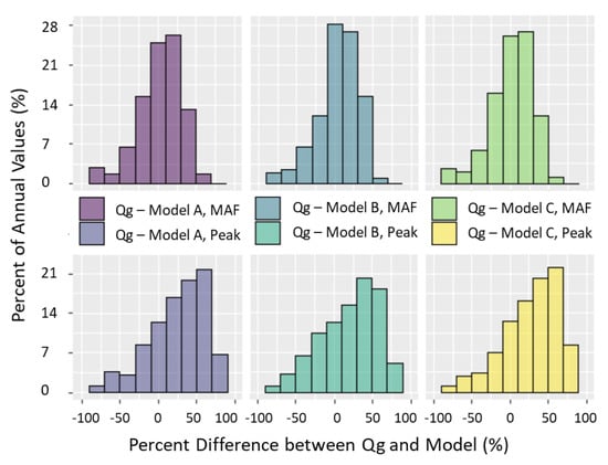
Figure 9.
Histograms of percent differences between annual Qg hydrograph statistics and annual modeled hydrograph (A, B, C) statistics, mean annual flow (MAF), and annual peak flow for the years 2010–2018. Each histogram has 351 comparisons, and the y-axis gives the percent of these values in each bin.
Except for bi, calibrated parameters are spatially the same throughout the entire basin; thus, we also investigated KGE as a function of drainage area to determine if each model varied in performance for upstream vs. downstream locations (Figure S1). Although no significant trendline was discernable for any of the models, upstream locations with smaller drainage areas have a wider spread of KGE values; however, high drainage area gauges are not as represented among the selected gauges. The plot does solidify the trends observed for the top three models: A, B, and C. Model C often gives the worst KGE value of the three. Model B tends to have the best KGE value for each location, although model A often has comparative values to model B as well.
3.3. Sensitivity and Validation Analysis
Since currently, the SWOT mission is expected to last at least 3 years, we scale down the amount of measurements for our calibration experiment from 9 years to 3 years to see if/how results change. We test 3 periods of 3 years (2010–2012, 2013–2015, 2016–2018) and find that the median and maximum KGE values do not change drastically for the selected best iterations (Table S3). The most influential parameter on model results, usoilD, continues to exhibit the same pattern for best iterations among timeseries with a slightly larger range, obtaining values between 1.0 and 1.4 m, depending on the timeseries used, as opposed to between 1.2 and 1.4 m as in the 9-year experiment. bi’s range increased as well, ranging from 0.04 to 0.32 as the best selected iteration; 0.32 is selected once for the Qs comparison for test years 2013–2015, giving the lowest KGE value out of all the optimal sets. Dsmax has the same range as the best iterations previously (12–40 mm/d), while Ds expands its range to span all tested values (0.1–1.0). If the average median KGE value is taken over for the top 100 iterations for each ranking order (Qg, Qgs, Qs), median KGE values stay between 0.39 and 0.50 regardless of the time period tested (Table S4). Using 3 years instead of 9 years does decrease median KGE values slightly, but only on average by 0.04 points. Changing the time period tested for calibration does not change the model results significantly.
For validation purposes, we compare median and maximum KGE values for the 9-year study period using top iteration parameters gleaned from each calibration time period per timeseries (Table S5). Although we acknowledge that the tested 3-year calibration periods are within the 9-year period, two-thirds of the 9 years are unused in calibration. Therefore, for consistency’s sake in comparing KGE values, we use the 9-year window as the study period regardless of calibration length. On average, 9-year median and maximum KGE values decrease by 9% and 5%, respectively, when comparing results from the 9-year calibration top parameters with those from any given iteration or timeseries from the 3-year calibration top parameters. For the study period, 9-year median KGE values are within 0.36–0.50 and 9-year maximum KGE values are within 0.62–0.79 when optimizing the model from a 3-year calibration period. The model performance decreases slightly when only 3 years are used for calibration compared to when all 9 years are calibrated.
4. Discussion
Since the best parameter iterations are selected based on the highest median KGE values, and it appears Qgs can often outperform Qg when compared to Qm to calculate KGE, a closer inspection on the nuances of each timeseries is necessary. How could a KGE value for Qgs vs. Qm be greater than for Qg vs. Qm? KGE values are calculated by comparing pairs of discharge values. Thus, Qm would be paired with Qg discharge daily. The Qgs timeseries has the same discharge values as Qg, which is only sampled on days that SWOT will observe each gauge location. To calculate KGE with this irregular timeseries, Qm values are also sampled on days that SWOT would observe them and KGE is calculated based on those pairs. The same is so for Qs. In [19], it was found that only 8% of monthly maximum discharges would be directly captured by SWOT overpasses, indicating that Qgs and Qs would not capture most peak flow events. Since modeled values more closely match USGS discharge values during low-flow and non-peak periods (Figure 5), it is conceivable that Qgs would provide a better KGE value than directly comparing the entire Qg timeseries with the entire Qm timeseries. A better KGE value from Qgs does not necessarily indicate better model performance overall; as discussed before in Figure 6, calibrating according to Qg does produce more robust model parameters. Qgs tends to give not only better KGE values, but also more accurate annual maximum flow values, although less discharge pairs are used to determine the KGE value that selects the iteration for optimal parameters. Since Qs values have an added layer of uncertainty with a Gaussian error added indicating a negative bias and larger spread, Qs discharge is not as analogous to Qm, and the KGE values are generally lower.
The Ohio River network is influenced by many man-made river structures, including reservoirs, dams, and river locks. These structures have been found to have an influence on hydrologic model calibration [43]. Specifically, they calibrate the VIC model with and without accounting for man-made structures and find that the calibration process compensates for the absence of reservoirs by selecting parameter values that imitate the alterations caused by reservoirs. Reservoirs increase evaporation and delay peak flows; thereby, parameter values are selected that increase infiltration, baseflow, and soil water storage capacity. In this study, selected values of bi, usoilD, Dsmax, and Ds may be influenced by the lack of accounting for reservoirs and other man-made structures in the HRR-VIC model.
We recognize that other hydrologic models may give different discharge estimations and KGE values higher than those reported in this study. Ref. [25] reports that the main sources of global hydrologic model discharge errors are precipitation and water budget parameters uncertainty in their experiment. It is likely that climatic forcings such as these, in addition to the calibrated parameters, also impact KGE values here. While we provide error metrics for the gauge calibration results, we do not explore the influence of model structure or model forcings on overall uncertainty. Here, we focus on model parameter uncertainty with SWOT-derived discharges. The focus of this experiment is not primarily on how well the hydrologic model performed but rather how the calibration results from different timeseries (Qg, Qgs, Qs) compare to one another.
5. Conclusions
Calibrating a model using discharge timeseries derived from the SWOT satellite’s irregular sampling frequency results in equivalent and sometimes better median KGE values throughout the 39 gauge locations within the Ohio River Basin as compared to calibrating the model with daily USGS discharge timeseries. In fact, KGE values increase on average by 0.01 when the model is calibrated using USGS discharges sampled based on SWOT overpasses as compared to the full daily record of discharges. Analyzing 10,000 model iterations shows that 93% of parameter iterations have KGE values with absolute percent differences less than 20% considering only SWOT temporal sampling. Calibrating the model with a timeseries attuned to SWOT temporal sampling and projected uncertainty decreases the top 100 parameter iteration KGE values by an average of 0.03 points compared to KGE values resulting from using the full USGS daily discharge record, and it decreases an average of 0.04 points compared to using the SWOT sampled USGS daily discharge record. Annual mean and peak flow values at each gauge from each of the top parameter iterations selected per timeseries have an average percent difference of less than 10%. Overall, these differences are minor and suggest that calibrating a hydrologic model with SWOT-derived discharge series (i.e., timeseries that have SWOT temporal sampling and/or projected uncertainties) can result in model performance that is similar to a model calibrated using daily in situ measurements. In addition to similar model performance, calibrating with SWOT-derived discharges results in similar, controlling, parameter values for upper soil layer depth (usoilD) and the variable infiltration curve parameter (bi). Despite their irregular sampling frequency and likely uncertainties, SWOT-derived discharges have the potential to capture streamflow characteristics that are sufficient for applications requiring hydrologic model calibration. This study also investigated calibration sensitivity due to sampling period, specifically different 3-year periods within the 9-year study period, and found only minimal impacts on calibrated model performance or selected parameter values. In summary, coupling hydrologic models with SWOT satellite observations will pave the way toward unprecedented advances in understanding river discharge dynamics, water resources, and flood risk from regional to global scales.
Supplementary Materials
The following are available online at https://www.mdpi.com/2072-4292/12/19/3241/s1, Table S1: Detailed USGS Gauge Information, Table S2: KGE and Annual Statistics for Top Iterations, Table S3: Selected Parameters and KGE Sensitivity Analysis, Table S4: Top 100 Iteration Sensitivity Analysis, Figure S1: Kling-Gupta Efficiency (KGE) values vs drainage area for all three calibration methods.
Author Contributions
Individual contributions are as follows: Conceptualization, C.N. and E.B.; methodology, E.B., C.N. and D.F.; software, E.B., D.F. and C.N.; validation, C.N., E.B. and D.F.; formal analysis, C.N.; investigation, C.N.; resources, C.N., E.B. and D.F.; data curation, C.N.; writing—original draft preparation, C.N.; writing—review and editing, C.N., E.B. and D.F.; visualization, C.N.; supervision, E.B.; project administration, E.B. and C.N.; funding acquisition, C.N. and E.B. All authors have read and agreed to the published version of the manuscript.
Funding
This research was funded by the National Science Foundation Graduate Research Fellowship Program, Grant No. 1451070. Any opinions, findings, and conclusions or recommendations expressed in this material are those of the authors and do not necessarily reflect the views of the National Science Foundation. Support for this research was also provided by NASA’s SWOT Science Team and Applied Sciences Programs, Grant No. NNX16AQ39G.
Conflicts of Interest
The authors declare no conflict of interest. The funders had no role in the design of the study; in the collection, analyses, or interpretation of data; in the writing of the manuscript, or in the decision to publish the results.
References
- Feng, D.; Beighley, E. Identifying uncertainties in hydrologic fluxes and seasonality from hydrologic model components for climate change impact assessments. Hydrol. Earth Syst. Sci. 2020, 24, 2253–2267. [Google Scholar] [CrossRef]
- Andreadis, K.M.; Schumann, G.J.P. Estimating the impact of satellite observations on the predictability of large-scale hydraulic models. Adv. Water Resour. 2014, 73, 44–54. [Google Scholar] [CrossRef]
- Beighley, R.E.; Eggert, K.G.; Dunne, T.; He, Y.; Gummadi, V.; Verdin, K.L. Simulating hydrologic and hydraulic processes throughout the Amazon River Basin. Hydrol. Process. 2009, 23, 1221–1235. [Google Scholar] [CrossRef]
- Chawla, I.; Karthikeyan, L.; Mishra, A.K. A review of remote sensing applications for water security: Quantity, quality, and extremes. J. Hydrol. 2020, 585, 124826. [Google Scholar] [CrossRef]
- Brêda, J.P.L.F.; Paiva, R.C.D.; Bravo, J.M.; Passaia, O.A.; Moreira, D.M. Assimilation of Satellite Altimetry Data for Effective River Bathymetry. Water Resour. Res. 2019, 55, 7441–7463. [Google Scholar] [CrossRef]
- Domeneghetti, A.; Tarpanelli, A.; Grimaldi, L.; Brath, A.; Schumann, G. Flow Duration Curve from Satellite: Potential of a Lifetime SWOT Mission. Remote Sens. 2018, 10, 1107. [Google Scholar] [CrossRef]
- Gleason, C.J.; Wada, Y.; Wang, J. A Hybrid of Optical Remote Sensing and Hydrological Modeling Improves Water Balance Estimation. J. Adv. Modeling Earth Syst. 2018, 10, 2–17. [Google Scholar] [CrossRef]
- Liu, G.; Schwartz, F.W.; Tseng, K.-H.; Shum, C.K. Discharge and water-depth estimates for ungauged rivers: Combining hydrologic, hydraulic, and inverse modeling with stage and water-area measurements from satellites. Water Resour. Res. 2015, 51, 6017–6035. [Google Scholar] [CrossRef]
- Pedinotti, V.; Boone, A.; Ricci, S.; Biancamaria, S.; Mognard, N. Assimilation of satellite data to optimize large-scale hydrological model parameters: A case study for the SWOT mission. Hydrol. Earth Syst. Sci. 2014, 18, 4485–4507. [Google Scholar] [CrossRef]
- Demaria, E.M.; Nijssen, B.; Wagener, T. Monte Carlo sensitivity analysis of land surface parameters using the Variable Infiltration Capacity model. J. Geophys. Res. Atmos. 2007, 112, D11113. [Google Scholar] [CrossRef]
- Huang, M.; Liang, X. On the assessment of the impact of reducing parameters and identification of parameter uncertainties for a hydrologic model with applications to ungauged basins. J. Hydrol. 2006, 320, 37–61. [Google Scholar] [CrossRef]
- Oubeidillah, A.A.; Kao, S.C.; Ashfaq, M.; Naz, B.S.; Tootle, G. A large-scale, high-resolution hydrological model parameter data set for climate change impact assessment for the conterminous US. Hydrol. Earth Syst. Sci. 2014, 18, 67–84. [Google Scholar] [CrossRef]
- Troy, T.J.; Wood, E.F.; Sheffield, J. An efficient calibration method for continental-scale land surface modeling. Water Resour. Res. 2008, 44. [Google Scholar] [CrossRef]
- Yang, Y.; Pan, M.; Beck, H.E.; Fisher, C.K.; Beighley, R.E.; Kao, S.-C.; Hong, Y.; Wood, E.F. In Quest of Calibration Density and Consistency in Hydrologic Modeling: Distributed Parameter Calibration against Streamflow Characteristics. Water Resour. Res. 2019, 55, 7784–7803. [Google Scholar] [CrossRef]
- Biancamaria, S.; Lettenmaier, D.P.; Pavelsky, T.M. The SWOT Mission and Its Capabilities for Land Hydrology. Surv. Geophys. 2016, 37, 307–337. [Google Scholar] [CrossRef]
- Durand, M.; Gleason, C.J.; Garambois, P.A.; Bjerklie, D.; Smith, L.C.; Roux, H.; Rodriguez, E.; Bates, P.D.; Pavelsky, T.M.; Monnier, J.; et al. An intercomparison of remote sensing river discharge estimation algorithms from measurements of river height, width, and slope. Water Resour. Res. 2016, 52, 4527–4549. [Google Scholar] [CrossRef]
- Hagemann, M.W.; Gleason, C.J.; Durand, M.T. BAM: Bayesian AMHG-Manning Inference of Discharge Using Remotely Sensed Stream Width, Slope, and Height. Water Resour. Res. 2017, 53, 9692–9707. [Google Scholar] [CrossRef]
- Pavelsky, T.M.; Durand, M.T.; Andreadis, K.M.; Beighley, R.E.; Paiva, R.C.D.; Allen, G.H.; Miller, Z.F. Assessing the potential global extent of SWOT river discharge observations. J. Hydrol. 2014, 519, 1516–1525. [Google Scholar] [CrossRef]
- Nickles, C.; Beighley, E.; Zhao, Y.; Durand, M.; David, C.; Lee, H. How does the unique space-time sampling of the SWOT mission influence river discharge series characteristics? Geophys. Res. Lett. 2019, 46, 8154–8161. [Google Scholar] [CrossRef]
- Baratelli, F.; Flipo, N.; Rivière, A.; Biancamaria, S. Retrieving river baseflow from SWOT spaceborne mission. Remote Sens. Environ. 2018, 218, 44–54. [Google Scholar] [CrossRef]
- Solander, K.C.; Reager, J.T.; Famiglietti, J.S. How well will the Surface Water and Ocean Topography (SWOT) mission observe global reservoirs? Water Resour. Res. 2016, 52, 2123–2140. [Google Scholar] [CrossRef]
- Frasson, R.P.D.M.; Schumann, G.J.-P.; Kettner, A.J.; Brakenridge, G.R.; Krajewski, W.F. Will the Surface Water and Ocean Topography (SWOT) satellite mission observe floods? Geophys. Res. Lett. 2019, 46. [Google Scholar] [CrossRef]
- Getirana, A.C.V. Integrating spatial altimetry data into the automatic calibration of hydrological models. J. Hydrol. 2010, 387, 244–255. [Google Scholar] [CrossRef]
- Sun, W.; Fan, J.; Wang, G.; Ishidaira, H.; Bastola, S.; Yu, J.; Fu, Y.H.; Kiem, A.S.; Zuo, D.; Xu, Z. Calibrating a hydrological model in a regional river of the Qinghai–Tibet plateau using river water width determined from high spatial resolution satellite images. Remote Sens. Environ. 2018, 214, 100–114. [Google Scholar] [CrossRef]
- Wongchuig-Correa, S.; Cauduro Dias de Paiva, R.; Biancamaria, S.; Collischonn, W. Assimilation of future SWOT-based river elevations, surface extent observations and discharge estimations into uncertain global hydrological models. J. Hydrol. 2020, 590, 125473. [Google Scholar] [CrossRef]
- Huang, Q.; Long, D.; Du, M.; Han, Z.; Han, P. Daily Continuous River Discharge Estimation for Ungauged Basins Using a Hydrologic Model Calibrated by Satellite Altimetry: Implications for the SWOT Mission. Water Resour. Res. 2020, 56, e2020WR027309. [Google Scholar] [CrossRef]
- Liang, X.; Lettenmaier, D.P.; Wood, E.F.; Burges, S.J. A simple hydrologically based model of land surface water and energy fluxes for general circulation models. J. Geophys. Res. Atmos. 1994, 99, 14415–14428. [Google Scholar] [CrossRef]
- Allen, G.H.; Pavelsky, T.M. Global extent of rivers and streams. Science 2018, 361, 585–588. [Google Scholar] [CrossRef]
- Centre National d’Etudes Spatiales. SWOT Orbit: Ground Track and Swath Files. 2018. Available online: https://www.aviso.altimetry.fr/en/missions/future-missions/swot/orbit.html (accessed on 1 May 2018).
- Ray, R.L.; Beighley, R.E.; Yoon, Y. Integrating Runoff Generation and Flow Routing in Susquehanna River Basin to Characterize Key Hydrologic Processes Contributing to Maximum Annual Flood Events. J. Hydrol. Eng. 2016, 21, 04016026. [Google Scholar] [CrossRef]
- Shangguan, W.; Dai, Y.; Duan, Q.; Liu, B.; Yuan, H. A global soil data set for earth system modeling. J. Adv. Modeling Earth Syst. 2014, 6, 249–263. [Google Scholar] [CrossRef]
- Xia, Y. NCEP/EMC, NLDAS Primary Forcing Data L4 Hourly 0.125 × 0.125 degree V002, Edited by David Mocko, NASA/GSFC/HSL, Greenbelt, Maryland, USA, Goddard Earth Sciences Data and Information Services Center (GES DISC). 2009. Available online: https://disc.gsfc.nasa.gov/datasets/NLDAS_FORA0125_H_002/summary (accessed on 1 October 2019). [CrossRef]
- Xia, Y.; Mitchell, K.; Ek, M.; Sheffield, J.; Cosgrove, B.; Wood, E.; Luo, L.; Alonge, C.; Wei, H.; Meng, J.; et al. Continental-scale water and energy flux analysis and validation for the North American Land Data Assimilation System project phase 2 (NLDAS-2): 1. Intercomparison and application of model products. J. Geophys. Res. Atmos. 2012, 117, D03109. [Google Scholar] [CrossRef]
- Qin, Y.; Abatzoglou, J.T.; Siebert, S.; Huning, L.S.; AghaKouchak, A.; Mankin, J.S.; Hong, C.; Tong, D.; Davis, S.J.; Mueller, N.D. Agricultural risks from changing snowmelt. Nat. Clim. Chang. 2020, 10, 459–465. [Google Scholar] [CrossRef]
- US Department of Agriculture (USDA). National Engineering Handbook. Snowmelt. 2004. Available online: https://directives.sc.egov.usda.gov/OpenNonWebContent.aspx?content=17753.wba (accessed on 1 April 2020).
- Anderson, E. National Weather Service River Forecast System—Snow Accumulation and Ablation Model; NOAA Tech. Memo. NWS HYDRO-17; U.S. Dep. Commerce: Silver Springs, MD, USA, 1973; 217p.
- Barnhart, T.B.; Molotch, N.P.; Livneh, B.; Harpold, A.A.; Knowles, J.F.; Schneider, D. Snowmelt rate dictates streamflow. Geophys. Res. Lett. 2016, 43, 8006–8016. [Google Scholar] [CrossRef]
- Rango, A.; Martinec, J. Revisiting the degree-day method for snowmelt computations. J. Am. Water Resour. Assoc. 1995, 31, 657–669. [Google Scholar] [CrossRef]
- Nickles, C.; Beighley, E.; Feng, D. Hillslope River Routing Variable Infiltration Capacity Model (HRR-VIC) and Calibration Results. Available online: http://www.hydroshare.org/resource/172bf3533b1d46ea8d89feea51d44fb7 (accessed on 21 September 2020). [CrossRef]
- Clapp, R.B.; Hornberger, G.M. Empirical equations for some soil hydraulic properties. Water Resour. Res. 1978, 14, 601–604. [Google Scholar] [CrossRef]
- Gupta, H.V.; Kling, H.; Yilmaz, K.K.; Martinez, G.F. Decomposition of the mean squared error and NSE performance criteria: Implications for improving hydrological modelling. J. Hydrol. 2009, 377, 80–91. [Google Scholar] [CrossRef]
- Knoben, W.J.M.; Freer, J.E.; Woods, R.A. Technical note: Inherent benchmark or not? Comparing Nash–Sutcliffe and Kling–Gupta efficiency scores. Hydrol. Earth Syst. Sci. 2019, 23, 4323–4331. [Google Scholar] [CrossRef]
- Dang, T.D.; Kamal Chowdhury, A.F.M.; Galelli, S. On the representation of water reservoir storage and operations in large-scale hydrological models: Implications on model parameterization and climate change impact assessments. Hydrol. Earth Syst. Sci. 2020, 24, 397–426. [Google Scholar] [CrossRef]
© 2020 by the authors. Licensee MDPI, Basel, Switzerland. This article is an open access article distributed under the terms and conditions of the Creative Commons Attribution (CC BY) license (http://creativecommons.org/licenses/by/4.0/).