Evaluation of Assimilating FY-3C MWHS-2 Radiances Using the GSI Global Analysis System

Abstract

The MicroWave Humidity Sounder 2 (MWHS-2) onboard the FY-3C satellite provides an extra important data source for atmospheric water vapor monitoring besides the Microwave Humidity Sounder (MHS) and the Advanced Technology Microwave Sounder (ATMS). This paper introduces MWHS-2 radiance data into the community Gridpoint Statistical Interpolation (GSI) global analysis system. More than one-year cycling assimilation experiments with and without MWHS-2 data are performed. Results show that MWHS-2 has similar data quality to MHS and ATMS. The biases of MWHS-2 are stable except some sudden jumps that can be removed nicely by the variational bias correction scheme within GSI. Assimilating MWHS-2 makes the 6-h forecasts fit more closely to radiosonde observations, with a reduction of 0.55–1% for the observation-minus-simulation standard deviation of specific humidity. The 500 hPa geopotential height anomaly correlation scores are increased by around 0.006 for the 144-h forecast, indicating that assimilating MWHS-2 may also help to improve 3–8-day forecasts.

1. Introduction

Millions of satellite observations are assimilated operationally in numerical weather prediction (NWP) centers. Among these observations, microwave sounding measurements, including the Advanced Microwave Sounding Unit A (AMSU-A), the Microwave Humidity Sounder (MHS) and the Advanced Technology Microwave Sounder (ATMS), play an important role in the forecast performance [1].

The Microwave Humidity Sounder-2 (MWHS-2), onboard the Feng-Yun-3C (FY-3C) polar orbiting satellite launched by the China Meteorological Administration (CMA) in September 2013, provides not only humidity channels centered at 183 GHz, the same as MHS, but also temperature channels (also sensitive to low-level humidity) centered on a single oxygen line at 118 GHz. MWHS-2 is the second generation of Chinese microwave sounding instruments [2]. The data quality of the first-generation instrument, the MicroWave Humidity Sounder (MWHS) onboard the FY-3A satellite, was evaluated based on first-guess departures (observed radiance minus the simulated equivalents from short-range forecasts, O−B) calculated from the European Centre for Medium-range Weather Forecasts (ECMWF) Integrated Forecasting System (IFS) [3]. Neutral to slightly positive impact on humidity and wind forecasts was shown by assimilating MWHS observations from FY-3A and FY-3B using ECMWF IFS in [4]. MWHS-2 has similar abilities to ATMS onboard the Suomi National Polar-orbiting Partnership (SNPP) [2]. The long-term performance of MWHS-2 instruments was evaluated using statistics of observation departures from the ECMWF and Met Office global systems, and it was found that MWHS-2 had good quality for most channels except some jumps during 2016 caused by the change of instrument environment temperature [5]. The assessment of data quality and all-sky assimilation trials using ECMWF IFS revealed the benefits of MWHS-2 data assimilation (DA) to forecast accuracy [6]. The UK Met Office started the operational assimilation of MWHS-2 observations in its global system in March 2016 and found that MWHS-2 contributed to the 24-h forecast error reduction by 0.6% [7]. It is also found that the assimilation of MWHS improved the typhoon tracks, intensities, and precipitation forecasts in its regional assimilation and forecasting system [8]. Besides the use in weather forecasting fields, the MWHS and MWHS-2 instruments onboard FY-3B and FY-3C, respectively, have also been assimilated in the fifth-generation of ECMWF atmospheric reanalyses (ERA5) [9].

The CMA started to produce China’s first generation of a 40-year global atmospheric reanalysis (CRA-40) in 2014 [10]. MWHS-2 is an important potential data source for CRA-40. The main purpose of this paper is to introduce MWHS-2 data into the Gridpoint Statistical Interpolation (GSI) system, which was proposed to be used for CRA-40 production, and to evaluate the performance of MWHS-2 radiance DA.

The remainder of this paper is organized as follows: Section 2 describes the FY-3C MWHS-2 data, as well as other conventional and satellite observations, used in the experiments. Section 3 introduces MWHS-2 into the GSI global analysis system and describes the experimental design. Results are presented in Section 4, with discussion and conclusions given in Section 5 and Section 6.

2. Data

2.1. FY-3C MWHS-2

The MWHS-2 instrument onboard FY-3C, launched in September 2013, is a cross-track scanning radiometer on a morning orbit with an equator crossing time at approximately 10:15 AM (descending). It has 15 channels in total, including 5 channels in the 183 GHz water vapor band, 2 window channels centered at 89 GHz and 150 GHz, and 8 channels in the 118 GHz oxygen band [2]. MWHS-2 has 98 field of views (FOVs) in each scan line, with nadir spatial resolutions of 16 km at 150 and 183 GHz and 32 km at 89 and 118 GHz [6]. It is worth noting that it is the first time that the 118 GHz channels are available from a spacecraft, while the 183 GHz, 150 GHz and 89 GHz channels are similar to those of ATMS (see

Table 1. Microwave Humidity Sounder-2 (MWHS-2), Advanced Technology Microwave Sounder (ATMS), and Microwave Humidity Sounder (MHS) channel numbers, central frequencies, polarizations, and weighting function peak heights.

Channel Number			Central Frequency (GHz) and Polarization			Weight Function Peak Height (hPa)
MWHS-2	ATMS	MHS	MWHS-2	ATMS	MHS	MWHS-2	ATMS	MHS
1	16	1	89 (H)	88.2 (V)	89 (V)	-	-	-
2	-	-	118.75 ± 0.08 (V)	-	-	29.72	-	-
3	-	-	118.75 ± 0.2 (V)	-	-	75.65	-	-
4	-	-	118.75 ± 0.3 (V)	-	-	103.5	-	-
5	-	-	118.75 ± 0.8 (V)	-	-	265.0	-	-
6	-	-	118.75 ± 1.1 (V)	-	-	356.5	-	-
7	-	-	118.75 ± 2.5 (V)	-	-	Surface	-	-
8	-	-	118.75 ± 3.0 (V)	-	-	Surface	-	-
9	-	-	118.75 ± 5.0 (V)	-	-	Surface	-	-
10	17	2	150 (H)	165.5 (H)	157 (V)	Surface	Surface	Surface
11	22	3	183 ± 1.0 (V)	183 ± 1.0 (H)	183 ± 1.0 (H)	411.1	450.738	400
12	21	-	183 ± 1.8 (V)	183 ± 1.8 (H)		472.2	506.115	-
13	20	4	183 ± 3.0 (V)	183 ± 3.0 (H)	183 ± 3.0 (H)	616.6	606.847	600
14	19	-	183 ± 4.5 (V)	183 ± 4.5 (H)		701.2	695.847	-
15	18	5	183 ± 7.0 (V)	183 ± 7.0 (H)	190.31 (V)	795.0	790.017	800

). A full list of channel frequencies and the corresponding peaks of weight functions (WFs) are listed in Table 1. The WFs of MWHS-2 were calculated in [2] using the standard U.S. atmospheric profile, while those of ATMS are from [11]. More detailed instrument specification of MWHS-2 can be found in [12].

2.2. MHS

Observations from MHS instruments onboard the National Oceanic and Atmospheric Administration (NOAA)-19 satellite, and the meteorological operational satellite (MetOP)-A and MetOP-B are used for the comparison of assimilation impacts. As shown in Table 1, MHS has 2 window channels at 89 GHz and 157 GHz, and 3 water vapor channels at 183 ± 1.0, 183 ± 3.0 and 190.31 GHz with peaks of WFs at 400, 600, and 800 hPa, respectively. MHS is also a cross-track microwave radiometer with the same nadir spatial resolution as MWHS-2, but fewer FOVs (90), and thus smaller swath width (2250 km) than MWHS-2 (2700 km) [4]. The MHS observations used in this study have been downloaded from the NOAA Operational Model Archive and Distribution System (NOMDAS, https://nomads.ncep.noaa.gov).

2.3. ATMS

The ATMS instrument onboard the SNPP satellite is also used in this study for comparison with MWHS-2. ATMS has 22 channels, including 5 water vapor channels (18–22) the same as MWHS-2 (channels 11–15), 2 window channels at 88.2 GHz (channel 16) and 165.5 GHz (channel 17) similar to MWHS-2 channels 1 and 10, 10 temperature sounding channels (6–15) similar to AMSU-A (channels 5–14) [13]. It has 96 FOVs in each cross-track scan line, and the swath width is about 2500 km. The ATMS data have also been downloaded from NOAA NOMDAS.

2.4. Conventional and other Satellite Observations

Conventional observations (radiosonde, aircraft, surface synoptic observation, aviation routine weather report, ship, buoy etc.) and other satellite observations, including the Infrared Atmospheric Sounding Interferometer (IASI), the Atmospheric Infrared Sounder (AIRS) and atmospheric motion vectors (AMVs) used in this study have also been downloaded from NOMDAS.

2.5. ERA5 Reanalysis

The 6-hourly products of ERA5 [9] are used to compare with the results produced by the two experiments described in Section 3.3. The dataset was downloaded from the Copernicus Climate Data Store (CDS, https://cds.climate.copernicus.eu).

3. Data Assimilation System and Experimental Design

3.1. Data Assimilation and Forecasting System

The Community Gridpoint Statistical Interpolation system, version 3.6 (GSI-v3.6), is used to perform the DA experiments reported in Section 3.3. GSI-v3.6 supports three-dimensional variational (3DVar), 3D ensemble-variational, and 4D ensemble-variational techniques. 3DVar DA with observation departures calculated against the first guess at appropriate time (FGAT) technique [14,15] is used in the 6-hourly cycling system in this study. The analysis is performed four times per day (0000 UTC, 0600 UTC, 1200 UTC and 1800 UTC) with a time window of 6 h. Hourly forecasts from 1 to 9 h are used to calculate observation departures using the FGAT technique. GSI-3DVar [16] finds the statistically optimal solution (namely, the analysis) by minimizing an incremental cost function defined as:

$$J\left(x\right)=\frac{1}{2}{x}^{\mathrm{T}}{\mathrm{B}}^{-1}x+\frac{1}{2}{\left(\mathrm{H}x-y\right)}^{\mathrm{T}}{\mathrm{R}}^{-1}\left(\mathrm{H}x-y\right)+J_c$$

(1)

where x is the analysis increment, B is the background error covariance, H is the linearized observation operator, y is the observation departure (observation minus the equivalent value computed from the background), R is the observation error covariance, and J_c is a tangent-linear normal-mode constraint designed for incremental noise reduction and balance improvement (see details in [17]). The Community Radiative Transfer Model [18,19] is used as the observation operator for satellite radiance assimilation.

The forecast model used in this paper is the NOAA Environmental Modeling System framework-based Global Spectral Model (GSM), version 14.0.0, which was put into operation at the NCEP in June 2017. The model is configured following the NCEP Global Data Assimilation System (v14.0.0) settings, except that the spectral resolution is reduced to 574 truncations (T574, approximately 34 km grid spacing) and the near-surface sea temperature scheme is turned off. The model runs with two time-level semi-implicit semi-Lagrangian dynamics [20] with a time step of 900 s. It has 64 vertical levels, with the model top at 0.27 hPa. More details about GSM can be found at https://www.emc.ncep.noaa.gov/emc/pages/numerical_forecast_systems/gfs.php.

3.2. Introduction of MWHS-2 into GSI

GSI has the ability to assimilate various satellite observations, including those from AMSU-A, MHS, ATMS, IASI, AIRS, and so on. These observations are all read into GSI in the Binary Universal Form for the Representation of meteorological data (BUFR) file format. To assimilate MWHS-2 observations in GSI, the Hierarchical Data Format MWHS-2 data are firstly converted into BUFR format, and then an MWHS-2 assimilation interface along with quality control (QC) procedures is introduced into GSI following the assimilation scheme of MHS and AMSU-A.

We only use clear-sky MWHS-2 observations in this study. Channels 1 (89 GHz) and 10 (150 GHz) are used to calculate the total column precipitable water (TPW) index following the MHS scheme described in [21]. If the TPW index > 1, MWHS-2 observations from all channels except channels 3–6 for the same FOV are rejected. Then, the O−B check is performed to remove the outliers with limitations of 1 K, 3 K and 5 K for the temperature sounding channels (3–6), humidity sounding channels (11–15) and window channels (1–2 and 7–10), respectively.

The enhanced radiance variational bias correction (VarBC) scheme [22] with predictors of global offset, zenith angle, cloud liquid water, temperature lapse rate, square of the temperature lapse rate and scan-angle bias, is also performed for MWHS-2 assimilation in this study. For each channel, the bias model is described as a linear function of these predictors with coefficients optimally estimated in the variational analysis scheme as additional control variables.

3.3. Experimental Design

To evaluate the newly developed MWHS-2 assimilation interface and the performance of MWHS-2 assimilation, two long-term experiments are conducted covering July 1, 2016 to August 31, 2017. The first experiment, denoted as “CTRL”, assimilates all available global observations except MWHS-2, including conventional observations (radiosondes, aircraft, synoptic observations, ship, buoy etc.), microwave observations (AMSU-A, MHS and ATMS), infrared radiances (HIRS, IASI and AIRS), GPS Radio Occultation bending angle observations, AMVs, and ocean surface wind. Another experiment, denoted as “MWHS-2”, assimilates all observations in the “CTRL”, plus the FY-3C MWHS-2 radiances from 183 GHz channels (11–15) and 118 GHz channels (3–6). Both experiments are initialized by the CRA-40 model level product valid at 00Z on July 1, 2016. The first month is treated as a “spin-up” period, and thus not included in the following analysis of results.

4. Results

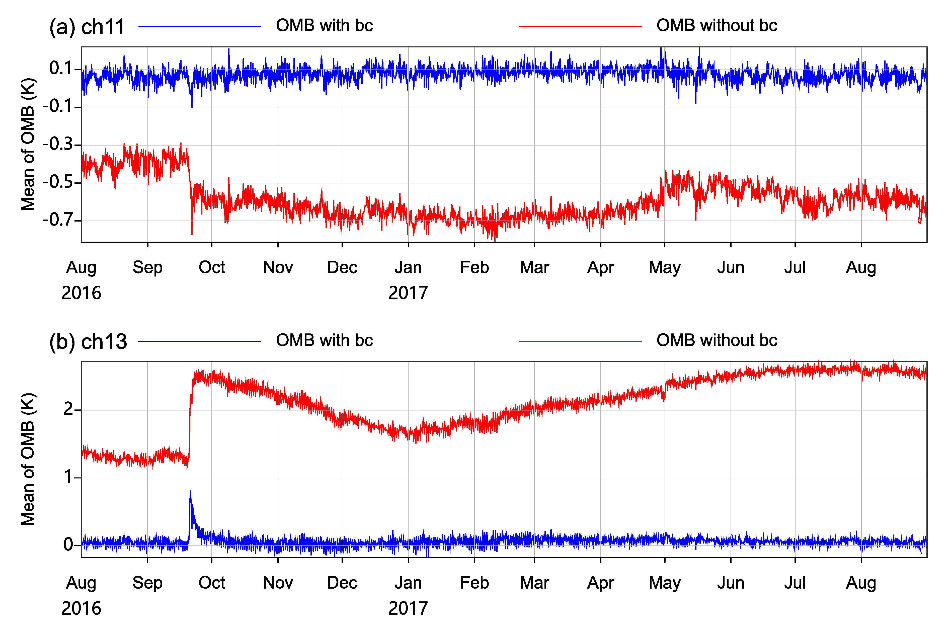
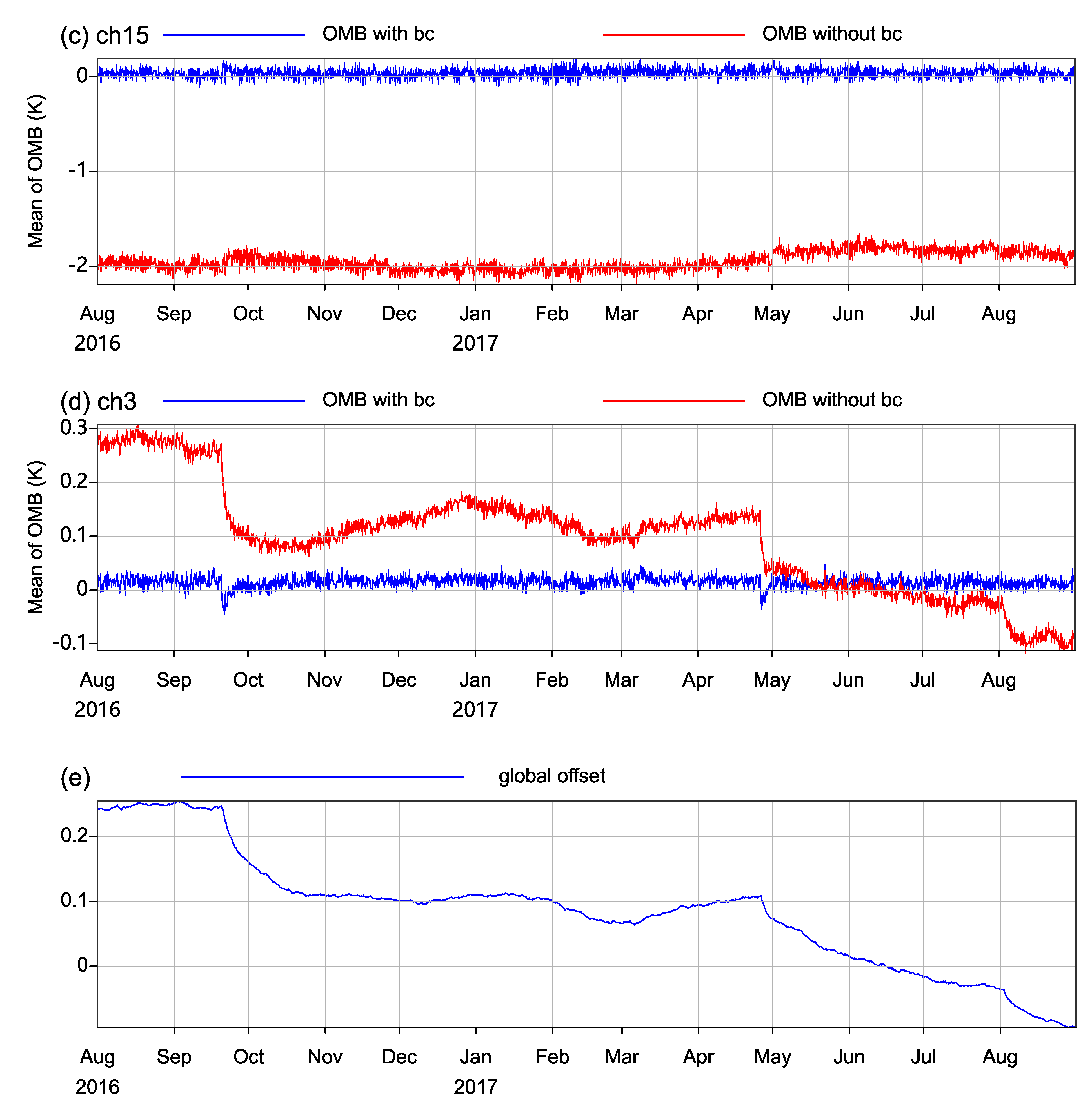
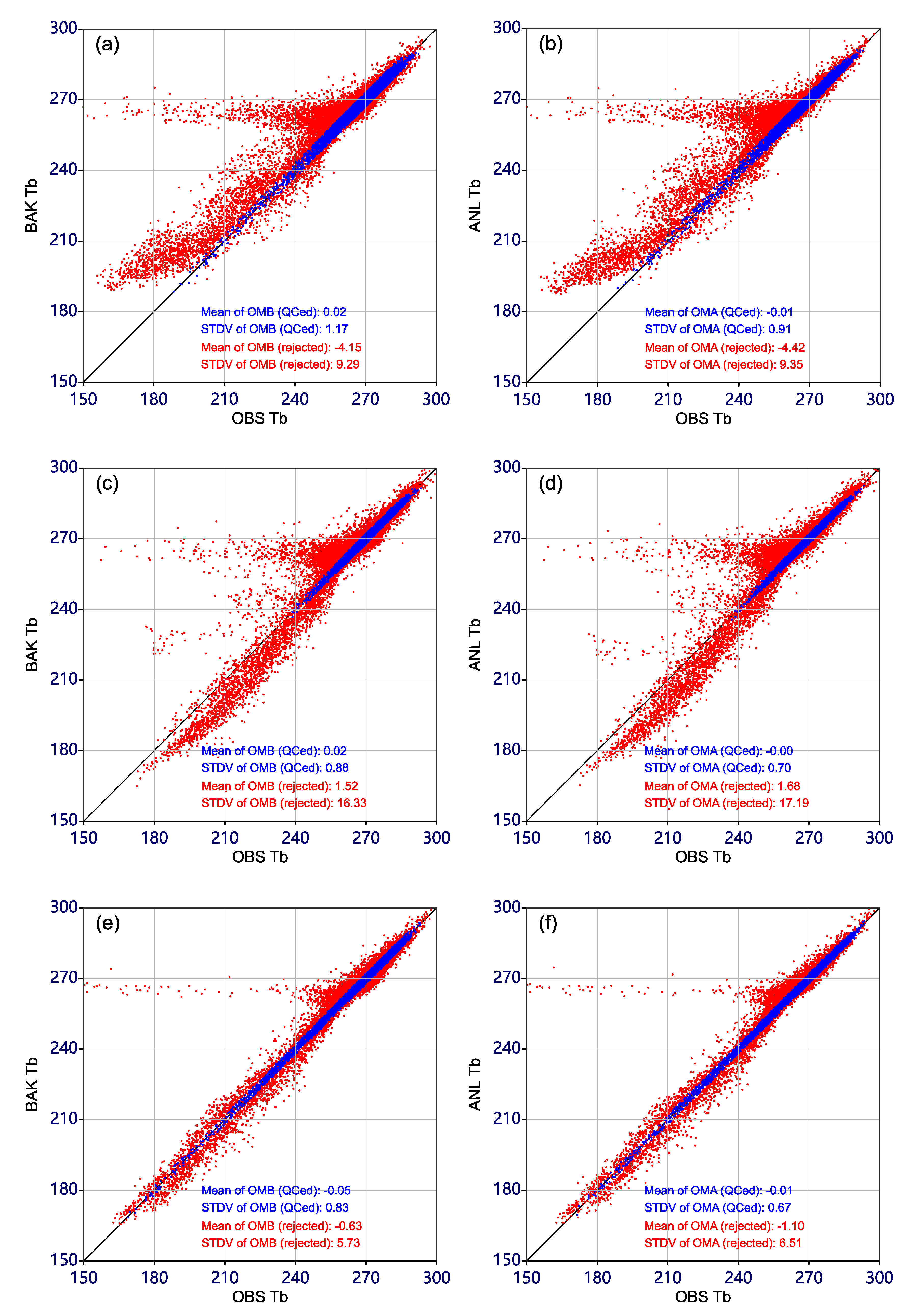
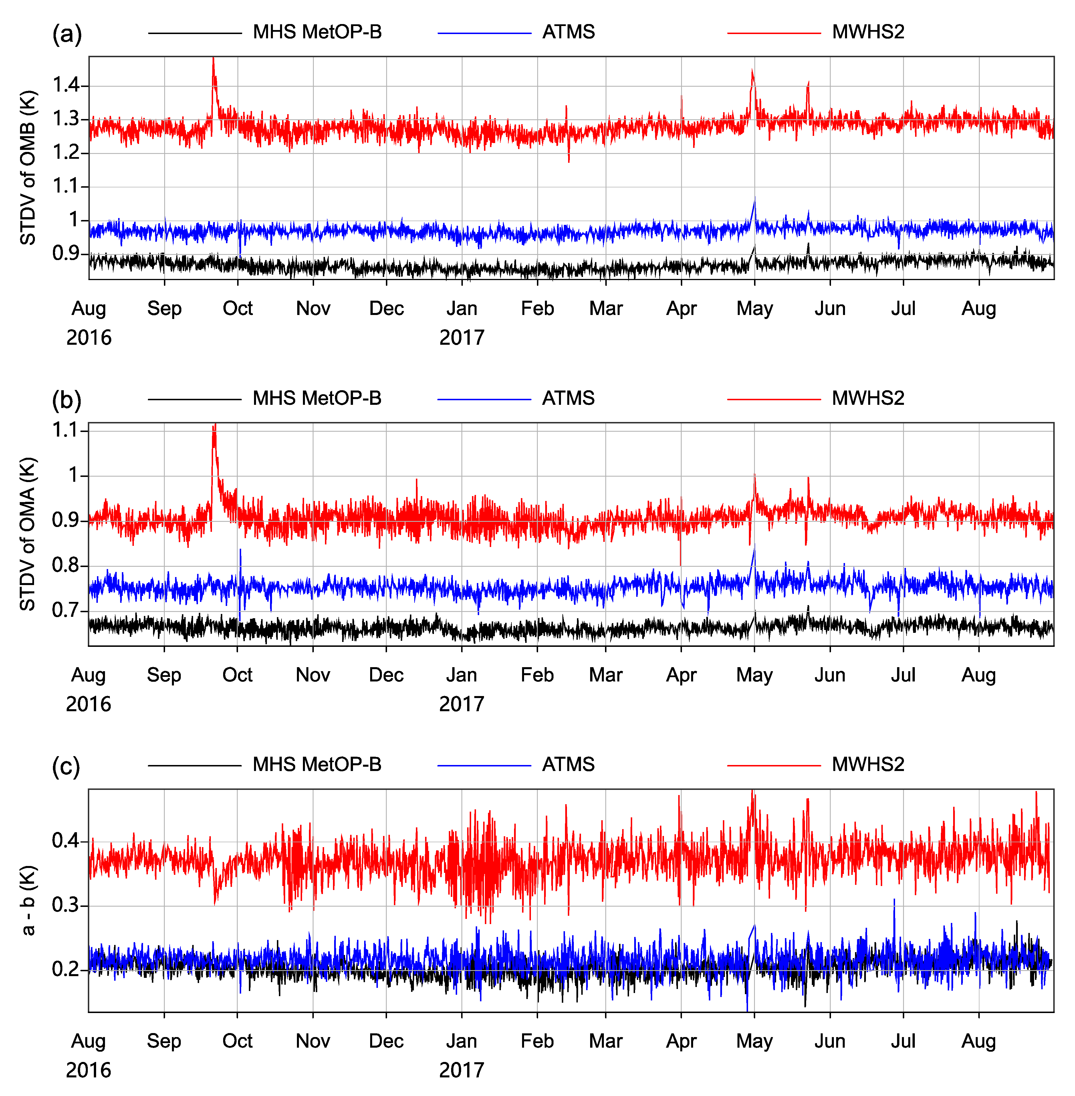
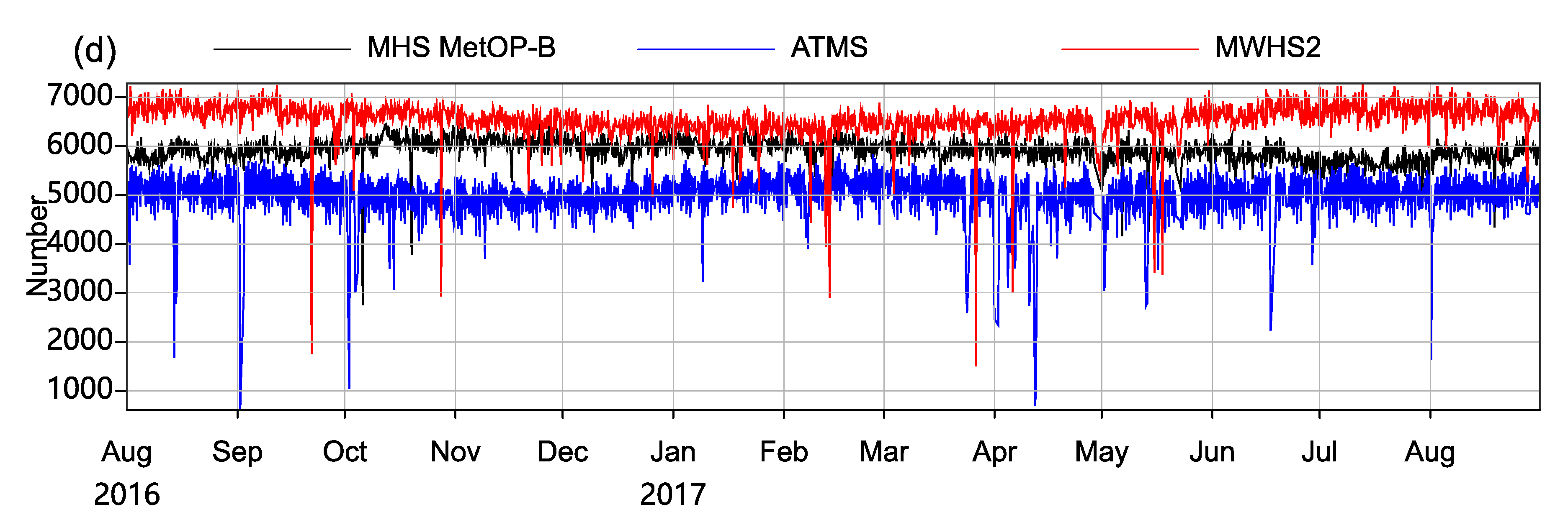
4.1. Performance of MWHS-2 VarBC and QC

Bias correction is an important procedure for satellite radiance assimilation. To check and evaluate the performance of VarBC for MWHS-2 observations, the time series of the global mean of O−B before and after VarBC are shown in Figure 1. A sudden bias jump for channels 11 and 13 at 183 GHz and channel 3 at 118 GHz can clearly be seen on 20 September 2016, which was also reported in [5,7]. This issue was found to be correlated with changes in the environment temperature of the instrument [5]. Two other bias jumps for channel 3 on 26 April 2017 and 3 August 2017 are also apparent in Figure 1d. The reason for these two bias jumps is still under investigation. They are, however, nicely removed with VarBC, as shown in Figure 1 (blue line). As described in Section 3.2, the bias is modeled as a linear function of predictors along with corresponding coefficients calculated during the analysis. Figure 1e shows the global offset coefficient for channel 3 used in VarBC scheme. It can be seen that the global offsets coefficients vary coincidently with changes of channel 3 observation minus background, indicating that the bias is well modeled and thus effectively removed. The one-year (1 August 2016 to 31 August 2017) average biases for channels 11, 13, 15 and 3 with VarBC are 0.07, 0.06, 0.04 and 0.01 K, respectively.

QC is another important procedure for MWHS-2 assimilation. Therefore, we compare the QC performance for MWHS-2 channel 15 observations from 21Z 31 July 2016 to 03Z 2 August 2016 (Figure 2a,b) with the equivalent channel 18 of SNPP ATMS (Figure 2c,d) and channel 5 of MetOP-B MHS (Figure 2e,f). It can be clearly seen that observations passing QC (blue points) fall on a diagonal line for MWHS-2, ATMS and MHS, while those rejected by QC (red points) are far away from the diagonal line. The mean and standard deviation (Stdv) of O−B for rejected and QCed observations are also given in Figure 2. The Stdv of O−B (QCed) for MWHS-2, ATMS and MHS is 1.17 K, 0.88 K and 0.83 K, respectively, while that of observation minus analysis (O−A) drops to 0.91 K, 0.70 K and 0.67 K, respectively.

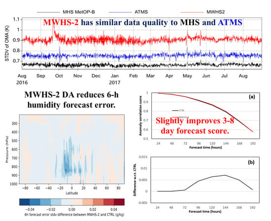
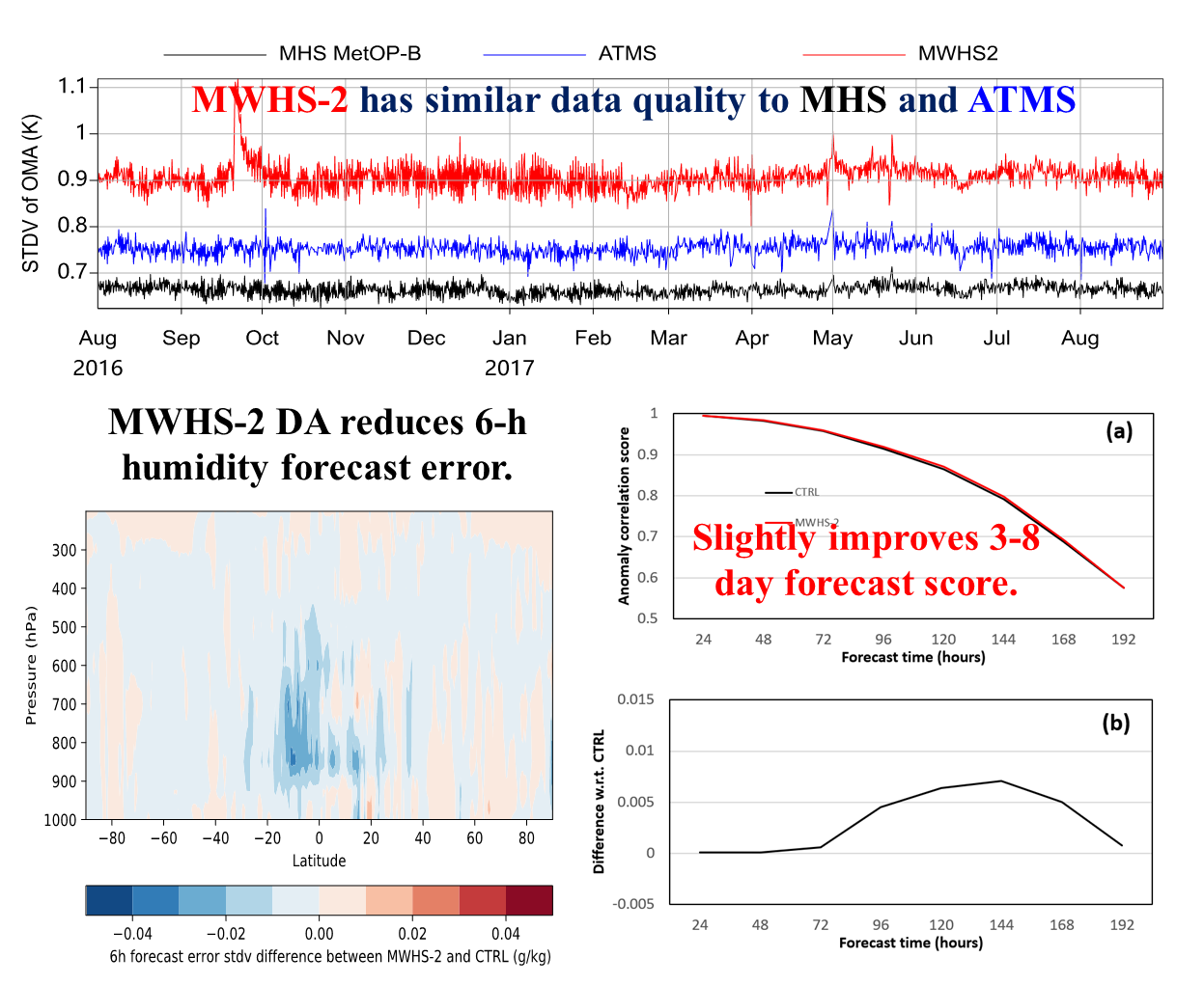
4.2. Analyses Statistics

The effect of MWHS-2 observation assimilation on analysis statistics is checked by comparison with the equivalent MetOP-B MHS and SNPP ATMS observations. As shown in Figure 3a, the time series of the Stdv of O−B with VarBC for MWHS-2 channel 13 (red line), along with the equivalent channel 20 of ATMS (blue line) and channel 4 of MHS (black line) are very stable over the period of the long-term experiment (August 2016 to August 2017), except for MWHS-2 on 20 September 2016 and 26 April 2017 when the bias jumps suddenly, as discussed in Section 4.1. A similar phenomenon can also be seen in Figure 3b for O−A. It is further apparent that the Stdv values of O−A for MWHS-2 (around 0.9 K), ATMS (around 0.75 K) and MHS (around 0.66 K) are smaller than those of O−B (around 1.3 K, 0.99 K and 0.89 K for MWHS-2, ATMS and MHS, respectively), which is expected. The Stdv reductions (differences between O−B and O−A) are also calculated (as shown in Figure 3c). The reductions for ATMS and MHS are both around 0.2 K, and smaller than that of MWHS-2 (around 0.38 K). These results are consistent with those of FY-3C MWHS-2 assimilation in the UM Met Office global model described in [7]. The number of observations used for the three instruments are shown in Figure 3d.

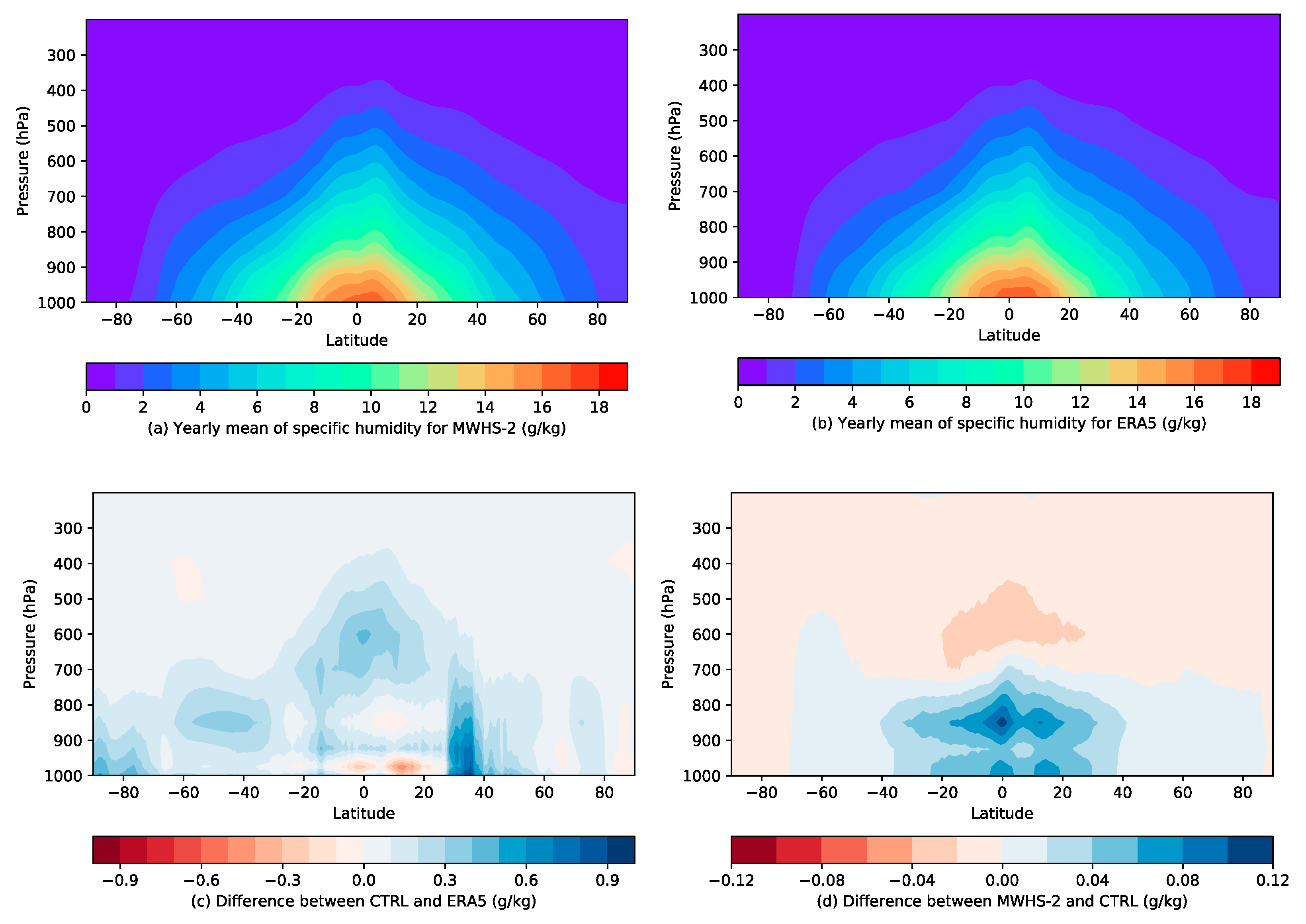
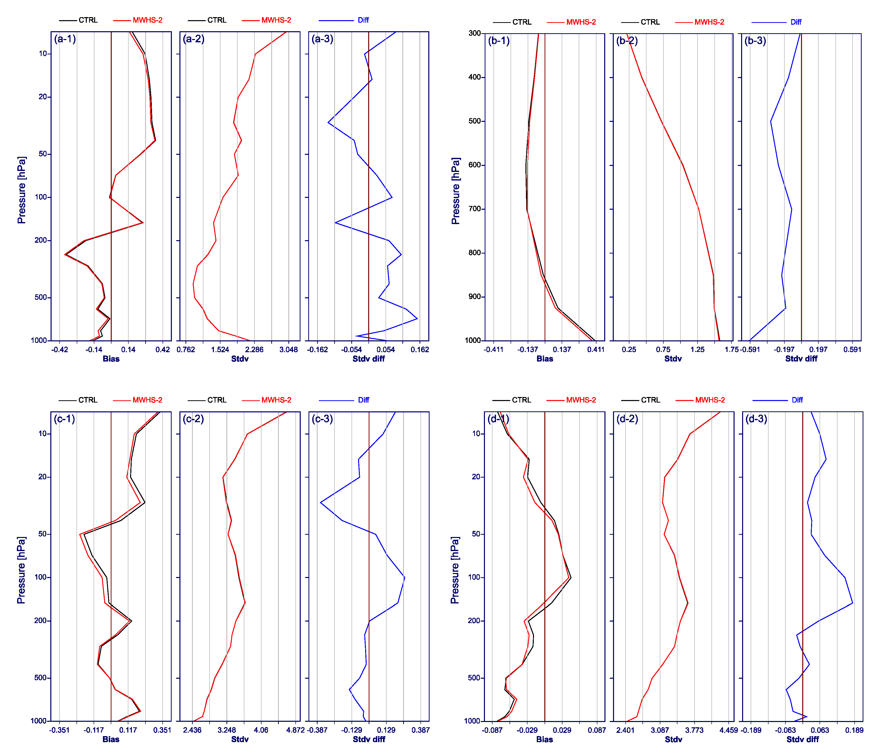
4.3. Impacts of MWHS-2 on Analyses

The main contribution of MWHS-2 assimilation is the changes to the analyses, followed by the impact on short-range and medium-range forecasts. The vertical structure of the zonal-mean yearly mean of specific humidity analysis covering 1 August 2016 to 31 August 2017 is explored. Figure 4a,b show the structures for the “MWHS-2” experiment and ERA5 reanalysis, respectively. It can be seen that specific humidity varies dramatically with latitude, with the highest value near the equator and decreases toward the poles. Vertically, specific humidity decreases from the bottom (up to 18 g/kg near the equator) to the top of the atmosphere. There is little water vapor in the atmosphere higher than 300 hPa. Figure 4c shows the yearly mean difference between “CTRL” and ERA5. It can be seen that the specific humidity of the “CTRL” experiment over tropical regions is drier than ERA5 between 800 hPa to 900 hPa and 950 hPa to 1000 hPa and wetter than ERA5 above 800 hPa. Figure 4d shows the difference between experiments “MWHS-2” and “CTRL”, which reveals the main contribution of assimilating additional FY-3C MWHS-2 data. Overall, MWHS-2 DA produces obvious wetter analyses below 700 hPa between 20° S and 20° N with the value up to 0.12 g/kg at 850 hPa near the equator and drier analyses above 700 hPa.

To investigate the contribution to geographical distribution, the horizontal yearly mean differences between “MWHS-2” and “CTRL” are plotted, as shown in Figure 5a at 850 hPa and Figure 5b at 700 hPa. The assimilation of MWHS-2 observations causes the analysis to be obviously moister in tropical oceans at 850 hPa with the increased highest value up to 0.2 g/kg, and drier in most regions at 700 hPa.

4.4. Impacts of MWHS-2 on 6-h Forecasts

It was pointed out that by assimilating MWHS-2 183 GHz channels, the background departures from water vapor channels of other satellite instruments (e.g., AIRS, IASI, HIRS, ATMS, MHS and SSMI/S) were reduced by around 0.5% in the ECMWF NWP system [6]. In this study, we explore the changes of the 6-h forecasts (background) against radiosonde temperature, specific humidity, meridional wind, and zonal wind observations directly. The mean and Stdv of (O−B) for the two experiments, along with the Stdv difference in percentage between the two experiments calculated as 100 × (“MWHS-2” Stdv−“CTRL” Stdv)/(“CTRL” Stdv), are shown for the global average over the period from August 1, 2016 to August 31, 2017 (Figure 6). For the temperature profile, it can be seen that the mean of O−B (bias) for the “MWHS-2” experiment is closer to zero than in “CTRL” for the atmosphere above 50 hPa (Figure 6a-1). The vertical patterns of temperature Stdv for the two experiments are very similar (Figure 6a-2), with reductions up to 0.1% above 50 hPa and increments around 0.05% below 200 hPa (Figure 6a-3). For specific humidity profiles, improvements to the bias in “MWHS-2” experiments (red line) are seen in Figure 6b-1. The vertical patterns of specific humidity Stdv for the two experiments are also very similar, as shown in Figure 6b-2. Significant reductions over the whole vertical profile are seen in Figure 6b-3, with values up to 0.6%, indicating that the assimilation of MWHS-2 observations causes the 6-h forecast to fit more closely to radiosonde observations. The changes of meridional wind (Figure 6c) and zonal wind (Figure 6d) are also analyzed. Improvements in lower levels (below 200 hPa) are seen, as shown in Figure 6c-3. Overall, the assimilation of MWHS-2 observations makes the 6-h specific humidity forecasts fit notably closer to radiosonde observations between 500 hPa and 700 hPa and also below 850 hPa.

To further investigate the added value of MWHS-2 DA, the Stdv of specific humidity 6-h forecast errors against ERA5 reanalysis are calculated for both experiments using their 6 hourly results. The zonal-mean vertical-meridional cross-section of the Stdv for the “CTRL” experiment is shown in Figure 7a, and the Stdv difference between “MWHS-2” and “CTRL” is shown in Figure 7b. It can be seen that the highest errors up to 1.8 g/kg are located at 850 hPa near 10° S and at 925 hPa near 33° N. An obvious error reduction is shown in Figure 7b, indicating that MWHS-2 DA improves the 6-h forecast scores compared with ERA5 reanalysis. The error reduction can be up to 0.04 g/kg in tropical regions.

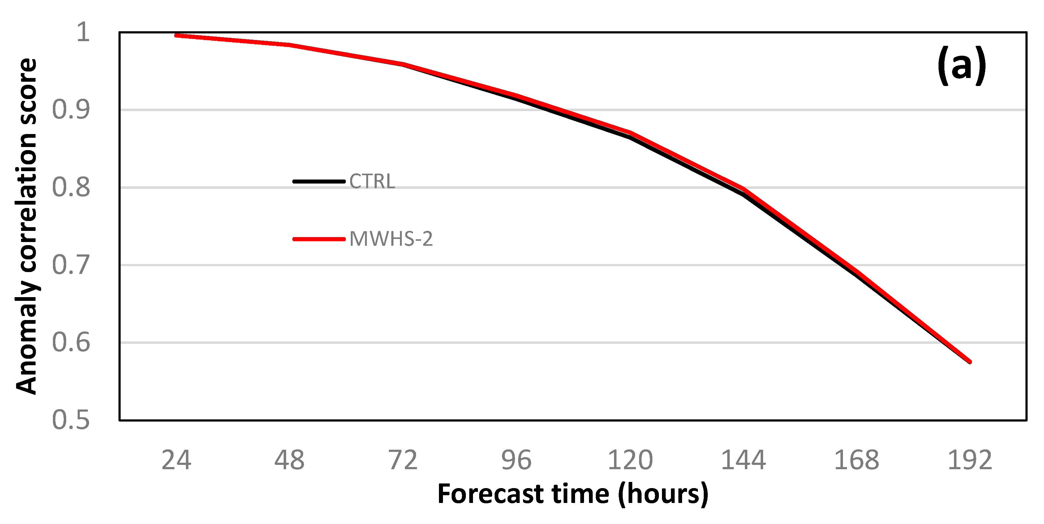
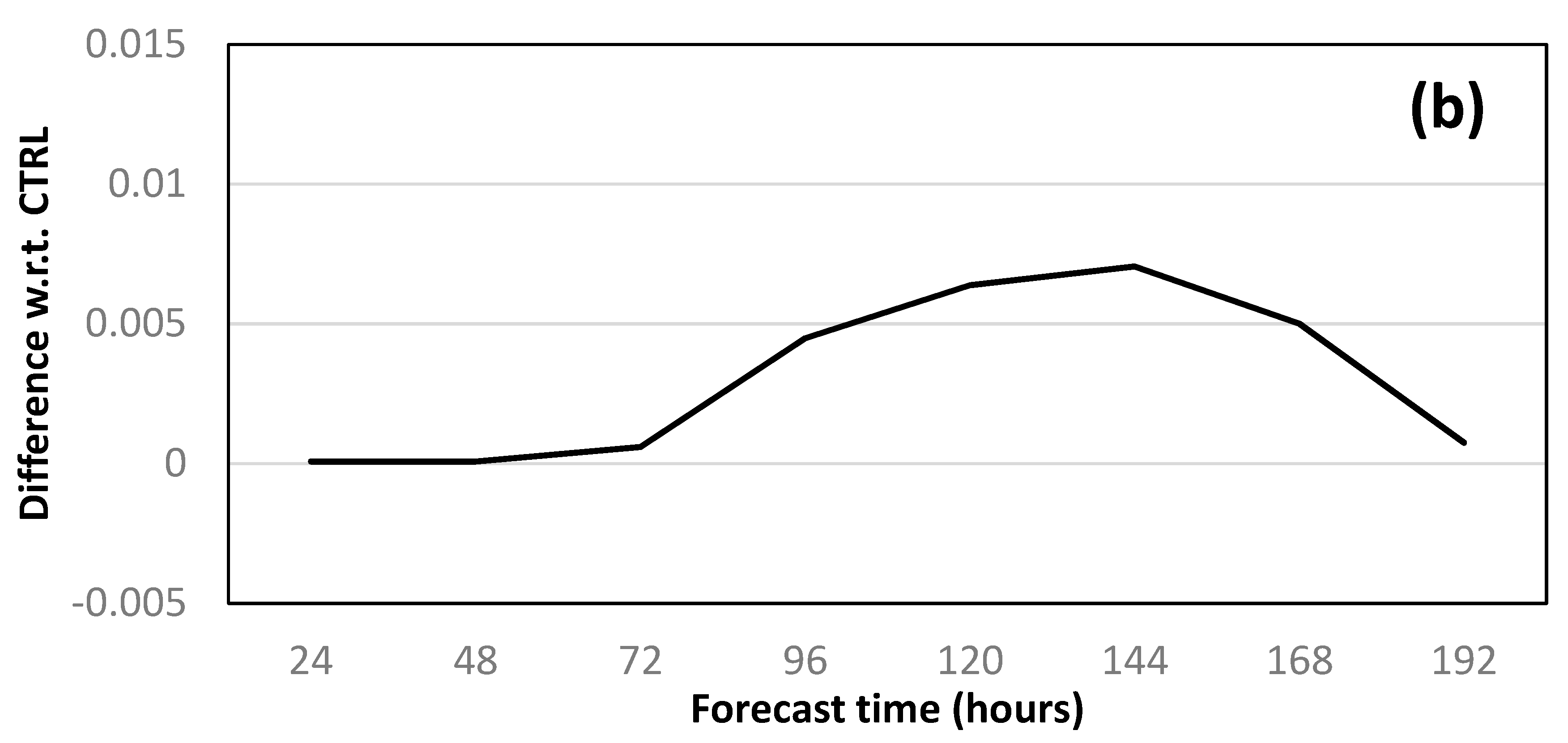
4.5. Impacts of MWHS-2 on Medium-Range Forecasts

Eight-day forecasts initialized at 00z from 1–5 August 2016 using the analyses from the two experiments are also conducted, to investigate the impact on medium-range forecasts of assimilating additional MWHS-2 data. Figure 8a shows the global average of 500-hPa geopotential height anomaly correlation scores by forecast time from 24 h to 192 h for “CTRL” (blue line) and “MWHS-2” (red line), while Figure 8b shows the difference of scores between the two experiments (MWHS-2−CTRL). It can be seen that the forecast scores decrease with increasing forecast lead-time. The MWHS-2 experiment has slightly higher forecast scores through forecast times from 72 h to 192 h. The score increases by around 0.006 for the 144-h forecast. This result suggests that assimilating MWHS-2 observations brings benefits to 3–8-day forecasts.

5. Discussion

Long-term cycling data assimilation experiments show that the bias of MWHS-2 observations is stable, except for occasional sudden jumps. Fortunately, the bias seems to be global offsets (e.g., Figure 1e) and can be effectively removed by VarBC. Apart from the bias jumps, the Stdv of O−B for MWHS-2 is comparable to equivalent channels from MHS and ATMS, which are widely used in NWP. It is found that the addition of MWHS-2 DA makes the specific humidity analysis field wetter below 700 hPa and drier above 700 hPa between 20° S and 20° N, and then leads the 6-h forecasts to fit more closely to radiosonde observations with a reduction of 0.55–1% for the O−B Stdv of specific humidity, as shown in Figure 6. A previous study performed in the UK Met Office global model shows that MWHS-2 DA improves the model background fit to observations of independent instruments by up to 1% [7]. Moreover, MWHS-2 DA reduces 6-h specific humidity forecast error by 0.02–0.04 g/kg in tropical regions between 500 hPa and 900 hPa, as shown in Figure 7, compared with independent reanalysis products (ERA5). Improved humidity analysis may cause changes of precipitation, and consequently affects the dynamical fields forecasts, e.g., through the latent heat release. Thus, medium-range forecast experiments are performed. The Results show that, MWHS-2 DA slightly increases the 500-hPa geopotential height anomaly correlation scores from 72-h to 192-h forecasts with the highest increments around 0.006 for the 144-h forecast. Similar research shows that the improved humidity analysis produced positive dynamical impact on 10-day forecast, especially in tropics [23]. It is worth noting that there is already a lot of satellite observations in the global observing system. This may limit the contribution of FY-3C MWHS-2 DA to improving forecast scores.

6. Conclusions

FY-3C MWHS-2 radiance observations are introduced to the GSI global analysis system with newly developed preprocessing and QC procedures. The VarBC scheme within GSI performs very well to remove the bias of MWHS-2 radiance observations. MWHS-2 has similar data quality to MHS and ATMS. Cycling DA experiments covering more than one year demonstrate that assimilating MWHS-2 makes the 6-h forecasts fit more closely to radiosonde observations and reduces the 6-h specific humidity forecast error against ERA5. MWHS-2 DA may also benefit from the improvement on the 500-hPa geopotential height anomaly correlation scores of 3–8 day forecasts.

References

1. Cucurull, L.; Anthes, R. Impact of infrared, microwave, and radio occultation satellite observations on operational numerical weather prediction. Mon. Weather Rev. 2014, 142, 4164–4186. [Google Scholar] [CrossRef] [Green Version]
2. Li, J.; Qin, Z.; Liu, G. A new generation of Chinese FY-3C microwave sounding measurements and the initial assessments of its observations. Int. J. Remote Sens. 2016, 37, 4035–4058. [Google Scholar] [CrossRef]
3. Lu, Q.; Bell, W.; Bauer, P.; Bormann, N.; Peubey, C. An evaluation of FY-3A satellite data for numerical weather prediction. Quart. J. R. Meteor. Soc. 2011, 137, 1298–1311. [Google Scholar] [CrossRef]
4. Chen, K.; English, S.; Bormann, N.; Zhu, J. Assessment of FY-3A and FY-3B MWHS observations. Weather Forecast. 2015, 30, 1280–1290. [Google Scholar] [CrossRef]
5. Lawrence, H.; Carminati, F.; Bell, W.; Bormann, N.; Newman, S.; Atkinson, N.; Geer, A.J.; Migliorini, S.; Lu, Q.; Chen, K. An evaluation of FY-3C MWRI and Assessment of the Long-Term Quality of FY- 3C MWHS-2 at ECMWF and the Met Office; Techical Memorandum No. 798; European Centre for Medium-Range Weather Forecasts: Reading, UK, 2017; pp. 1–26. [Google Scholar] [CrossRef]
6. Lawrence, H.; Bormann, N.; Geer, A.J.; Lu, Q.; English, S.J. Evaluation and assimilation of the microwave sounder MWHS-2 onboard FY-3C in the ECMWF numerical weather prediction system. IEEE Trans. Geosci. Remote Sens. 2018, 56, 3333–3349. [Google Scholar] [CrossRef]
7. Carminati, F.; Candy, B.; Bell, W.; Atkinson, N. Assessment and assimilation of FY-3 humidity sounders and imager in the UK Met Office global model. Adv. Atmos. Sci. 2018, 35, 942–954. [Google Scholar] [CrossRef]
8. Xu, D.; Min, J.; Shen, F.; Ban, J.; Chen, P. Assimilation of MWHS radiance data from the FY-3B satellite with the WRF Hybrid-3DVAR system for the forecasting of binary typhoons. J. Adv. Model. Earth Syst. 2016, 8, 1014–1028. [Google Scholar] [CrossRef] [Green Version]
9. Hersbach, H.; Bell, B.; Berrisford, P.; Hirahara, S.; Horányi, A.; Muñoz-Sabater, J.; Nicolas, J.; Peubey, C.; Radu, R.; Schepers, D.; et al. The ERA5 global reanalysis. Quart. J. R. Meteor. Soc. 2020, 1–51. [Google Scholar] [CrossRef]
10. Liu, Z.Q.; Shi, C.X.; Zhou, Z.J.; Jiang, L.P.; Liang, X.; Zhang, T.; Liao, J.; Liu, J.W.; Wang, M.Y.; Yao, S. CMA global reanalysis (CRA-40): Status and plans. In Proceedings of the Proc. 5th International Conference on Reanalysis, Rome, Italy, 13–17 November 2017. [Google Scholar]
11. Zou, X.; Lin, L.; Weng, F. Absolute calibration of ATMS upper level temperature sounding channels using GPS RO observations. IEEE Trans. Geosci. Remote Sens. 2014, 52, 1397–1406. [Google Scholar] [CrossRef]
12. He, J.; Zhang, S.Z.; Wang, Z. Advanced microwave atmospheric sounder (AMAS) channel specifications and T/V calibration results on FY-3C satellite. IEEE Trans. Geosci. Remote Sens. 2015, 53, 481–493. [Google Scholar] [CrossRef]
13. Bormann, N.; Fouilloux, A.; Bell, W. Evaluation and assimilation of ATMS data in the ECMWF system. J. Geophys. Res. Atmos. 2013, 118, 912–970. [Google Scholar] [CrossRef]
14. Rabier, F.; Thépaut, J.-N.; Courtier, P. Extended assimilation and forecast experiments with a four-dimensional variational assimilation system. Quart. J. R. Meteor. Soc. 1998, 124, 1861–1887. [Google Scholar] [CrossRef]
15. Lawless, A.S. A note on the analysis error associated with 3D-FGAT. Quart. J. R. Meteor. Soc. 2010, 136, 1094–1098. [Google Scholar] [CrossRef]
16. Derber, J.C. A variational continuous assimilation technique. Mon. Weather Rev. 1989, 117, 2437–2446. [Google Scholar] [CrossRef]
17. Kleist, D.T.; Parrish, D.F.; Derber, J.C.; Treadon, R.; Errico, R.M.; Yang, R. Improving incremental balance in the GSI 3DVAR analysis system. Mon. Weather Rev. 2009, 137, 1046–1060. [Google Scholar] [CrossRef]
18. Han, Y.; Delst, P.; Liu, Q.; Weng, F.; Yan, B.; Treadon, R.; Derber, J. JCSDA Community Radiative Transfer Model (CRTM)—Version 1, NOAA. Tech. Rep. 2006, 122, 33. [Google Scholar]
19. Liu, Q.; Weng, F. Advanced doubling-adding method for radiative transfer in planetary atmosphere. J. Atmos. Sci. 2016, 63, 3459–3465. [Google Scholar] [CrossRef]
20. Sela, J. The derivation of the sigma pressure hybrid coordinates semi-Lagrangian model equations for the GFS. NCEP Off. Note 462 2010, 462, 31. [Google Scholar]
21. Zou, X.; Qin, Z.; Weng, F. Impacts from assimilation of one data stream of AMSU-A and MHS radiances on quantitative precipitation forecasts. Quart. J. R. Meteor. Soc. 2017, 143, 731–743. [Google Scholar] [CrossRef]
22. Zhu, Y.; Derber, J.; Collard, A.; Dee, D.; Treadon, R.; Gayno, G.; Jung, J.A. Enhanced radiance bias correction in the national centers for environmental prediction’s gridpoint statistical interpolation data assimilation system. Quart. J. R. Meteor. Soc. 2014, 140, 1479–1492. [Google Scholar] [CrossRef]
23. Andersson, E.; Hólm, E.; Bauer, P.; Beljaars, A.; Kelly, G.A.; McNally, A.P.; Simmons, A.J.; Thépaut, J.-N.; Tompkins, A.M. Analysis and forecast impact of the main humidity observing systems. Quart. J. R. Meteor. Soc. 2007, 133, 1473–1485. [Google Scholar] [CrossRef]
Figure 1. Mean of O−B before (red line) and after (blue line) variational bias correction (VarBC), and the O−B for MWHS-2 channel 11 (a), channel 13 (b), channel 15 (c), and channel 3 (d). (e) is the global offset coefficient for channel 3 used in the VarBC scheme.
Remotesensing 12 02511 g001aRemotesensing 12 02511 g001b
Figure 2. Scatterplots of observations from Feng-Yun-3C (FY-3C) MWHS-2 channel 15 (a,b), Suomi National Polar-orbiting Partnership (SNPP) ATMS channel 18 (c,d) and MetOP-B MHS (e,f) passing (blue points) and rejected by (red points) quality control (QC) versus the equivalent brightness temperature calculated from 6-h forecast (a,c,e) and analysis (b,d,f) in the “MWHS-2” experiment. The time period of observations is from 21Z 31 July 2016 to 03Z 2 August 2016.
Remotesensing 12 02511 g002
Figure 3. Time series of the Stdv of O−B (a), O−A (b), and O−B minus O−A (c), as well as the number of observations (d) for MWHS-2 channel 13 (red line), SNPP ATMS channel 20 (blue line) and MetOP-B MHS channel 4 (black line).
Remotesensing 12 02511 g003aRemotesensing 12 02511 g003b
Figure 4. Zonal-mean cross-section of yearly mean (from August 1, 2016 to August 31, 2017) specific humidity analysis for the “MWHS-2” experiment (a) and (ERA5) (b) and the differences between “CTRL” and ERA5 (c) and also the differences between “MWHS-2” and “CTRL” (d).
Remotesensing 12 02511 g004
Figure 5. Geographical distribution of yearly mean specific humidity differences (g/kg) between the analysis fields in the “MWHS-2” and “CTRL” experiments at 850 hPa (a) and 700 hPa (b).
Remotesensing 12 02511 g005
Figure 6. Mean, Stdv, and Stdv differences (left-to-right for each subplot) of radiosonde observed (a) temperature (K), (b) specific humidity (g/kg), (c) meridional wind (m/s), and (d) zonal wind (m/s) minus 6-h forecasts for the “CTRL” (black line) and “MWHS-2” (red line) experiments, averaged globally from August 1, 2016 to August 31, 2017. The Stdv differences (blue line) are calculated by 100 × (“MWHS-2” Stdv−“CTRL” Stdv)/(“CTRL” Stdv), indicating the percentage change of Stdv from assimilating MWHS-2 observations.
Remotesensing 12 02511 g006
Figure 7. (a) Zonal-mean cross-section of the standard deviation of 6-h specific humidity forecasts errors against ERA5 reanalysis for the “CTRL” experiment in August 2016. (b) the standard deviation difference between “MWHS-2” and “CTRL”.
Remotesensing 12 02511 g007
Figure 8. (a) Global average of 500-hPa geopotential height anomaly correlation against forecast lead-time for the CTRL (blue line) and MWHS-2 (red line) experiments initialized at 00Z from August 1–5, 2016. (b) The difference between the experiments (MWHS-2 minus CTRL).
Remotesensing 12 02511 g008aRemotesensing 12 02511 g008b