Article

Estimating Forest Stock Volume in Hunan Province, China, by Integrating In Situ Plot Data, Sentinel-2 Images, and Linear and Machine Learning Regression Models

1
College of Forestry, Beijing Forestry University, Beijing 100083, China
2
Academy of Inventory and Planning, National Forestry and Grassland Administration, Beijing 100714, China
3
College of Environment and Planning, Ministry of Education Key Laboratory of Geospatial Technology for Middle and Lower Yellow River Regions, Henan Collaborative Innovation Center of Urban-Rural Coordinated Development, Henan University, Kaifeng 475004, China
4
Department of Geosciences, Mississippi State University, Mississippi State, MS 39762, USA
5
School of Resource and Environmental Sciences, Wuhan University, Wuhan 430079, China
6
Research Station of Ecology, Guizhou Academy of Forestry, Guiyang 550000, China
7
Geography Information and Tourism College, Chuzhou University, Chuzhou 239000, China
8
Department of Microbiology and Plant Biology, University of Oklahoma, Norman, OK 73019, USA
*
Author to whom correspondence should be addressed.
Remote Sens. 2020, 12(1), 186; https://doi.org/10.3390/rs12010186
Submission received: 20 November 2019 / Revised: 31 December 2019 / Accepted: 2 January 2020 / Published: 4 January 2020
(This article belongs to the Section Forest Remote Sensing)

Abstract

:
The forest stock volume (FSV) is one of the key indicators in forestry resource assessments on local, regional, and national scales. To date, scaling up in situ plot-scale measurements across landscapes is still a great challenge in the estimation of FSVs. In this study, Sentinel-2 imagery, the Google Earth Engine (GEE) cloud computing platform, three base station joint differential positioning technology (TBSJDPT), and three algorithms were used to build an FSV model for forests located in Hunan Province, southern China. The GEE cloud computing platform was used to extract the imagery variables from the Sentinel-2 imagery pixels. The TBSJDPT was put forward and used to provide high-precision positions of the sample plot data. The random forests (RF), support vector regression (SVR), and multiple linear regression (MLR) algorithms were used to estimate the FSV. For each pixel, 24 variables were extracted from the Sentinel-2 images taken in 2017 and 2018. The RF model performed the best in both the training phase (i.e., R2 = 0.91, RMSE = 35.13 m3 ha−1, n = 321) and in the test phase (i.e., R2 = 0.58, RMSE = 65.03 m3 ha−1, and n = 138). This model was followed by the SVR model (R2 = 0.54, RMSE = 65.60 m3 ha−1, n = 321 in training; R2 = 0.54, RMSE = 66.00 m3 ha−1, n = 138 in testing), which was slightly better than the MLR model (R2 = 0.38, RMSE = 75.74 m3 ha−1, and n = 321 in training; R2 = 0.49, RMSE = 70.22 m3 ha−1, and n = 138 in testing) in both the training phase and test phase. The best predictive band was Red-Edge 1 (B5), which performed well both in the machine learning methods and in the MLR method. The Blue band (B2), Green band (B3), Red band (B4), SWIR2 band (B12), and vegetation indices (TCW, NDVI_B5, and TCB) were used in the machine learning models, and only one vegetation index (MSI) was used in the MLR model. We mapped the FSV distribution in Hunan Province (3.50 × 10⁸ m3) based on the RF model; it reached a total accuracy of 63.87% compared with the official forest report in 2017 (5.48 × 10⁸ m3). The results from this study will help develop and improve satellite-based methods to estimate FSVs on local, regional and national scales.

Graphical Abstract

1. Introduction

The forest stock volume (FSV, m3 ha−1) is the sum of the stem volumes of all the living trees per unit area, and is one of key forest variables for forest resources management and assessments on local, region and country scales [1]. FSVs have a strong relationship with the aboveground biomass (AGB) and carbon stocks [2]. To understand the spatial distribution of carbon in forests and to derive predictions for monitoring carbon stock trends, the FSV must be quantified [3]. Traditionally, the FSV is estimated by sampling several plots, which involves substantial manpower, materials, and financial resources [4]. With the development of remote sensing technology, particularly the Landsat series since 1972, satellite imagery has played an important role in forest inventory. Various studies have been performed to estimate the forest variables using low spatial resolution (LSR, LSR ≥ 30 m), moderate spatial resolution (MSR, 5 m < MSR < 30 m), and high spatial resolution (HSR, HSR ≤ 5 m) [5] data obtained by different optical sensors (e.g., Landsat [6,7,8,9,10,11], MODIS [12,13,14,15,16], SPOT [17,18,19,20], Quickbird [21,22,23,24,25,26], RapidEye [27,28,29,30]), microwave sensors [31,32,33,34], and light detection and ranging (LiDAR) sensors [35,36,37,38,39]. The successful applications of these technological tools have laid the foundation for the estimation of forest variables, such as the FSV, using remote sensing technology.
Two recent developments in the Earth Observation (EO) sector have increased the potential to improve the efficiency of retrieving global forest attributes. The Sentinel-2A and Sentinel-2B satellite series launched by the European Space Agency (ESA) through its Copernicus program in 2015 (S2A) and 2017 (S2B) provide nominal five-day revisit imagery across the globe [40]. The Sentinel-2 imagery includes 13 spectral bands with spatial resolutions ranging from 10–60 m [40]. One of the main purposes of the Sentinel-2 satellite series is vegetation analysis [4]. The Sentinel-2 satellite images provided by the operational environment monitoring system based on the European Copernicus program may be accessed freely. The different spatial resolution bands, the short revisit period, and the rich spectral information have made these images a popular source of remote sensing data for forestry research in recent years. For instance, Persson et al. [41] used Sentinel-2 data to classify common tree species in central Sweden, observing the highest overall accuracy, i.e., approximately 88.2%, using all the imagery bands in the final model. A study conducted by Ho’sciło et al. [42] in southern Poland affirmed that the Sentinel-2 series could accurately delineate tree species (e.g., beech, oak, birch, alder, and larch) with an overall accuracy above 85%. Similarly, Pandit et al. [43] explored the ability of Sentinel-2 images to estimate the forest biomass in Nepal; their biomass estimation model achieved an R2 = 0.81 and RMSE = 25.57 t ha−1. Zarco-Tejada et al. [44] demonstrated the potential of Sentinel-2A data to estimate the chlorophyll content in open canopy conifer forests (R2 > 0.7 for June; R2 > 0.4 for December). In the Brazilian Amazon, Lima et al. [45] performed comparative research on monitoring selective logging using Sentinel-2 and Landsat-8 OLI imagery. These authors found that Sentinel-2 data (43.2% detected) were more effective in detecting logging concessions than Landsat 8 data (35.5% detected). In Poland, Grabska et al. [46] used the Sentinel-2 time series to map forest stand species in the Carpathian Mountains and reported higher accuracy, i.e., a 5–10% improvement in overall accuracy compared with only using single date imagery. These studies demonstrate the potential of Sentinel-2 for forest vegetation monitoring.
A typical traditional remote sensing image processing approach includes data downloading and local computer processing, which render image processing computationally demanding, and also hinder the processing capability for large datasets. Regarding imagery processing, the development of cloud computing technology has been fundamentally changing traditional remote sensing image processing. The Google Earth Engine (GEE) portal is a powerful cloud-based computing platform for image processing [47,48]. The GEE archives massive, publicly-available remote sensing data, provides a programming environment, programming tools, and virtual machines for users with relatively simple code, and can process imagery data online. The GEE greatly improves the processing efficiency when using substantial amounts of remote sensing data. In recent years, the GEE was used in land cover mapping [49,50,51,52,53,54,55,56,57,58], agricultural applications [59,60,61,62,63], disaster management, and earth sciences studies [64,65,66]. This remote sensing data processing cloud platform makes the rapid processing of Sentinel-2 images covering large areas possible.
In the FSV estimation field, some studies have examined assessments of the FSVs using remote sensing. For instance, Condés et al. [67] found the model prediction of the plot-level growing stock volume using satellite images and field data to be useful; the result showed that the adj-R2 increased from 0.19 to 0.42. Using the random forests (RF) regression algorithm, Chrysafis et al. [68] estimated the FSV based on Sentinel-2 image, which provided relatively better results (R2 = 0.63, RMSE = 63.11 m3 ha−1) than Landsat-8 OLI images (R2 = 0.62, RMSE = 64.40 m3 ha−1). However, some studies were conducted that combined optical images and microwave data to estimate forest variables [69,70,71]. A noteworthy study was conducted by Mauya et al. [72]; these authors assessed the multiple linear regression (MLR) models built by Sentinel-1, Sentinel-2, and ALOS PALSAR-2 images to predict the FSV, and found that Sentinel-2 images performed best with an RMSEr = 42.03% and a pseudo-R2 = 0.63. For predicting forest variables, Pham et al. showed that machine learning algorithms were likely to become more attractive in remote sensing [73]. These authors suggest that future studies using more methods, large areas, and Sentinel-2 data to predict the FSV should be conducted.
However, ground plot survey data are still indispensable for remote sensing modeling [74]. The costs of ground plot surveys have always been high, which has presented some obstacles to the estimation of the provincial FSV by remote sensing. In addition, the traditional sample location survey technology often produces serious positional deviations, which may impact the modeling accuracy of the plot data-based remote sensing estimations and predictions [75]. Thus, traditional sample location technology is also an important reason for the inaccurate matching of sample plots and pixels, which results in estimation bias. Furthermore, to the best of our knowledge, little to no research has been conducted to compare the results of the RF, support vector regression (SVR), and MLR using Sentinel-2 images to predict FSVs. In addition, no FSV mapping has been conducted in Hunan Province, and this research gap directly affects forest policy making and management. Moreover, Hunan Province is located in southern China, where cloudy conditions frequently occur; these conditions are a great challenge to mapping the FSV in Hunan Province using remote sensing images.
Hence, Sentinel-2 data on the GEE platform, 459 sample plots, and three algorithms were used in this study to achieve the following objectives: (1) to identify and select the most important variables of the Sentinel-2 images for FSV estimation using plot-level tree measurements from a large number of in situ sites in Hunan Province, southern China, where forest species and stand structures are complex; (2) to assess and understand the performance of machine learning algorithms and the typical MLR models for FSV estimation; and (3) to map the FSV in Hunan Province. This study will help move towards the overall goal of developing and improving GEE-based remote sensing approaches to estimate the FSV on local, regional and national scales.

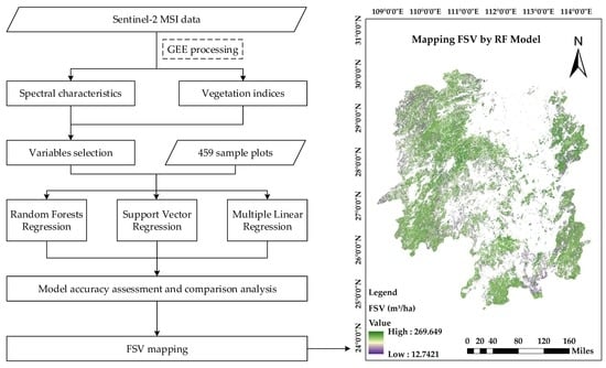
2. Materials and Methods

2.1. Study Area

The study was conducted in Hunan Province, covering an estimated area of 211,854.69 km2. This area is a transition zone between the middle and lower ridges of the Yangtze and Xiangjiang river basins and the Yungui Plateau. The area has a subtropical monsoon climate with four distinct seasons. The annual precipitation ranges from 1200 to 1700 mm, and the mean annual temperatures vary between 16 °C and 18 °C [76]. These favorable climatic conditions make Hunan Province one of the major forest areas in China. In the study area, the Global PALSAR-2/PALSAR Forest/Non-Forest Map product was used as ancillary data to determine the forest areas and show the distribution of the training plots and test plots (Figure 1).

2.2. In situ Sample Plot Data Collection

Based on the historic forest survey data, 10 forest types were chosen for this study. The forest types were first analyzed using the 8th National Forest Inventory (NFI) data, and then the top seven tree species were selected according to the stock volume. These species included Cunninghamia lanceolata, Pinus massoniana, Quercus sp., Pinus elliottii, Populus sp., Cinnamomum camphora, and Cupressus funebris. In addition, three mixed forest types were selected, including broad-leaved mixed forests, coniferous and broad-leaved mixed forests, and coniferous mixed forests. These ten types account for over 98% of the total FSV in Hunan (Table 1).
A total of 15 survey levels were generated in each forest type. Each forest survey type was further divided into five tree height levels and three canopy density degrees (0.2–0.39, 0.4–0.69, and 0.7–1.0). At each surveyed level, four sample plots were designed and investigated. Finally, 459 useful circle sample plots with a diameter of 30 m were obtained from 15 October 2017, to 30 April 2018. The tree heights (measured by a VERTEX LASER VL5 manufactured in Haglof, Sweden) and diameters at breast height (DBHs) were measured for all individual trees (measured by a caliper with a DBH greater than 5 cm) in the circle sample plot. TBSJDPT (Figure 2) was put forward and used to locate the sample plot center and the individual trees [39].
To match the pixels of the Sentinel-2 imagery, the sample plot data were resampled using the ArcGIS 10.2.2 software (Esri, Redlands, CA, USA). By using the center position of each sample plot, the 25 m × 25 m area sample plots were generated by using the ArcTools “Buffer and Feature Envelope To Polygon”. The generated shapefile was then used to extract the trees in the sample plot. Using the formula built by Hunan Forestry Industry Survey and Design Research Institute, we calculated the FSV of each tree, summed it to obtain the FSV of the sample plots, and then scaled it up to obtain the FSV per hectare (Table 2). In addition, we used the “boxcox” function in the R software to transform the FSV data to a normal distribution (f(y) = yλ) [77].

2.3. Sentinel-2 Images Preprocessing and Variable Calculation

To obtain a temporal match between the investigated sample plot data and the satellite data for the whole of Hunan Province, the GEE filtering options were used to select the Sentinel-2 Level-1C (TOA, top-of-atmosphere) satellite images between 1 May 2017, and 31 October 2017, and between 1 May 2018, and 31 October 2018. The Level-1C product is an ortho-image in UTM/WGS84 projection. Level-1C processing includes radiometric and geometric corrections, including orthorectification-Digital Elevation Model (DEM, processed from Shuttle Radar Topography Mission 90 m Digital Elevation Data Version 4) to project the images in cartographic geometry. Per-pixel radiometric measurements are provided in TOA reflectances along with the parameters to transform them into radiances, and spatial registration was processed on a global reference system with subpixel accuracy. In addition, the Level-1C products provide a bitmask band (QA60) to show cloud information. More details about the Level-1C products could be found in the Sentinel-2 User Handbook [79]. The Level-1C product stored in the GEE has been shown to be suitable for direct use for land mapping by Hird et al. [57]. The cloud mask steps were processed in this study. The QA60 band was first used to identify and mask out the flagged cloud and cirrus pixels. Then, the two thresholds of Band 1 ≥ 0.15 and Band 2 ≤ 0.25 were used to mask the remaining clouds and noise [57,80]. A total of 3150 images covering the entire study area over the study period were processed. After that, the Level-1C TOA reflectance data were resampled with a resolution of 25 m to match the spatial resolution of survey plots. Then, we extracted the median values of the characteristic variables using the GEE cloud computing platform [58]. The characteristic variables included the multispectral bands (B2, B3, B4, B5, B6, B7, B8, B8A, B10, B11, and B12) and the vegetation indices selected according to the research of Astola et al. [4], Wittke et al. [81], and Xia et al. [82]. The vegetation indices were calculated as follows (Table 3).

2.4. Selection of Relevant Variables for FSV Estimation

For the MLR method, the “redun” function was used to avoid collinearity. The parameter R2 was set to 0.9. Then, the variables were further filtered based on their significance (i.e., P < 0.05) and variance inflation factor (i.e., VIF > 10). For the machine learning methods, in order to obtain the best fit model, the selection of the relevant variables for the FSV estimation was carried out using the “variable selection using random forests” (VSURF) package [83]. All the extracted data were analyzed in order to obtain the variable importance measures (VIM) based on the VSURF package in the R 3.5.3 software (R Core Team, Vienna, Austria). Importance type 1 represents the percentage increase in the mean square error (PercentIncMSE), and importance type 2 represents the increase in the NodePurity (IncNodePurity); each had the ability to evaluate the importance of variables [83]. The selected variables were then used in RF modeling and SVR modeling.

2.5. Statistical Models for Estimating the FSV

The MLR is a statistical technique that uses several explanatory variables (independent variables) to predict the outcome of a response variable (dependent variable). The MLR is a widely used method to construct regression models for various applications [72,84,85,86,87]. The goal of the MLR is to model the linear relationship between the explanatory (independent) variables and response (dependent) variable (FSV). The formula for the MLR is
y = a + b 1 x 1 + b 2 x 2 + b 3 x 3 + + b i x i + ε
where i is the number of variables, y is the dependent variable, xi is the independent variable, a is the intercept, bi is the slope coefficient for the explanatory variable, and ε is the error term of the model.
The SVR maps the output data to the high-dimensional feature space by defining the kernel function and constructs an optimal classification hyperplane in this space. The SVR can be regarded as a linear algorithm in high-dimensional space [88]. The SVR has been proven to be a popular method for regression modeling [89,90,91,92]. In this study, it was constructed using the following SVR function from the training process:
FSV = i = 1 n α i k ( x i ; x ) + b
where k ( x i ; x ) is the kernel function, α i is the Lagrange multiplier, x i is the training vector, and b is the bias term in the regression.
Using the e1071 package in the R 3.5.3 software, the parameters of the SVR were optimized and cross-validated. The radial basis function (RBF) kernel was selected following previous studies [71,93]. Then, the best regression model was optimized by the tune function (the SVM-type is eps-regression, the SVM-Kernel is the radial, cost is set as 2c (c is 2-9 sequence with an interval of 1), epsilon is set as a 0-1 sequence with an interval 0.01, and gamma is default).
The RF is a decision tree algorithm and an effective machine learning model for predicting a forest of variables. Based on its powerful modeling capabilities, the RF regression has been widely used in scientific research [94,95,96,97,98,99]. The principle of the RF algorithm is to use the bootstrap method to randomly extract multiple samples to generate a group of regression trees (ntree) from the original sample population. To build each tree, a randomly-chosen subset of predictors is used at each splitting node (mtry) by the RF, and there is no need to prune each tree grown. For each tree grown, a procedure named the “out-of-bag” (OOB) error was used to independently build each tree based on the training data. The variable importance (VI) and OOB error were calculated by the RF algorithm [100].
The OOB error can be estimated as follows:
O O B e r r o r =   1 n i = 1 n ( y i y ^ i ) 2
where y i is the measured FSV, y ^ i is the predicted FSV, and n is the total number of OOB samples.
After selecting the variables, the number of grown trees (ntree) and the number of variables (mtry) at the time of node splitting were determined using the minimum mean square error as the criterion. First, the RF model’s ntree parameter was set to 500, and the mtry parameter was set to the total number of variables. Then, the mean square error was used to determine the best number of variables (mtry) and the best number of trees (ntree). After calculating the best parameters, the RF regression model was established and tested. In our three models, 70% of the total samples were used for training samples, and 30% of the overall samples were used for testing.
Two statistical indicators were selected to evaluate the performance of the MLR, SVR, and RF models [88,101]. The coefficient of determination (R2, Equation (4)) is the proportion of the variance in the dependent variable that can be explained by the independent variables. The root mean square error (RMSE, Equation (5)) is the standard deviation of the residuals, which is the difference between the surveyed data and the fitted model.
R 2 = 1 i = 1 n ( y i y ^ i ) 2 i = 1 n ( y i y ¯ ) 2
RMSE = i = 1 n ( y i y ^ i ) 2 n
where y i is the measured FSV, y ¯ is the mean measured FSV, y ^ i is the predicted FSV, i is the same index, and n is the sample plot number.

3. Results

3.1. Characteristics of the in Situ FSV Data

For this study, 321 out of the 459 total sample plots (70%) were used as the training data, and 138 out of the 459 total sample plots (30%) were used as the test data. Table 4 lists the summarized statistics of the plot-level training data and test data. For the training data, the minimum FSV per hectare was only 1.42 m3, and the maximum FSV per hectare was 577.49 m3. For the test data, the FSV per hectare ranged from 4.25 m3 to 450.11 m3. These large data ranges were the reason for the large variances in the training and test data. For the training data and test data before transformation, it is clear that the training data and test data did not follow a normal distribution (Figure 3, the green histograms with red curves). A λ = 0.3030303 was calculated and used to transform the training data and test data, and it is clear that the data were transformed into an approximately normal distribution (Figure 3, the red histograms with green curves).

3.2. Major Variables Related to the FSV Data

Figure 4 shows the results of the numbers of selected variables using the RF algorithms provided by the VSURF package. First, no variables were eliminated based on the VI mean and VI standard deviations. Based on the OOB error, eight variables were selected: B2, B3, B4, B5, B12, TCW, TCB, and NDVI_B5. The PercentIncMSE (percent increase in the mean square error) and IncNodePurity (increase in the NodePurity) estimated from the RF OOB data were used to rank all predictor variables according to their abilities to estimate the FSV; the higher the value, the more important the variable (Figure 5).
For the MLR algorithm, 14 out of the 24 variables were eliminated by the “redun” function to avoid multicollinearity; these eliminated variables were NDVI_B8, EVI2, SAVI, NDVI_B7, B7, B8A, TCB, NDVI_B6, B6, B3, B11, TCG, NDVI_B8A, and B4. The remaining variables were reselectedusing the P significance in linear modeling. Finally, B5 and MSI were selected for the MLR model.

3.3. Optimal Regression Model for the RF, SVR, and MLR

For the RF model, before selecting the best RF regression model, the mtry and ntree parameters must first be determined. Based on the number of selected variables, an error rate loop algorithm was used to calculate the smallest error rate. In Figure 6a, it is clear that mtry = 5 resulted in the smallest error rate. In Figure 6b, ntree = 257 was determined to be the best parameter.
In the SVR algorithm, 909 models were trained. The best model that was selected had cost = 8, gamma = 0.125, and epsilon = 0.68. Then, the best SVR regression was used to build the regression model for the FSV prediction. In the MLR algorithm, the results of the MLR model are shown in Table 5.
A basic hypothesis test was made for the linear model (Figure 7). In Figure 7, the top left graph, the residuals versus the fitted values, was used to test the linearity assumptions. The scatter points were concentrated near a straight line, which indicated that the linear relationship was good. The top right graph was a normal Q-Q plot, which was used to test the normality. The scatter points were mainly concentrated along the straight line, which indicated that the residual normality was good. The bottom left graph was the scale-location graph, which was used to test the homoscedasticity. The points were randomly distributed around the curve, which indicated that the homoscedasticity assumption was accepted. The bottom right graph used the residual and leverage to determine the outliers, and no high leverage points or strong influence points were found.

3.4. Comparison of the Predicted FSV Estimates among the Three Models (MLR, SVR, and RF)

In the training phase, the MLR model had the worst performance with the smallest R2 = 0.38 and highest RMSE = 75.74 m3 ha−1 (Figure 8a). This model was followed by the SVR model with an R2 = 0.54 and RMSE = 65.60 m3 ha−1 (Figure 8c). The best performance among the three algorithms was that of the RF model, which had the highest R2 = 0.91 and smallest RMSE = 35.13 m3 ha−1 (Figure 8e). In the test phase, it was clear that the RF model also performed the best among the three kinds of models (R2 = 0.58, RMSE = 65.03 m3 ha−1) (Figure 8f); the next best was the SVR model, with an R2 = 0.54 and RMSE = 66.00 m3 ha−1 (Figure 8d); the MLR model performed the worst, with the smallest R2 = 0.49 and highest RMSE = 70.22 m3 ha−1 (Figure 8b).

3.5. Modeling Results Comparison between Selected Variables and all Variables

Table 6 shows the modeling performance of all variables and selected variables under the machine learning methods. In the training phase, the result of the RF model with all variables (e.g., R2.training = 0.92, RMSE = 34.83 m3 ha−1) is basically the same as that of the RF model with the selected variables (e.g., R2.training = 0.91, RMSE = 35.13 m3 ha−1). And the results of the RF model are better than those of the SVR model with all variables (e.g., R2.training = 0.61, RMSE = 60.58 m3 ha−1) and selected variables (e.g., R2.training = 0.54, RMSE = 65.60 m3 ha−1). In the test phase, the result of the RF model with selected variables (e.g., R2.training = 0.58, RMSE = 65.03 m3 ha−1) is basically consistent with the result of the RF model with all variables (e.g., R2.training = 0.58, RMSE = 66.04 m3 ha−1). Similarly, the results of the RF model in the test phase are better than those of the SVR models with all variables (e.g., R2.training = 0.51, RMSE = 67.86 m3 ha−1) and selected variables (e.g., R2.training = 0.54, RMSE = 66.00 m3 ha−1). In the SVR model, the performance of all variables in the training phase is slightly better than that of the selected variables; and in the test phase, the performance of the selected variables is slightly better than that of the all variables.

3.6. Map of the FSV Estimation in Hunan Province in 2017

First, the Global PALSAR-2/PALSAR Forest/Non-Forest Map product was used to extract the forest area in Hunan Province. A total of 143,258,710 pixels with a 25 m spatial resolution were defined as forest areas in this product (Figure 9. left), totaling 8.95 × 10⁶ ha of forest area. Then, the selected variables and the best RF model were used to estimate the FSV in the study area. The right of Figure 9 shows that the FSV in Hunan Province ranged from 12.7421 m3 ha−1 to 269.649 m3 ha−1. The mean FSV per hectare was 39.09 m3, and the total FSV in Hunan Province was 3.50 × 10⁸ m3.

4. Discussion

The main purpose of this study was to evaluate the potential variables of the Sentinel-2 data using different algorithms to predict the FSV based on reliable field survey data, and to map the FSV for the first time in the southern province of China. The FSV is an important variable of forest management reports at the provincial and national levels. The use of free remote sensing imagery (e.g., Sentinel-2) and cloud processing platforms (e.g., GEE) to process and build prediction models for estimating and mapping the FSV is especially important in southern China. One of the reasons for this is that the area is covered by clouds many days each year, which seriously affects provincial forest mapping research that uses remote sensing images. Another reason is that the provinces of southern China are an important part of China’s forestry. Through this research, we can effectively use the Sentinel-2 data with the GEE platform and apply the RF algorithm to spatially map the FSV in Hunan Province. In addition, this approach is also an effective way to conduct forest carbon monitoring, which is sensitive and important to climate change.
Based on the spectral bands and vegetation indices extracted from Sentinel-2 data, this study has shown that B5 (Red-Edge 1) was the most important variable when estimating the FSV using both the machine learning methods and MLR method, which had been confirmed in recent studies concerning forest prediction [102] and tree species classification [103]. In the gross primary productivity field (GPP), Lin et al. found that the red-edge band was useful for estimating the GPP, and noted that the red-edge reflectance was sensitive to the leaf chlorophyll content [104]. In addition, the leaf chlorophyll content was an important forest variable. Except for B5, the modeling variables selected by the machine learning models and the MLR were not the same. However, the accuracies of the different model verification results were not very different, which shows that B5 has a substantial advantage in estimating the FSV. In the study conducted by Chrysafis et al. [68], when using the RF algorithm and Sentinel-2 images to estimate the FSV in a Mediterranean forest ecosystem, they found that the most important variable was B11 (SWIR 1), which was different from our findings in this study. Our research was consistent with a study conducted by Astola et al. [4], which showed that B5 was the most important variable with which to predict the FSV. Regarding the FSV prediction performance, we compared our R2 that measured our predictive capability with that of Astola et al. [4], who conducted research using Sentinel-2 and multilayer perceptron and regression trees to estimate the FSV; we found that our results (R2 = 0.58) were slightly better than their best results with a multilayer perceptron model (R2 = 0.56). This observation may occur because the RF algorithm usually performs better than the multilayer perceptron [71], or the sample survey data based on our advanced positioning technology improved the estimation accuracy. Regarding the variable selection in machine methods, our results also showed that the traditional vegetation indices did not perform well when estimating the FSV in this study, and Lu et al. [105] found the same trend, i.e., that the original band performed better than vegetation indices when estimating the FSV. Table 6 shows that the training and test results before and after selecting the variables of the RF modeling were basically the same, which indicated that the VSURF package was a good tool with which to select variables for RF modeling. However, Table 6 also shows that the selected variables had a certain impact on SVR modeling. This is because the VSURF package is a variable selecting tool based on the RF model, and is not fully applicable to the SVR model.
Figure 8 shows that the three algorithms have some saturation problems in the training and test phases. In the training phase, the maximum value of the RF estimation (363.63 m3 ha−1) was larger than the other two algorithms (SVR, 336.79 m3 ha−1; MLR, 308.39 m3 ha−1), and the minimum value of the RF estimation was smaller (4.97 m3 ha−1) than the other two algorithms (SVR, 6.52 m3 ha−1; MLR, 5.52 m3 ha−1). In the test phase, although the maximum value estimated by MLR (290.26 m3 ha−1) was the largest, the minimum value (7.48 m3 ha−1) was the smallest, and the data range of the RF estimated value was the largest (7.48–272.23 m3 ha−1). This indicated that the RF model was the best model with which to estimate the FSV. In addition, the RF exhibited the best performance among the three algorithms according to the R2 and RMSE. When using the RF model to predict the FSV in Hunan Province (Figure 9), we found that the smallest FSV per hectare was 12.7421 m3, which was larger than the smallest FSV measured in the field (1.42 m3 ha−1), and the largest FSV per hectare was 269.649 m3, which was smaller than the highest FSV measured (577.50 m3 ha−1). This result indicated that the RF model overestimated the low FSV values and underestimated the high FSV values, which may be due to the common saturation problem in optical remote sensing vegetation analyses [83]. The overestimation problem could be caused by the understory vegetation (e.g., shrub and grass), which typically impacts the reflectance values. The high FSV areas often have complex canopy structures, which may affect the reflectance values. A similar study by Ou et al. [106] also found this was a common problem in the estimation of the FSV or biomass using multispectral remote sensing data. However, if the forest area with a low FSV and the forest area with a high FSV reach a certain ratio, the underestimation and overestimation problems of the RF will reach a certain balance. For this reason, when using the RF to estimate the FSV over a large area, it may offset some errors caused by the defects of the model or the image data. Regarding the SVR model, Figure 8c shows two distinct trend lines consisting of points. This trend was caused by the large data volume (n = 321 in the training phase) and parameter optimization. Due to the parameter optimization, as many samples as possible were within this hyperplane; therefore, many data points were concentrated on the edge.
After mapping the FSV for the whole of Hunan Province, a statistic using the ENVI 5.3 “Quick Stats ” tool (Exelis Visual Information Solutions, Boulder, Colorado) was calculated, and the mean FSV was 39.09 m3 ha−1. For comparison, we calculated the mean FSV of Hunan Province based on the Analysis Report of Hunan Forestry Statistics Annual Report in 2017, and found that the value was 42.15 m3 ha−1 [107]. The estimation accuracy of the mean FSV reached 92.74%. However, for the sample plot data, the mean values were 121.11 and 120.53 m3 ha−1 for the training and test, respectively. This result shows that among the sample plots we selected, there were too few samples with a small FSV. Using these data to directly model may cause some errors in the model prediction results. However, before modeling, a normal transformation was performed, and the mean values were 3.97 (Table 4) and 3.04 (39.09λ) before and after transformation, respectively (Figure 3). The normal transformation narrowed this gap, which may compensate for the impact of uneven data sampling to some extent [108]. Finally, the total FSV that we predicted in Hunan Province was 3.50 × 10⁸ m3 in forest areas. At the end of 2017, the Hunan provincial government published a report on the FSV stating that the total value was 5.48 × 10⁸ m3 [107]. Based on this observation, the RF model reached an accuracy of 63.87% in predicting the FSV. We also focused on the forest area reported on the government report in 2017; this showed that the forest area was 1.3 × 10⁷ ha [107], which was different from that extracted from the PALSAR-2/PALSAR Forest/Non-Forest product in 2017 (8.95 × 10⁶ ha). This difference is also an important factor that affects the estimation result of the FSV. In addition, we paid attention to the study conducted by Shen et al. [83], who predicted the forest biomass in Guangdong Province using the RF model and remote sensing data, which achieved slightly lower accuracy (58.88%) than that observed in this study. However, one important difference is that Shen et al. estimated the biomass, and we estimated the FSV.
Since Hunan Province is located in southern China, the greatest challenge was to obtain images with little or no cloud data that covered the whole province. To reduce the effects of clouds and noise on the images, we used three masking methods. To reduce or even eliminate the holes caused by the masks on the images, we processed a total of 3150 images and extracted the median values of the overlapping image parts. As all the sample plots were in a relatively homogeneous forest environment (at least within 30 m of the sample plot boundary is homogeneous), the sample plots vector file was used to extract the mean values of the spanned pixels. Through this method, high-quality remote sensing data for southern China can be effectively obtained, and the potential of using Sentinel-2 to map the FSV in southern China is increased. Such a potential is truly important in southern China, where forest plantations grow rapidly in order to meet the demand for wood products, and for ecological protection [109]. The dates of the selected remote sensing image are mainly based on two considerations. First, the trees in the forest grow slowly in one year. The difference between the acquisition time of the sample plot data and the remote sensing data is less than one year, which has little effect on the results. In addition, we also use the median value of the two-year growing season to reduce this effect. Furthermore, we consider that the spectral information between May and October is better, but the image in one year could not cover the entirety of Hunan Province, so we chose to use the data for two year periods.
Although our prediction results were good, some limitations of the study should be noted. The first are the limitations of the Sentinel-2 Level-1C TOA data. While three mask steps were used to process the Sentinel-2 Level-1C TOA data, this approach could not eliminate the bidirectional reflectance effects from changing the sun–sensor–surface geometries between the acquisitions. Further processing steps that transform the TOA data to bottom-of-atmosphere (BOA) surface data would improve the results; however, the GEE platform did not offer an online tool for this purpose. The local tools that can convert large-scale Sentinel-2 TOA data to BOA data are limited. According to Hird et al. [57], although the TOA data were used, the annual composites of Sentinel-2 input variables would suffice to minimize the bidirectional effects to an acceptable degree. In this study, since approximately two years of Sentinel-2 data were used to extract the band characteristics and vegetation indices, it would be acceptable for this purpose. The second limitation is the modeling algorithm. Although the RF algorithm has been proven to exhibit outstanding performance, the phenomena of the underestimation of high values and the overestimation of low values always exists. The innovation of the algorithms to solve this problem will be a future research direction. The third limitation is the value distribution of the sample data. Although we conducted data transformation, this approach still cannot avoid the modeling bias caused by the uneven distribution of the data values of the sample. The fourth limitation is that not all the data analysis work can be implemented on the GEE platform. Due to the lack of some regression functions, we had to use the R software for auxiliary analyses, which seriously reduced the efficiency of the data analysis. As the Sentinel-2 BOA data are being continuously processed and uploaded to the GEE platform, we believe that the global data products will soon be available on the GEE platform. At the same time, we also noticed the good performance of deep learning algorithms in forest variable estimations [110]. Based on these limitations, we suggest using Sentinel-2 BOA data, deep learning algorithms, and more reasonable sample plot data to conduct FSV estimation research in the future.

5. Conclusions

In this study, based on the Sentinel-2 derived variables, three modeling algorithms (RF, SVR, and MLR) were compared to explore the possibilities of using the Sentinel-2 imagery variables for FSV estimation; the RF model was found to be the best method. The red edge B5 was found to be the most important variable in both the machine learning methods and the linear regression method for FSV estimations. Finally, the best RF model was used to predict the FSV and assess the FSV prediction accuracy. The FSV mapping filled the gaps in FSV study in Hunan Province, China, and provided a reference for the distribution of the FSV in the region. Furthermore, the study also indirectly proved the potential to use Sentinel-2 data combined with the RF model to estimate FSVs, laying the foundation for plotting the FSV in southern China. Future research will estimate FSVs using Sentinel-2 BOA data and deep learning algorithms.

Supplementary Materials

The following are available online at https://www.mdpi.com/2072-4292/12/1/186/s1.

Author Contributions

Study design: Y.H. and X.X. (Xiangming Xiao); Data curation: H.Z. and W.L.; Investigation, Y.H. and F.W.; Methodology: Y.H., H.X. and X.X. (Xiangming Xiao); Resources, J.G.; Software, Y.H., X.X. (Xuelei Xu), Z.S. and W.H.; Supervision, D.P.; Writing: the first draft, Y.H.; Writing: review & editing: Q.M. and X.X. (Xiangming Xiao). Y.H. and X.X. (Xuelei Xu) are co-first authors of this article. All authors have read and agreed to the published version of the manuscript.

Funding

This research was funded by National Key Research and Development Program of China, grant number 2016YFD0600205, and Short-term International Student Program for Postgraduates of Forestry First-Class Discipline, grant number 2019XKJS0501, and National Science Foundation of China, grant number, grant number 41901351, and the Terrestrial Ecosystem Carbon Inventory Satellite (TECIS), grant number 2017-21-4** and the Key Project of Natural Science Research of Anhui Education Department, grant number KJ2017A413.

Acknowledgments

The authors are grateful to the Chinese Academy of Inventory and Planning, National Forestry and Grassland Administration for providing the in situ data used in this study.

Conflicts of Interest

The authors declare no conflict of interest.

References

  1. Mura, M.; Bottalico, F.; Giannetti, F.; Bertani, R.; Giannini, R.; Mancini, M.; Orlandini, S.; Travaglini, D.; Chirici, G. Exploiting the capabilities of the Sentinel-2 multi spectral instrument for predicting growing stock volume in forest ecosystems. Int. J. Appl. Earth Obs. 2018, 66, 126–134. [Google Scholar] [CrossRef]
  2. Somogyi, Z.; Teobaldelli, M.; Federici, S.; Matteucci, G.; Pagliari, V.; Grassi, G.; Seufert, G. Allometric biomass and carbon factors database. iForest—Biogeosci. For. 2008, 1, 107–113. [Google Scholar] [CrossRef]
  3. Santoro, M.; Beaudoin, A.; Beer, C.; Cartus, O.; Fransson, J.E.S.; Hall, R.J.; Pathe, C.; Schmullius, C.; Schepaschenko, D.; Shvidenko, A.; et al. Forest growing stock volume of the northern hemisphere: Spatially explicit estimates for 2010 derived from Envisat ASAR. Remote Sens. Environ. 2015, 168, 316–334. [Google Scholar] [CrossRef]
  4. Astola, H.; Häme, T.; Sirro, L.; Molinier, M.; Kilpi, J. Comparison of Sentinel-2 and Landsat 8 imagery for forest variable prediction in boreal region. Remote Sens. Environ. 2019, 223, 257–273. [Google Scholar] [CrossRef]
  5. Boyle, S.A.; Kennedy, C.M.; Torres, J.; Colman, K.; Pérez-Estigarribia, P.E.; de la Sancha, N.U. High-resolution satellite imagery is an important yet underutilized resource in conservation biology. PLoS ONE 2014, 9, e86908. [Google Scholar] [CrossRef] [PubMed]
  6. Neigh, C.; Bolton, D.; Diabate, M.; Williams, J.; Carvalhais, N. An Automated Approach to Map the History of Forest Disturbance from Insect Mortality and Harvest with Landsat Time-Series Data. Remote Sens. 2014, 6, 2782–2808. [Google Scholar] [CrossRef] [Green Version]
  7. Zhu, Z.; Woodcock, C.E. Continuous change detection and classification of land cover using all available Landsat data. Remote Sens. Environ. 2014, 144, 152–171. [Google Scholar] [CrossRef] [Green Version]
  8. Griffiths, P.; Kuemmerle, T.; Baumann, M.; Radeloff, V.C.; Abrudan, I.V.; Lieskovsky, J.; Munteanu, C.; Ostapowicz, K.; Hostert, P. Forest disturbances, forest recovery, and changes in forest types across the Carpathian ecoregion from 1985 to 2010 based on Landsat image composites. Remote Sens. Environ. 2014, 151, 72–88. [Google Scholar] [CrossRef]
  9. Morresi, D.; Vitali, A.; Urbinati, C.; Garbarino, M. Forest Spectral Recovery and Regeneration Dynamics in Stand-Replacing Wildfires of Central Apennines Derived from Landsat Time Series. Remote Sens. 2019, 11, 308. [Google Scholar] [CrossRef] [Green Version]
  10. Wulder, M.A.; Masek, J.G.; Cohen, W.B.; Loveland, T.R.; Woodcock, C.E. Opening the archive: How free data has enabled the science and monitoring promise of Landsat. Remote Sens. Environ. 2012, 122, 2–10. [Google Scholar] [CrossRef]
  11. Banskota, A.; Kayastha, N.; Falkowski, M.J.; Wulder, M.A.; Froese, R.E.; White, J.C. Forest Monitoring Using Landsat Time Series Data: A Review. Can. J. Remote Sens. 2014, 40, 362–384. [Google Scholar] [CrossRef]
  12. Giree, N.; Stehman, S.; Potapov, P.; Hansen, M. A Sample-Based Forest Monitoring Strategy Using Landsat, AVHRR and MODIS Data to Estimate Gross Forest Cover Loss in Malaysia between 1990 and 2005. Remote Sens. 2013, 5, 1842–1855. [Google Scholar] [CrossRef] [Green Version]
  13. Clerici, N.; Weissteiner, C.J.; Gerard, F. Exploring the Use of MODIS NDVI-Based Phenology Indicators for Classifying Forest General Habitat Categories. Remote Sens. 2012, 4, 1781–1803. [Google Scholar] [CrossRef] [Green Version]
  14. Frantz, D.; Röder, A.; Udelhoven, T.; Schmidt, M. Forest Disturbance Mapping Using Dense Synthetic Landsat/MODIS Time-Series and Permutation-Based Disturbance Index Detection. Remote Sens. 2016, 8, 277. [Google Scholar] [CrossRef] [Green Version]
  15. Senf, C.; Pflugmacher, D.; van der Linden, S.; Hostert, P. Mapping Rubber Plantations and Natural Forests in Xishuangbanna (Southwest China) Using Multi-Spectral Phenological Metrics from MODIS Time Series. Remote Sens. 2013, 5, 2795–2812. [Google Scholar] [CrossRef] [Green Version]
  16. Chi, H.; Sun, G.; Huang, J.; Guo, Z.; Ni, W.; Fu, A. National Forest Aboveground Biomass Mapping from ICESat/GLAS Data and MODIS Imagery in China. Remote Sens. 2015, 7, 5534–5564. [Google Scholar] [CrossRef] [Green Version]
  17. Ehlers, S.; Saarela, S.; Lindgren, N.; Lindberg, E.; Nyström, M.; Persson, H.; Olsson, H.; Ståhl, G. Assessing Error Correlations in Remote Sensing-Based Estimates of Forest Attributes for Improved Composite Estimation. Remote Sens. 2018, 10, 667. [Google Scholar] [CrossRef] [Green Version]
  18. Meng, J.; Li, S.; Wang, W.; Liu, Q.; Xie, S.; Ma, W. Estimation of Forest Structural Diversity Using the Spectral and Textural Information Derived from SPOT-5 Satellite Images. Remote Sens. 2016, 8, 125. [Google Scholar] [CrossRef] [Green Version]
  19. Wolter, P.T.; Townsend, P.A.; Sturtevant, B.R. Estimation of forest structural parameters using 5 and 10 meter SPOT-5 satellite data. Remote Sens. Environ. 2009, 113, 2019–2036. [Google Scholar] [CrossRef]
  20. Bochenek, Z.; Ziolkowski, D.; Bartold, M.; Orlowska, K.; Ochtyra, A. Monitoring forest biodiversity and the impact of climate on forest environment using high-resolution satellite images. Eur. J. Remote Sens. 2018, 51, 166–181. [Google Scholar] [CrossRef] [Green Version]
  21. Racoviteanu, A.; Williams, M.W. Decision Tree and Texture Analysis for Mapping Debris-Covered Glaciers in the Kangchenjunga Area, Eastern Himalaya. Remote Sens. 2012, 4, 3078–3109. [Google Scholar] [CrossRef] [Green Version]
  22. Stournara, P.; Patias, P.; Karamanolis, D. Evaluating wood volume estimates derived from Quickbird imagery with GEOBIA for Pinus nigra trees in the Pentalofo forest, northern Greece. Remote Sens. Lett. 2017, 8, 96–105. [Google Scholar] [CrossRef]
  23. Li, W.; Dong, R.; Fu, H.; Yu, A.L. Large-Scale Oil Palm Tree Detection from High-Resolution Satellite Images Using Two-Stage Convolutional Neural Networks. Remote Sens. 2019, 11, 11. [Google Scholar] [CrossRef] [Green Version]
  24. Deutscher, J.; Perko, R.; Gutjahr, K.; Hirschmugl, M.; Schardt, M. Mapping Tropical Rainforest Canopy Disturbances in 3D by COSMO-SkyMed Spotlight InSAR-Stereo Data to Detect Areas of Forest Degradation. Remote Sens. 2013, 5, 648–663. [Google Scholar] [CrossRef] [Green Version]
  25. Hirata, Y.; Furuya, N.; Saito, H.; Pak, C.; Leng, C.; Sokh, H.; Ma, V.; Kajisa, T.; Ota, T.; Mizoue, N. Object-Based Mapping of Aboveground Biomass in Tropical Forests Using LiDAR and Very-High-Spatial-Resolution Satellite Data. Remote Sens. 2018, 10, 438. [Google Scholar] [CrossRef] [Green Version]
  26. Abdollahnejad, A.; Panagiotidis, D.; Shataee Joybari, S.; Surový, P. Prediction of Dominant Forest Tree Species Using QuickBird and Environmental Data. Forests 2017, 8, 42. [Google Scholar] [CrossRef]
  27. Darvishzadeh, R.; Wang, T.; Skidmore, A.; Vrieling, A.; O’Connor, B.; Gara, T.; Ens, B.; Paganini, M. Analysis of Sentinel-2 and RapidEye for Retrieval of Leaf Area Index in a Saltmarsh Using a Radiative Transfer Model. Remote Sens. 2019, 11, 671. [Google Scholar] [CrossRef] [Green Version]
  28. Wallner, A.; Elatawneh, A.; Schneider, T.; Knoke, T. Estimation of forest structural information using RapidEye satellite data. Forestry 2015, 88, 96–107. [Google Scholar] [CrossRef] [Green Version]
  29. Hojas Gascón, L.; Ceccherini, G.; García Haro, F.; Avitabile, V.; Eva, H. The Potential of High Resolution (5 m) RapidEye Optical Data to Estimate Above Ground Biomass at the National Level over Tanzania. Forests 2019, 10, 107. [Google Scholar] [CrossRef] [Green Version]
  30. Rana, P.; Tokola, T.; Korhonen, L.; Xu, Q.; Kumpula, T.; Vihervaara, P.; Mononen, L. Training Area Concept in a Two-Phase Biomass Inventory Using Airborne Laser Scanning and RapidEye Satellite Data. Remote Sens. 2014, 6, 285–309. [Google Scholar] [CrossRef] [Green Version]
  31. Schlund, M.; Davidson, M. Aboveground Forest Biomass Estimation Combining L- and P-Band SAR Acquisitions. Remote Sens. 2018, 10, 1151. [Google Scholar] [CrossRef] [Green Version]
  32. Tello, M.; Cazcarra-Bes, V.; Pardini, M.; Papathanassiou, K. Forest Structure Characterization From SAR Tomography at L-Band. IEEE J. Sel. Top. Appl. Earth Obs. Remote Sens. 2018, 11, 3402–3414. [Google Scholar] [CrossRef] [Green Version]
  33. Brolly, M.; Woodhouse, I. Long Wavelength SAR Backscatter Modelling Trends as a Consequence of the Emergent Properties of Tree Populations. Remote Sens. 2014, 6, 7081–7109. [Google Scholar] [CrossRef] [Green Version]
  34. Ortiz, S.M.; Breidenbach, J.; Knuth, R.; Kändler, G. The Influence of DEM Quality on Mapping Accuracy of Coniferous- and Deciduous-Dominated Forest Using TerraSAR-X Images. Remote Sens. 2012, 4, 661–681. [Google Scholar] [CrossRef] [Green Version]
  35. Tian, J.; Wang, L.; Li, X.; Yin, D.; Gong, H.; Nie, S.; Shi, C.; Zhong, R.; Liu, X.; Xu, R. Canopy Height Layering Biomass Estimation Model (CHL-BEM) with Full-Waveform LiDAR. Remote Sens. 2019, 11, 1446. [Google Scholar] [CrossRef] [Green Version]
  36. González-Jaramillo, V.; Fries, A.; Zeilinger, J.; Homeier, J.; Paladines-Benitez, J.; Bendix, J. Estimation of Above Ground Biomass in a Tropical Mountain Forest in Southern Ecuador Using Airborne LiDAR Data. Remote Sens. 2018, 10, 660. [Google Scholar] [CrossRef] [Green Version]
  37. Pang, Y.; Li, Z.; Ju, H.; Lu, H.; Jia, W.; Si, L.; Guo, Y.; Liu, Q.; Li, S.; Liu, L.; et al. LiCHy: The CAF’s LiDAR, CCD and Hyperspectral Integrated Airborne Observation System. Remote Sens. 2016, 8, 398. [Google Scholar] [CrossRef] [Green Version]
  38. Chen, B.; Pang, Y.; Li, Z.; North, P.; Rosette, J.; Sun, G.; Suárez, J.; Bye, I.; Lu, H. Potential of Forest Parameter Estimation Using Metrics from Photon Counting LiDAR Data in Howland Research Forest. Remote Sens. 2019, 11, 856. [Google Scholar] [CrossRef] [Green Version]
  39. Hu, Y.; Wu, F.; Sun, Z.; Lister, A.; Gao, X.; Li, W.; Peng, D. The Laser Vegetation Detecting Sensor: A Full Waveform, Large-Footprint, Airborne Laser Altimeter for Monitoring Forest Resources. Sensors 2019, 19, 1699. [Google Scholar] [CrossRef] [Green Version]
  40. Drusch, M.; Del Bello, U.; Carlier, S.; Colin, O.; Fernandez, V.; Gascon, F.; Hoersch, B.; Isola, C.; Laberinti, P.; Martimort, P.; et al. Sentinel-2: ESA’s Optical High-Resolution Mission for GMES Operational Services. Remote Sens. Environ. 2012, 120, 25–36. [Google Scholar] [CrossRef]
  41. Persson, M.; Lindberg, E.; Reese, H. Tree Species Classification with Multi-Temporal Sentinel-2 Data. Remote Sens. 2018, 10, 1794. [Google Scholar] [CrossRef] [Green Version]
  42. Hościło, A.; Lewandowska, A. Mapping Forest Type and Tree Species on a Regional Scale Using Multi-Temporal Sentinel-2 Data. Remote Sens. 2019, 11, 929. [Google Scholar] [CrossRef] [Green Version]
  43. Pandit, S.; Tsuyuki, S.; Dube, T. Estimating Above-Ground Biomass in Sub-Tropical Buffer Zone Community Forests, Nepal, Using Sentinel 2 Data. Remote Sens. 2018, 10, 601. [Google Scholar] [CrossRef] [Green Version]
  44. Zarco-Tejada, P.J.; Hornero, A.; Beck, P.S.A.; Kattenborn, T.; Kempeneers, P.; Hernández-Clemente, R. Chlorophyll content estimation in an open-canopy conifer forest with Sentinel-2A and hyperspectral imagery in the context of forest decline. Remote Sens. Environ. 2019, 223, 320–335. [Google Scholar] [CrossRef] [PubMed]
  45. Lima, T.A.; Beuchle, R.; Langner, A.; Grecchi, R.C.; Griess, V.C.; Achard, F. Comparing Sentinel-2 MSI and Landsat 8 OLI Imagery for Monitoring Selective Logging in the Brazilian Amazon. Remote Sens. 2019, 11, 961. [Google Scholar] [CrossRef] [Green Version]
  46. Grabska, E.; Hostert, P.; Pflugmacher, D.; Ostapowicz, K. Forest Stand Species Mapping Using the Sentinel-2 Time Series. Remote Sens. 2019, 11, 1197. [Google Scholar] [CrossRef] [Green Version]
  47. Kumar, L.; Mutanga, O. Google Earth Engine Applications Since Inception: Usage, Trends, and Potential. Remote Sens. 2018, 10, 1509. [Google Scholar] [CrossRef] [Green Version]
  48. Mutanga, O.; Kumar, L. Google Earth Engine Applications. Remote Sens. 2019, 11, 591. [Google Scholar] [CrossRef] [Green Version]
  49. Amani, M.; Mahdavi, S.; Afshar, M.; Brisco, B.; Huang, W.; Mohammad Javad Mirzadeh, S.; White, L.; Banks, S.; Montgomery, J.; Hopkinson, C. Canadian Wetland Inventory using Google Earth Engine: The First Map and Preliminary Results. Remote Sens. 2019, 11, 842. [Google Scholar] [CrossRef] [Green Version]
  50. Lee, J.; Cardille, J.; Coe, M. BULC-U: Sharpening Resolution and Improving Accuracy of Land-Use/Land-Cover Classifications in Google Earth Engine. Remote Sens. 2018, 10, 1455. [Google Scholar] [CrossRef] [Green Version]
  51. Mahdianpari, M.; Salehi, B.; Mohammadimanesh, F.; Homayouni, S.; Gill, E. The First Wetland Inventory Map of Newfoundland at a Spatial Resolution of 10 m Using Sentinel-1 and Sentinel-2 Data on the Google Earth Engine Cloud Computing Platform. Remote Sens. 2019, 11, 43. [Google Scholar] [CrossRef] [Green Version]
  52. Ravanelli, R.; Nascetti, A.; Cirigliano, R.; Di Rico, C.; Leuzzi, G.; Monti, P.; Crespi, M. Monitoring the Impact of Land Cover Change on Surface Urban Heat Island through Google Earth Engine: Proposal of a Global Methodology, First Applications and Problems. Remote Sens. 2018, 10, 1488. [Google Scholar] [CrossRef] [Green Version]
  53. Sidhu, N.; Pebesma, E.; Câmara, G. Using Google Earth Engine to detect land cover change: Singapore as a use case. Eur. J. Remote Sens. 2018, 51, 486–500. [Google Scholar] [CrossRef]
  54. Sun, Z.; Xu, R.; Du, W.; Wang, L.; Lu, D. High-Resolution Urban Land Mapping in China from Sentinel 1A/2 Imagery Based on Google Earth Engine. Remote Sens. 2019, 11, 752. [Google Scholar] [CrossRef] [Green Version]
  55. Wang, Y.; Ma, J.; Xiao, X.; Wang, X.; Dai, S.; Zhao, B. Long-Term Dynamic of Poyang Lake Surface Water: A Mapping Work Based on the Google Earth Engine Cloud Platform. Remote Sens. 2019, 11, 313. [Google Scholar] [CrossRef] [Green Version]
  56. Zhang, K.; Dong, X.; Liu, Z.; Gao, W.; Hu, Z.; Wu, G. Mapping Tidal Flats with Landsat 8 Images and Google Earth Engine: A Case Study of the China’s Eastern Coastal Zone circa 2015. Remote Sens. 2019, 11, 924. [Google Scholar] [CrossRef] [Green Version]
  57. Hird, J.; DeLancey, E.; McDermid, G.; Kariyeva, J. Google Earth Engine, Open-Access Satellite Data, and Machine Learning in Support of Large-Area Probabilistic Wetland Mapping. Remote Sens. 2017, 9, 1315. [Google Scholar] [CrossRef] [Green Version]
  58. Hu, Y.; Hu, Y. Land Cover Changes and Their Driving Mechanisms in Central Asia from 2001 to 2017 Supported by Google Earth Engine. Remote Sens. 2019, 11, 554. [Google Scholar] [CrossRef] [Green Version]
  59. Aguilar, R.; Zurita-Milla, R.; Izquierdo-Verdiguier, E.; A De By, R. A Cloud-Based Multi-Temporal Ensemble Classifier to Map Smallholder Farming Systems. Remote Sens. 2018, 10, 729. [Google Scholar] [CrossRef] [Green Version]
  60. He, M.; Kimball, J.; Maneta, M.; Maxwell, B.; Moreno, A.; Beguería, S.; Wu, X. Regional Crop Gross Primary Productivity and Yield Estimation Using Fused Landsat-MODIS Data. Remote Sens. 2018, 10, 372. [Google Scholar] [CrossRef] [Green Version]
  61. Teluguntla, P.; Thenkabail, P.S.; Oliphant, A.; Xiong, J.; Gumma, M.K.; Congalton, R.G.; Yadav, K.; Huete, A. A 30-m landsat-derived cropland extent product of Australia and China using random forest machine learning algorithm on Google Earth Engine cloud computing platform. ISPRS J. Photogramm. 2018, 144, 325–340. [Google Scholar] [CrossRef]
  62. Tian, F.; Wu, B.; Zeng, H.; Zhang, X.; Xu, J. Efficient Identification of Corn Cultivation Area with Multitemporal Synthetic Aperture Radar and Optical Images in the Google Earth Engine Cloud Platform. Remote Sens. 2019, 11, 629. [Google Scholar] [CrossRef] [Green Version]
  63. Xiong, J.; Thenkabail, P.; Tilton, J.; Gumma, M.; Teluguntla, P.; Oliphant, A.; Congalton, R.; Yadav, K.; Gorelick, N. Nominal 30-m Cropland Extent Map of Continental Africa by Integrating Pixel-Based and Object-Based Algorithms Using Sentinel-2 and Landsat-8 Data on Google Earth Engine. Remote Sens. 2017, 9, 1065. [Google Scholar] [CrossRef] [Green Version]
  64. Liu, C.; Shieh, M.; Ke, M.; Wang, K. Flood Prevention and Emergency Response System Powered by Google Earth Engine. Remote Sens. 2018, 10, 1283. [Google Scholar] [CrossRef] [Green Version]
  65. Sazib, N.; Mladenova, I.; Bolten, J. Leveraging the Google Earth Engine for Drought Assessment Using Global Soil Moisture Data. Remote Sens. 2018, 10, 1265. [Google Scholar] [CrossRef] [Green Version]
  66. Sproles, E.A.; Crumley, R.L.; Nolin, A.W.; Mar, E.; Moreno, J.I.L. SnowCloudHydro—A New Framework for Forecasting Streamflow in Snowy, Data-Scarce Regions. Remote Sens. 2018, 10, 1276. [Google Scholar] [CrossRef] [Green Version]
  67. Condés, S.; McRoberts, R.E. Updating national forest inventory estimates of growing stock volume using hybrid inference. For. Ecol. Manag. 2017, 400, 48–57. [Google Scholar] [CrossRef]
  68. Chrysafis, I.; Chrysafis, I.; Mallinis, G.; Siachalou, S.; Patias, P. Assessing the relationships between growing stock volume and Sentinel-2 imagery in a Mediterranean forest ecosystem. Remote Sens Lett 2017, 8, 508–517. [Google Scholar] [CrossRef]
  69. Laurin, G.V.; Balling, J.; Corona, P.; Mattioli, W.; Papale, D.; Puletti, N.; Rizzo, M.; Truckenbrodt, J.; Urban, M. Above-ground biomass prediction by Sentinel-1 multitemporal data in central Italy with integration of ALOS2 and Sentinel-2 data. J. Appl. Remote Sens. 2018, 12, 1. [Google Scholar] [CrossRef]
  70. Torbick, N.; Ledoux, L.; Salas, W.; Zhao, M. Regional Mapping of Plantation Extent Using Multisensor Imagery. Remote Sens. 2016, 8, 236. [Google Scholar] [CrossRef] [Green Version]
  71. Vafaei, S.; Soosani, J.; Adeli, K.; Fadaei, H.; Naghavi, H.; Pham, T.; Tien Bui, D. Improving Accuracy Estimation of Forest Aboveground Biomass Based on Incorporation of ALOS-2 PALSAR-2 and Sentinel-2A Imagery and Machine Learning: A Case Study of the Hyrcanian Forest Area (Iran). Remote Sens. 2018, 10, 172. [Google Scholar] [CrossRef] [Green Version]
  72. Mauya, E.W.; Koskinen, J.; Tegel, K.; Hämäläinen, J.; Kauranne, T.; Käyhkö, N. Modelling and Predicting the Growing Stock Volume in Small-Scale Plantation Forests of Tanzania Using Multi-Sensor Image Synergy. Forests 2019, 10, 279. [Google Scholar] [CrossRef] [Green Version]
  73. Pham, T.; Yokoya, N.; Bui, D.; Yoshino, K.; Friess, D. Remote Sensing Approaches for Monitoring Mangrove Species, Structure, and Biomass: Opportunities and Challenges. Remote Sens. 2019, 11, 230. [Google Scholar] [CrossRef] [Green Version]
  74. Schepaschenko, D.; Chave, J.; Phillips, O.L.; Lewis, S.L.; Davies, S.J.; Réjou-Méchain, M.; Sist, P.; Scipal, K.; Perger, C.; Herault, B.; et al. The Forest Observation System, building a global reference dataset for remote sensing of forest biomass. Sci. Data 2019, 6, 198. [Google Scholar] [CrossRef] [Green Version]
  75. Abdi, E.; Mariv, H.S.; Deljouei, A.; Sohrabi, H. Accuracy and precision of consumer-grade GPS positioning in an urban green space environment. For. Sci. Technol. 2014, 10, 141–147. [Google Scholar] [CrossRef]
  76. Luo, K.; Tao, F. Monitoring of forest virtual water in Hunan Province, China, based on HJ-CCD remote-sensing images and pattern analysis. Int. J. Remote Sens. 2016, 37, 2376–2393. [Google Scholar] [CrossRef]
  77. Sun, X.; Li, B.; Du, Z.; Li, G.; Fan, Z.; Wang, M.; Yue, T. Surface Modelling of Forest Aboveground Biomass Based on Remote Sensing and Forest Inventory Data. Geocarto Int. 2019. [Google Scholar] [CrossRef]
  78. Liu, Q.; Meng, S.; Zhou, H.; Zhou, G.; Li, Y. Tree Volume Tables of China; China Forestry Publishing House: Beijing, China, 2017; p. 1107. [Google Scholar]
  79. Agency, E.S. Sentinel-2 User Handbook, Revision 2, ESA Standard Document; ESA: Paris, France, 2015; 64p. [Google Scholar]
  80. Xiao, X.; Boles, S.; Liu, J.; Zhuang, D.; Frolking, S.; Li, C.; Salas, W.; Moore, B. Mapping paddy rice agriculture in southern China using multi-temporal MODIS images. Remote Sens. Environ. 2005, 95, 480–492. [Google Scholar] [CrossRef]
  81. Wittke, S.; Yu, X.; Karjalainen, M.; Hyyppä, J.; Puttonen, E. Comparison of two-dimensional multitemporal Sentinel-2 data with three-dimensional remote sensing data sources for forest inventory parameter estimation over a boreal forest. Int. J. Appl. Earth Obs. 2019, 76, 167–178. [Google Scholar] [CrossRef]
  82. Xia, H.; Zhao, W.; Li, A.; Bian, J.; Zhang, Z. Subpixel Inundation Mapping Using Landsat-8 OLI and UAV Data for a Wetland Region on the Zoige Plateau, China. Remote Sens. 2017, 9, 31. [Google Scholar] [CrossRef] [Green Version]
  83. Shen, W.; Li, M.; Huang, C.; Tao, X.; Wei, A. Annual forest aboveground biomass changes mapped using ICESat/GLAS measurements, historical inventory data, and time-series optical and radar imagery for Guangdong province, China. Agric. For. Meteorol. 2018, 259, 23–38. [Google Scholar] [CrossRef] [Green Version]
  84. Adame-Campos, R.L.; Ghilardi, A.; Gao, Y.; Paneque-Gálvez, J.; Mas, J. Variables Selection for Aboveground Biomass Estimations Using Satellite Data: A Comparison between Relative Importance Approach and Stepwise Akaike’s Information Criterion. ISPRS Int. J. Geo-Inf. 2019, 8, 245. [Google Scholar] [CrossRef] [Green Version]
  85. Cho, J.; Lee, J. Multiple Linear Regression Models for Predicting Nonpoint-Source Pollutant Discharge from a Highland Agricultural Region. Water 2018, 10, 1156. [Google Scholar] [CrossRef] [Green Version]
  86. Niu, W.; Feng, Z.; Feng, B.; Min, Y.; Cheng, C.; Zhou, J. Comparison of Multiple Linear Regression, Artificial Neural Network, Extreme Learning Machine, and Support Vector Machine in Deriving Operation Rule of Hydropower Reservoir. Water 2019, 11, 88. [Google Scholar] [CrossRef] [Green Version]
  87. Wicki, A.; Parlow, E. Multiple Regression Analysis for Unmixing of Surface Temperature Data in an Urban Environment. Remote Sens. 2017, 9, 684. [Google Scholar] [CrossRef] [Green Version]
  88. Wang, J.; Xiao, X.; Bajgain, R.; Starks, P.; Steiner, J.; Doughty, R.B.; Chang, Q. Estimating leaf area index and aboveground biomass of grazing pastures using Sentinel-1, Sentinel-2 and Landsat images. ISPRS J. Photogramm. 2019, 154, 189–201. [Google Scholar] [CrossRef] [Green Version]
  89. Liu, J.; Zheng, H.; Zhang, Y.; Li, X.; Fang, J.; Liu, Y.; Liao, C.; Li, Y.; Zhao, J. Dissolved Gases Forecasting Based on Wavelet Least Squares Support Vector Regression and Imperialist Competition Algorithm for Assessing Incipient Faults of Transformer Polymer Insulation. Polymers 2019, 11, 85. [Google Scholar] [CrossRef] [Green Version]
  90. Omer, G.; Mutanga, O.; Abdel-Rahman, E.; Adam, E. Empirical Prediction of Leaf Area Index (LAI) of Endangered Tree Species in Intact and Fragmented Indigenous Forests Ecosystems Using WorldView-2 Data and Two Robust Machine Learning Algorithms. Remote Sens. 2016, 8, 324. [Google Scholar] [CrossRef] [Green Version]
  91. Silva, R.; Gomes, V.; Mendes-Faia, A.; Melo-Pinto, P. Using Support Vector Regression and Hyperspectral Imaging for the Prediction of Oenological Parameters on Different Vintages and Varieties of Wine Grape Berries. Remote Sens. 2018, 10, 312. [Google Scholar] [CrossRef] [Green Version]
  92. Tan, B.; Ke, X.; Tang, D.; Yin, S. Improved Perturb and Observation Method Based on Support Vector Regression. Energies 2019, 12, 1151. [Google Scholar] [CrossRef] [Green Version]
  93. Wu, C.; Shen, H.; Shen, A.; Deng, J.; Gan, M.; Zhu, J.; Xu, H.; Wang, K. Comparison of machine-learning methods for above-ground biomass estimation based on Landsat imagery. J. Appl. Remote Sens. 2016, 10, 35010. [Google Scholar] [CrossRef]
  94. Chen, L.; Wang, Y.; Ren, C.; Zhang, B.; Wang, Z. Optimal Combination of Predictors and Algorithms for Forest Above-Ground Biomass Mapping from Sentinel and SRTM Data. Remote Sens. 2019, 11, 414. [Google Scholar] [CrossRef] [Green Version]
  95. Dube, T.; Mutanga, O.; Elhadi, A.; Ismail, R. Intra-and-Inter Species Biomass Prediction in a Plantation Forest: Testing the Utility of High Spatial Resolution Spaceborne Multispectral RapidEye Sensor and Advanced Machine Learning Algorithms. Sensors 2014, 14, 15348–15370. [Google Scholar] [CrossRef] [Green Version]
  96. Kilham, P.; Hartebrodt, C.; Kändler, G. Generating Tree-Level Harvest Predictions from Forest Inventories with Random Forests. Forests 2019, 10, 20. [Google Scholar] [CrossRef] [Green Version]
  97. Ou, Q.; Lei, X.; Shen, C. Individual Tree Diameter Growth Models of Larch–Spruce–Fir Mixed Forests Based on Machine Learning Algorithms. Forests 2019, 10, 187. [Google Scholar] [CrossRef] [Green Version]
  98. Pullanagari, R.; Kereszturi, G.; Yule, I. Integrating Airborne Hyperspectral, Topographic, and Soil Data for Estimating Pasture Quality Using Recursive Feature Elimination with Random Forest Regression. Remote Sens. 2018, 10, 1117. [Google Scholar] [CrossRef] [Green Version]
  99. Soriano-Luna, M.; Ángeles-Pérez, G.; Guevara, M.; Birdsey, R.; Pan, Y.; Vaquera-Huerta, H.; Valdez-Lazalde, J.; Johnson, K.; Vargas, R. Determinants of Above-Ground Biomass and Its Spatial Variability in a Temperate Forest Managed for Timber Production. Forests 2018, 9, 490. [Google Scholar] [CrossRef] [Green Version]
  100. Breiman, L. RandomForests. Mach. Learn. 2001, 45, 5–32. [Google Scholar] [CrossRef] [Green Version]
  101. Huang, W.; Swatantran, A.; Duncanson, L.; Johnson, K.; Watkinson, D.; Dolan, K.; O’Neil-Dunne, J.; Hurtt, G.; Dubayah, R. County-scale biomass map comparison: A case study for Sonoma, California. Carbon Manag. 2017, 8, 417–434. [Google Scholar] [CrossRef]
  102. Korhonen, L.; Hadib, P.P.A.; Rautiainen, M. Comparison of Sentinel-2 and Landsat 8 in the estimation of boreal forest canopy cover and leaf area index. Remote Sens. Environ. 2017, 195, 259–274. [Google Scholar] [CrossRef]
  103. Immitzer, M.; Vuolo, F.; Atzberger, C. First Experience with Sentinel-2 Data for Crop and Tree Species Classifications in Central Europe. Remote Sens. 2016, 8, 166. [Google Scholar] [CrossRef]
  104. Lin, S.; Li, J.; Liu, Q.; Li, L.; Zhao, J.; Yu, W. Evaluating the Effectiveness of Using Vegetation Indices Based on Red-Edge Reflectance from Sentinel-2 to Estimate Gross Primary Productivity. Remote Sens. 2019, 11, 1303. [Google Scholar] [CrossRef] [Green Version]
  105. Lu, D.; Mausel, P.; Brondı́zio, E.; Moran, E. Relationships between forest stand parameters and Landsat TM spectral responses in the Brazilian Amazon Basin. Forest Ecol. Manag. 2004, 198, 149–167. [Google Scholar] [CrossRef]
  106. Ou, G.; Li, C.; Lv, Y.; Wei, A.; Xiong, H.; Xu, H.; Wang, G. Improving Aboveground Biomass Estimation of Pinus densata Forests in Yunnan Using Landsat 8 Imagery by Incorporating Age Dummy Variable and Method Comparison. Remote Sens. 2019, 11, 738. [Google Scholar] [CrossRef] [Green Version]
  107. The Forestry Department of Hunan Province. Analysis Report of Hunan Forestry Statistics Annual Report 2017; Hunan, China, 2017; 11p. [Google Scholar]
  108. Ali, S.; Smith-Miles, K.A. Improved Support Vector Machine Generalization Using Normalized Input Space; Springer: Berlin/Heidelberg, Germany, 2006; Volume 4304, pp. 362–371. [Google Scholar]
  109. Payn, T.; Carnus, J.; Freer-Smith, P.; Kimberley, M.; Kollert, W.; Liu, S.; Orazio, C.; Rodriguez, L.; Silva, L.N.; Wingfield, M.J. Changes in planted forests and future global implications. Forest Ecol. Manag. 2015, 352, 57–67. [Google Scholar] [CrossRef] [Green Version]
  110. Zhang, L.; Shao, Z.; Liu, J.; Cheng, Q. Deep Learning Based Retrieval of Forest Aboveground Biomass from Combined LiDAR and Landsat 8 Data. Remote Sens. 2019, 11, 1459. [Google Scholar] [CrossRef] [Green Version]
Figure 1. The study area, Hunan Province, and the distribution of the sampling plots (training data and test data). Note: “Forest” is defined as a natural forest with an area larger than 0.5 ha and forest cover over 10%.
Remotesensing 12 00186 g001
Figure 2. TBSJDPT workflow diagram for a given field sample plot.
Remotesensing 12 00186 g002
Figure 3. Training and test data distributions before and after transforming. The green and red histograms represent the distribution before and after data transformation, respectively; the red and green curves represent the distribution before and after data transformation, respectively.
Remotesensing 12 00186 g003
Figure 4. The variable selection based on the VSURF package. The top graphs illustrate the removal of the negative importance variables’ threshold based on the VI mean (left, the horizontal red solid line represents the threshold position) and VI standard deviation (right, the green piece-wise line represents prediction values given by a CART model and the horizontal red dotted line represents the minimum prediction value), and the bottom graphs are related to the interpretation (left, the vertical red solid line represents the minimum error position) and prediction (right) and show the number of variables selected according to the OOB error.
Remotesensing 12 00186 g004
Figure 5. Plots of the selected variable importance. (left) %IncMSE, and (right) IncNodePurity.
Remotesensing 12 00186 g005
Figure 6. (a) Distribution of the error rates versus mtry, and the best mtry was 5. (b) Distribution of the error versus the number of trees, and the best ntree was 257.
Remotesensing 12 00186 g006
Figure 7. Plot training results of the MLR model.
Remotesensing 12 00186 g007
Figure 8. Comparison between measured and predicted FSVs using the three algorithms. (a) MLR model prediction versus measured FSV using the training data, (b) MLR model prediction versus measured FSV using the test data, (c) SVR model prediction versus measured FSV using the training data, (d) SVR model prediction versus measured FSV using the test data, (e) RF model prediction versus measured FSV based on the training data, and (f) RF model prediction versus measured FSV based on the test data.
Remotesensing 12 00186 g008
Figure 9. The PALSAR-2/PALSAR Forest/Non-Forest Map in 2017 (left), and the predicted FSV map in 2017 in Hunan Province (right).
Remotesensing 12 00186 g009
Table 1. The proportion of the FSV from the ten forest types in Hunan Province, China.
Sample Plot TypeStock Volume (m³)Proportion (%)
Total forest stock volume330,992,700100.00
Cunninghamia lanceolata109,035,70032.94
Pinus massoniana46,395,90014.02
Quercus sp.5,098,8001.54
Pinus elliottii3,020,4000.91
Populus sp.2,022,9000.61
Cinnamomum camphora2,244,1000.68
Cupressus funebris1,329,9000.40
Broad-leaved mixed forests84,515,00025.53
Coniferous and broad-leaved mixed forests36,681,90011.08
Coniferous mixed forests34,136,40010.31
Total324,481,00098.00
Note: The Latin name of the tree species is in italic.
Table 2. The FSV calculation formula of the seven major tree species in Hunan Province [78].
Tree SpecieFormula
Cunninghamia lanceolataV = 0.000058777042D1.9699831H0.89646157
Pinus massonianaV = 0.000062341803D1.8551497H0.95682492
Quercus sp.V = 0.000050479055D1.9085054H0.99076507
Pinus elliottiiV = 0.000086791543D(1.6638000575+0.0094299757(D+10H))H(0.9693404868-0.0292030826(D+2.5H))
Populus sp.V = 0.000041028005D1.8006303H1.13059897
Cinnamomum camphoraV = 0.000050479055D1.9085054H0.99076507
Cupressus funebrisV = 0.000058777042D1.9699831H0.89646157
Note: The FSV calculation formula of the other tree species are supplied in supplementary 1.
Table 3. Vegetation indices calculated from Sentinel-2 data.
Characteristic VariableIndex Short NameCalculation Method
Vegetation indicesNDVI_B5(B5 − B4)/(B5 + B4)
NDVI_B6(B6 − B4)/(B6 + B4)
NDVI_B7(B7 − B4)/(B7 + B4)
NDVI_B8(B8 − B4)/(B8 + B4)
NDVI_B8A(B8A − B4)/(B8A + B4)
SAVI1.5*(B8 − B4)/(B8 + B4 + 0.5)
RVIB8/B4
MSIB8/B11
EVI2.5*(B8 − B4)/(B8 + 6*B4 − 7.5*B2 + 1)
EVI22.5*(B8 − B4)/(B8 + 2.4*B4 + 1)
TCW0.1509*B2 + 0.1973*B3 + 0.3279*B4 + 0.3406*B8 + 0.7112*B11 + 0.4572*B12
TCB0.3037*B2 + 0.2793*B3 + 0.4734*B4 + 0.5585*B8 + 0.5082*B11 + 0.1863*B12
TCG− 0.2848*B2 − 0.2435*B3 − 0.5436*B4 + 0.7243*B8 + 0.0840*B11 − 0.1800*B12
Table 4. Summary statistics for the FSVs of the training data and test data.
Descriptive StatisticsTraining DataTransformed Training DataTest DataTransformed Test Data
Mean121.11 (m3 ha−1)3.98120.53 (m3 ha−1)3.95
Median103.33 (m3 ha−1)4.0898.37 (m3 ha−1)4.02
Minimum value1.42 (m3 ha−1)1.114.25 (m3 ha−1)1.55
Maximum value577.49 (m3 ha−1)6.87450.11 (m3 ha−1)6.37
Variance9019.131.159053.021.24
Kurtosis2.73−0.230.22−0.89
Skewness1.40−0.180.89−0.11
Number of sample plots321321138138
Table 5. Coefficient of the MLR model.
EstimateStd. Errort ValueP
(Intercept)5.63209950.92407336.0953.17e − 09 ***
B5−0.0054780.0004089−13.397< 2e − 16 ***
MSI1.90346030.44234484.3032.24e − 05 ***
*** P values at significance level of 0.001.
Table 6. The performance comparison of machine learning methods under different variables.
MethodsBest Model ParametersR2.trainingRMSE.training (m3 ha−1)R2.testRMSE.test (m3 ha−1)
Selected variablesRFmtry = 50.9135.130.5865.03
ntree = 257
SVRcost = 80.5465.600.5466.00
gamma = 0.125
epsilon = 0.68
All variablesRFmtry = 70.9234.830.5866.04
ntree = 495
SVRcost = 40.6160.580.5167.86
gamma = 0.04166667
epsilon = 0.57

