Abstract
Ground-based interferometric technology plays an important role in the terrain mapping sphere because it is characterized by short observation intervals, a flexible operation environment, and high data precision. Ground-based interferometric synthetic aperture radar (GB-InSAR) has a wide beam, a scene breadth comparative to the slant range, and a large downwards-looking angle. The observation scenes always show the type of slope terrain with various gradients and slope orientations. These particularities cause the invalidation of the typical terrain generation method and produce poor precision analysis results using typical values. This paper first proposes a three-dimensional-coordinate generation method based on the geolocation concept. Then, the models and analyses of the error sources and their propagations are reported. The method of calculating the correlation coefficient is meticulously discussed, and a system error distribution diagram is presented that considers the spatial distribution information of the viewing scene. The result can be adapted to different viewing scenes and encompasses the performance of the whole area, and it will help with baseline optimization. The digital elevation map (DEM) generated by GB-InSAR is compared with one produced by light detection and ranging (LiDAR). The error magnitude and the similarity of the distribution between theory and reality prove the correctness and effectiveness of the presented DEM generation method, the correlation coefficient estimation formula, and the system precision analysis method.
1. Introduction
Ground-based interferometric synthetic aperture radar (GB-InSAR) technology plays an important role in the terrain mapping sphere, since it is characterized by short observation intervals, a flexible operation environment, and high data precision [1]. Its main functions include deformation monitoring and digital elevation map (DEM) generation of the observation scene. In the DEM generation sphere, compared with other air-/spaceborne InSAR systems, GB-InSAR can provide meter-level resolution at a kilometer-level range [2]. DEM data with higher precision can describe the three-dimensional features of an observation scene in detail, and the data can provide efficient support for SAR image interpretation and 3D deformation monitoring.
GB-InSAR systems and air-/spaceborne InSAR systems substantially differ in their system parameters, observation geometry, and observation objects [3,4]. The GB-InSAR system usually applies a higher center frequency and bandwidth to achieve a higher resolution range [5]. The observation geometry differences of GB-InSAR are mainly represented by the wide beam, scene breadth comparative to the slant range, and a large down-looking angle. The observation scenes of GB-InSAR are kinds of slope terrains with various gradients and slope orientations, including vast areas with high steepness.
On the one hand, when generating DEMs, air-/spaceborne systems frequently use flat-phase removal and plane-wave approximation [6], which cannot be directly applied by ground-based systems. Noferini [7] analyzed the ground-based interferometric system and presented a calculation method based on a geometrical relationship in the two-dimensional-plane. The influences of the baseline tilt angle was analyzed in Reference [8]. Also, in another study, the baseline was decomposed into the horizontal component and the vertical component [9], and the horizontal component was weighted according to the target’s azimuth angle. An effective baseline change has been considered to be due to the wide beam. However, these methods do not reflect the essence of interferometry measurement, and the result of a short slant range and huge azimuth area is unsatisfactory.
The essence of radar interferometry measurement is radar geolocation. References [10,11] offer some basic concepts of the geolocation method but do not discuss the ground-based technology in detail. This paper proposes a ground-based geolocation method that is based on those basic concepts and analyzes the equation set structure and solution method. This method is entirely free from flat-phase removal and plane-wave approximation, and it accounts for baseline changes in the viewing scene. Theoretically, the proposed method will generate a DEM with the highest accuracy.
On the other hand, in terms of system precision analysis, the spaceborne InSAR system was analyzed in Reference [12] and a framework on elevation error analysis has also been built. In Reference [9], the error delivery of the ground-based system and its relationship with baseline components are also analyzed. This paper, based on those frameworks, gives a meticulous discussion on the GB-InSAR system. The discussion addresses not only the error delivery but also the error sources themselves, especially with respect to the interferometric phase error. Also, horizontal errors are considered as well as the elevation error since it influences the elevation in high-steepness areas. According to the analysis result, both the error delivery coefficients and the error sources obtain the viewing-scene information. In a single scene, the slant range has high variation in both the range and angle measurements. The incident angle also varies, with tens of degrees of difference along the slope. Thus, a spatial distribution of the system error is proposed to evaluate the system performance over the whole viewing scene, and it can also serve as a method for establishing an optimal baseline design.
The experimental field chosen is an open pit in Hebei, China. Most of the area is composed of high-steepness rocky slopes with three main different slope orientations. The slant range is from 200 m to 900 m, and the azimuth angle range is from −30° to 30°, which is suitable to verify the proposed method. The DEM generated by GB-InSAR is compared with a DEM produced with high-precision light detection and ranging (LiDAR), and the result verifies the efficiency of the method proposed in this paper.
2. GB-InSAR DEM Generation Method
2.1. Summary of DEM Generation and Precision Analysis Method
This paper proposes a GB-InSAR DEM generation method and precision analysis method. Based on the geolocation concept, the DEM generation method uses range, azimuth, and interferogram information to build an equation set. The solution to this equation set is the target’s 3D-coordinates. This method can be used to solve some of the problems associated with GB-InSAR DEM generation, i.e., the short slant range and huge azimuth area, by not decomposing the interferometric phase component.
Using the DEM generation formula, the error transform coefficients from the InSAR parameters to the DEM coordinates are analyzed. Because of the high-steepness scene conditions, the y- and z-coordinates are both considered and integrated. The calculation method for the correlation coefficient is meticulously discussed on the basis of the existing DEM and radar configuration. Two direction errors are integrated into the elevation on the basis of the slope gradient. Finally, combining the error analysis equation with the pre-existing DEM information and radar parameters, a DEM error distribution is acquired. The result is adaptive to different viewing scenes and encompasses the performance for the whole area; it will also help with baseline optimization. Section 2 mainly discusses the DEM generation process, and Section 3 discusses precision analysis. The total flowchart has shown in Figure 1.
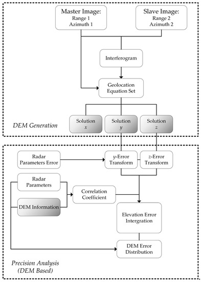
Figure 1.
Flowchart of digital elevation map (DEM) generation and precision analysis method.
2.2. Key Problems in GB-InSAR DEM Generation
GB-InSAR systems have unique characteristics, including their system parameters, observation geometry, and observation objects. The most typical features are the wide beams and viewing span, which are from tens of meters to several kilometers. Since its synthetic aperture length is subject to equipment costs and installation conditions, its azimuth resolution also suffers, and a large number of synthetic apertures are incomplete. The problem in the imaging process is briefly discussed in the next part, while this section mainly discusses the plane-wave approximation error, the invalidation of the flat-phase removal, and baseline approximation error. The latter is caused by the azimuth angle of the target and the baseline angle itself.
A GB-InSAR coordinate system is first built on the basis of the following principles: The x-axis lies in the horizontal plane. Usually, it coincides with the synthetic aperture direction, but the situation involving an angle between the horizontal plane and synthetic aperture direction is also discussed below. When acquiring the master image, the transmitting and receiving antennas move along the master rail simultaneously to generate the synthetic aperture. The y-axis is perpendicular to the x-axis in the horizontal plane, and the z-axis is perpendicular to the xy-plane. Cartesian coordinates can be used to represent a DEM only in this configuration since the z-axis is parallel to the altitude. The baseline is usually located in the yz-plane and starts from the origin point, but the situation in which a random angle exists between the baseline and the master rail direction is also discussed. The baseline length is B, and the angle including the z-axis is α. When acquiring the slave image, the transmitting and receiving antennas move along the slave track, and the center of this synthetic aperture is located at the end of the baseline. Therefore, the geometric relationship of the GB-InSAR system is as depicted in Figure 2.
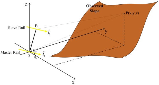
Figure 2.
Ground-based interferometric synthetic aperture radar (GB-InSAR) system coordinates.
In flat-phase removal, the interferometric phase is usually decomposed into a flat phase and an elevation phase in air-/spaceborne InSAR systems. This reduces the density of the phase stripe, and the remaining elevation phase is directly proportional to the target’s height. Expanding on this idea, a flat-phase removal step is used in GB-InSAR. However, a good conclusion cannot be reached since the assumption that the slant range is much bigger than the target’s height is no longer suitable.
Without loss of generality, considering a target P and its corresponding point P′ on a flat plane, the elevation phase can be calculated by subtracting the phase caused by r and r1 from the phase caused by r and . The sketch map is as depicted in Figure 3. Since the slant range R is comparative to the target height h, only when the baseline angle is can represent the target’s height. Equation (1) shows that is not directly linearly dependent on height but coupled with other terms in the ground-based situation. Thus, there is no need to decompose the interferometric phase into the elevation phase,
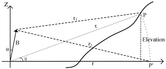
Figure 3.
Flat-phase removal in GB-InSAR.
The plane-wave approximation error and baseline distortion error all originate from the geometric approximation. Specifically, the plane-wave error means that the range of the difference between master and slave images is not determined only by the baseline parallel component ; the baseline distortion error means that the baseline component, especially the baseline angle, is not a constant throughout the whole scene since the plane determined by the baseline vector and target is adaptive to the target position and not always vertical. A simulation is described in this section in order to show the forms of those errors. An ideal slope with a typical range and gradient is chosen, and the error between the ideal slope and the DEM generated by Reference [7] is acquired. The curves along the range (Figure 4a) and azimuth (Figure 4b) are extracted from the surface error. The elevation error curves are depicted as the plane-wave error along the slant range and the distortion error along the azimuth direction. It is clear from Figure 4 that those errors have a significant influence in the situations involving a short slant range area and huge azimuth angle area, which are quite common in ground-based scenarios. The former error may reach the meter level, and it decreases as the range increases; the latter error may reach the level of tens of meters, and it decreases as the azimuth decreases.
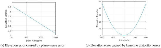
Figure 4.
The key problems in GB-InSAR DEM generation.
In a word, the key challenge in GB-InSAR DEM generation is to achieve good precision in a short slant range and huge azimuth area by not decomposing the interferometric phase component.
2.3. GB-InSAR Geolocation Method
The GB-InSAR system has a wide beam and a scene breadth comparative to the slant range, and it obtains vast sub-aperture. The typical imaging algorithm for GB-InSAR is the back-projection (BP) algorithm in polar coordinates [13]. Considering the BP algorithm through the matched-filtering theory, each signal is matched with the time delay pause, where the delay is determined by the pixel range and azimuth angle. Then, all the matched signals are accumulated together to generate the pixel result. The best match calculated by the time delay in the spatial domain is equivalent to the Doppler information in the Doppler domain described by the range-Doppler (RD) algorithm, which means that the point set with the same time delay is equivalent to a point set with a corresponding Doppler frequency.
where, R is the distance to the original point, is the azimuth angle, and is the antenna’s position from the original point. Thus, the information from an image pair includes two slant ranges, two azimuth angles, and a single interferogram.
where, , represent the master/slave track direction vector, represents the baseline vector, is the signal wavelength, and is the interferometric phase. There are many schemes that can be used as the basis of building the geolocation equation set, such as Scheme 1, with two slant range and an azimuth angle; Scheme 2, with two azimuth angles and a slant range; and Scheme 3, with a slant range azimuth angle and interferogram. In the ground-based interferometry situation, the key problems are the data-acquisition geometry and image coordinate errors.
On the one hand, the sensitivity between the different equations will be influenced by the data-acquisition geometry, including the baseline length and track direction differences. The baseline in the GB-InSAR system is usually tens of centimeters, so equation and equation differ little in their range constraints. This means that Scheme 1 will experience a loss of accuracy because equation is insensitive to the solution set satisfied with equation . Further, the master rail direction is usually parallel to the slave direction in the GB-InSAR system, and the baseline is also perpendicular to the rail direction. So, Scheme 2 will also be invalidated. By extracting equation from equation , the equation turns into , which means that the last equation in Scheme 3 only introduces invalid information, which we can directly acquire from the system configuration, and the right side of the equation will always stay the same since both of them represent the target’s x-coordinate. Actually, the geolocation based on range and azimuth angle always fits the huge baseline and huge master/slave direction difference data acquisition situations instead of interferometry cases.
On the other hand, data errors are usually the result of quantization error by radar 2D resolution. Thus, the error from the range resolution and azimuth resolution is usually at the decimeter level, where W is the signal bandwidth and L is the synthetic aperture length. By using the interferometry technique, the range difference can be corrected to the wavelength level, a centimeter level in Ku-band conditions. By extracting equation from equation , the master image is multiplied by the conjugation of the slave image, and the slant range constraint transforms into a plane constraint perpendicular to the baseline direction vector, which is sensitive to the set satisfied by a slant range constraint. Thus, the DEM can only be calculated with the range, azimuth, and interferometric phase information as a result of ground-based baseline conditions,
The physical meaning of the interferometric measurement can be expressed as follows. Equation in Equation (3) represents a sphere determined by the range, and equation in Equation (3) represents a cone determined by the azimuth angle. Therefore, the target point is located in a circle on the range sphere cut by the azimuth cone. When considering the beam width, the target located in an arc on that circle is cut by a beam dihedral angle. The interferometric phase constraint, , can be expressed as a phase hyperboloid, with no approximation involved. The target will be located at the point of intersection between the above-mentioned arc and this cone. The sketch map of this method is depicted in Figure 5. When the original equation set has been transformed into Equation (4) and is expressed as a constant , the first two equations in Equation (4) represent two planes. One is perpendicular to the rail direction vector, and the other is perpendicular to the baseline direction vector. The intersection between those two planes restrict the solution to a small area that faces error fluctuation. However, the other schemes allow the solution to slide along an arc approximatively, and the stability of the solution becomes much worse. That is the key reason that the interferometric technique can achieve better results compared with the traditional geolocation method, although they all suffer from quantization errors.
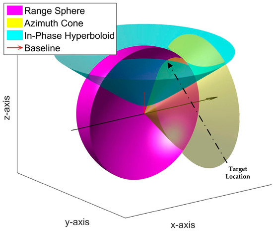
Figure 5.
Geometric relationship of the location equation set.
Usually, the rail error and baseline vertical error are ignored, which means
where is the baseline incident angle. Thus, the analytical solution is acquired. The influence of the baseline angle is shown in the rotation matrix, and the azimuth influence is shown in the last vector,
Considering the most general situation in the GB-InSAR system, the rail direction vector and the baseline direction vector degenerate into the following condition. With respect to the rail direction, the ‘yawing angle’ only influences the system’s illuminated area and has no influence on DEM generation. Thus, only the ‘rolling angle’ is taken into consideration. The rail direction is not always parallel to the x-axis. In the baseline direction, the dip angle in the yz-plane is already modeled as the baseline angle. So, between the baseline direction vector and the rail direction vector, which is no longer 90°, is considered. The most general form of the direction matrix A can be decomposed into three parts, shown in Equation (7), and the form in Equation (5) is a special case when and ,
Since the rotation matrix is an orthogonal matrix and does not influence the slant range’s description, the solution can be acquired on the basis of and multiplied by . This solution can be used to represent the most general situation in the GB-InSAR system. The following section’s analysis still uses the solution in Equation (5), since Equation (8) is much too complex, and the two angles can retain small values,
3. GB-InSAR System Precision Analysis
3.1. Error Transfer in the GB-InSAR System
According to the solution in Equation (6), the obtained parameters include the range R, azimuth angle , baseline length B, baseline inclination , interferometric phase , and wavelength . The error from and are small enough to ignore. Thus, the four main error sources are R, B, , and . It is clear that only exists as a form of the rotation matrix, so in regard to the relative error, the number of error sources decreases to three. Additionally, with regard to the absolute error, such as that which occurs when assessing the DEM precision with another reference, the four error sources remain.
The error from the parameters affects the target coordinates. In the ground-based situation, the elevation measurement is affected not only by the z-coordinate but also the y-coordinate. This effect happens especially in high-steepness areas and has a close relationship with the surface gradient. With the equation solution above, the delivery relationship is analyzed in the y- and z-direction since the x-axis coordinate is only decided by the imaging parameters and is independent of interferometric parameters. The transfer coefficients are shown in Table 1.

Table 1.
Error transfer coefficients.
When the errors themselves are small values, the system’s error can be integrated by the total differential in each direction
The final system error can be approximately united into a single direction (z-direction) by the gradient angle of the scene. is the slope gradient for each pixel of the scene and is defined as the ratio that relates the z-increment to the y-increment. It can be acquired by fitting the local plane according to the DEM produced.
It is worth mentioning that , , , and on the right side of the equation represent the real errors that occur during the DEM generation process, and the error on the left side of the equation refers to the exact DEM error. Usually, during a simulation analysis, we have the errors’ statistical features, such as , , , , instead of the true value of a single implementation. Thus, the system error needs to be integrated using the following rules. The left side of this equation also represents the errors’ statistical features of the DEM instead of the real DEM error
During the experiment, it is hard to achieve a repetitive system’s configurations to complete the statistical analysis, and it is also hard to get the exact error during the experiment. Thus, in order to use Equation (9) or Equation (11), the data processing step is required, and it is discussed in detail in Section 4.
3.2. Coherence Analysis in the GB-InSAR System
The previous section presents the analysis of the error delivery coefficient, and analysis of the error sources themselves are illustrated in this section. Among these error sources, the slant range R, baseline length B, and baseline angle can be modeled with simple distributions. The slant range is subjected to a uniform distribution with a constant offset, , written as . The baseline angle and baseline length, as the measurement error, are subject to Gaussian distributions with zero-means: , .
The interferometric phase , however, is hard to model with a simple distribution since it has many influencing factors. However, References [14,15] analyzed the probability density function of the interferometric phase and revealed the relationship between the correlation coefficient and the standard deviation. Thus, the analysis of the GB-InSAR interferometric phase error becomes the GB-InSAR decorrelation sources.
The correlation coefficient is a typical criterion that is used to evaluate the coherence between two sequences, . In InSAR interferogram processing, the correlation coefficient usually shows the interferogram’s phase noise level, so the lower correlation coefficient is the lower confidence level of the interferogram and will be the same as the higher standard deviation of the interferometric phase. An identical master/slave pair, or in general, a well-generated interferogram with clear phase stripes, can achieve a good correlation coefficient because the phase caused by the terrain is still much smoother and more stationary than the noise. Since it is hard to achieve a sequence for every pixel, a spatial averaging technique is used instead of sequential averaging, which generally means .
3.2.1. GB-InSAR Decorrelation Sources
The decorrelation sources in the InSAR system are generally thermal decoherence, spatial decoherence, and temporal decoherence. The temporal decoherence primarily contains the changes in the atmosphere and surface features. Only the changes in the atmosphere and surface are taken into consideration, rather than the atmosphere and surface themselves. Furthermore, the transmission delay in the ground-based situation can be ignored,
is influenced by the temperature T, humidity e, and air pressure P [16]; thus, is influenced by the change in temperature, humidity, and air pressure, as shown in the formula below. GB-InSAR’s data acquisition time usually stays at the level of minutes. According to the existing atmosphere analysis result [17], the changes in T, e, and P are calculated in terms of hours, so fluctuations in terms of minutes can be ignored,
The deformation has an influence on the correlation coefficient, as indicated in the formula below [18]. The surface has been modeled and its deformation standard deviations in two directions are the main influencing factors. In the equation below, is the incident angle of the surface,
Obviously, the deformation standard deviations depend on the surface category. In vegetated areas, the leaves and grasses have strong reflectance, causing an invalidation of interferometric processing. According to a recent analysis result [19], the deformation standard deviation of a bare slope surface can be less than 1 mm during the minute’s data acquisition. So, GB-InSAR decorrelation sources are mainly thermal decoherence and spatial decoherence.
3.2.2. Theoretical Formula of the GB-InSAR Correlation Coefficient
On the basis of the former chapter, the correlation coefficient can be integrated as , and (signal/noise ratio) represents thermal decoherence. According to the signal model [20],
We have the formula . Since the GB-InSAR system has a scene breadth comparative to the slant range and a variable incident angle, and need to be decomposed to a more accurate level. , where represents a radar system factor [21]. By using the scatter model introduced by Ulaby [22], we can acquire a surface radar cross-sectional formula, . Here, we use vertical-transmitting and vertical-receiving polarization, the Ku-band, and a rocky scene as an example,
The specific form of the parameter is given below, and the components in all represent radar system parameters. In an air-/space-borne situation, thermal decoherence is calculated by a simple signal model, regardless of the factors that influence the target radar cross-section and ,
With regard to spatial decoherence, the observation scenes of GB-InSAR are kinds of slope terrain, and the gradient and slope orientations are changeable. GB-InSAR also has a huge span in its slant range and azimuth angle. Therefore, spatial decoherence must be analyzed in 3D space. The detailed derivation process is given in the Appendix A.
An echo model of the scattering infinitesimal plane unit is built as
Given the independence of between different pixels, we can derive a simplified conjugate product result.
where and are the two-dimensional resolutions along the target infinitesimal plane, and they are generated by the range resolution and azimuth resolution in the SAR system. W is the signal bandwidth, and is the synthetic aperture length. They are influenced by the two incident angles, and ,
The equation in the integral is a Fourier integration, so results in a triangle envelope. Its shift from the peak is caused by the viewing angles. Since the x- and y-directions are orthogonal, the total spectrum energy has a pyramid-like form. To build the relationship between the baseline and the viewing angles, the interferometric expression can be transferred into
Therefore, the viewing angle change caused by the baseline shifts the ground frequency spectrum, and the correlation coefficient is reduced with the overlap spectrum. and are the baseline components, which influence the viewing angle in the two directions,
We finally get the total expression for the GB-InSAR correlation coefficient; below, it is compared with the traditional spaceborne correlation coefficient. In a 3D observation scene, the spatial decoherence includes a side-look spatial item and a squint spatial item,
In this formula, R represents the target slant range, represents the beam incident angle, W represents the system bandwidth, represents component of the incident angle in the vertical plane, represents the target azimuth angle, represents the system synthetic aperture, and and are the components of that contribute to the side-looking spatial decoherence and squint spatial decoherence. R, , , , , and in the formula all change with the target positions in the viewing scenes. Thus, the correlation coefficient in a single scene has a clear spatial distribution.
In an air-/spaceborne situation, the spatial formula is only integrated in the 2D plane because of the long slant range, narrow beam, and fixed azimuth resolution. All these factors lead to small decoherence of the squint spatial form. Thus, thermal decoherence is usually set as a constant, and spatial decoherence only considers side-looking decoherence.
In this experimental scene, there is a large squint slope for which the correlation coefficient is much lower than in the other areas. With the typical formula, the correlation coefficient is still higher than 0.9, which cannot fit the real data results. However, the proposed formula, with the corrected thermal decoherence and a squint spatial decoherence item, matches well with the real data. The details of the correlation coefficient result are shown in Section 4.
3.3. Error Spatial Distribution
Although most of the error sources generally have no connection to the target positions, the positional information, including R, , and , influence the transfer coefficient in Table 1, and this effect leads to a different coordinate error. Moreover, the correlation coefficient changes with the target’s position according to Equation (24), and the interferometric phase itself also changes.
It is also worth mentioning that the spatially related error is influenced by not only the target’s position vector but also the local normal vector and the slope gradient. For this reason, the analysis based on a single or a group point at the typical value cannot accurately represent the system’s performance.
Equation (11) was applied in the simulation to analyze the error’s statistical performance. The InSAR coordinate was built as mentioned in Section 2, and the baseline stayed in the yz-plane. The DEM was a simulated part of the paraboloid since it has a different range, gradient, and orientation. The spatial information was acquired from the 3D information. Then, the correlation coefficient was calculated as in Section 3.2 in order to get the interferometric phase error, and the other error sources were set to m, mm and . The error is shown in Figure 6.
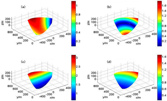
Figure 6.
DEM theoretical error distributions by each error sources: (a) Slant range, (b) baseline length, (c) baseline angle, (d) in-phase.
According to the surface plots, the slant range error mainly influences the front area of the scene. The baseline length error mainly influences the area with a short slant range and huge viewing angle, such as those in the bottom area. A stripe area at the top of the slope is insensitive to the baseline length error. The demand of the baseline length precision will decrease if the observation area is mainly spread in the stripe. The baseline angle error only influences the absolute DEM accuracy by a kind of coordinate rotation; thus, the larger the slant range of the pixels, the higher the error obtained. It is obvious that the decrease in the observation range decreases the demand of the baseline angle precision.
The errors caused by the interferometric phase do not have obvious continuity since the error source itself is mainly spread in an area that is hard to achieve a well correlation coefficient, including the large incident, overlap and shadow areas. For example, this is the case in the right area with a large azimuth angle. According to the theoretical formula, the measurement error caused by the interferometric phase ranges from the level of centimeters to as high as tens of meters. However, an area with a low correlation coefficient will be excluded from the interferometric area, and the phase filtering part of data processing can also reduce the phase error [23]. Thus, the maximum error from the interferometric phase is limited since the estimation value from the extremely low coherence area is meaningless, but the distribution for the entire scene may appear similar.
It is worth mentioning that there are great differences between each error in the same scene, and they are not obviously relevant to the slant range or azimuth angle. This is because the DEM information comprises not only the range and azimuth information but also the incident angle, surface gradient, and slope orientation. The described method is important when optimizing the use of a GB-SAR interferometer or, in other words, when selecting the appropriate baseline for different viewing scenes.
4. Results
4.1. GB-InSAR System and LiDAR Data Acquisition
The GB-InSAR system employed in this study is designed and manufactured by the Beijing Institute of Technology. The radar instrument and the observation scene are shown in Figure 7. The radar system includes Ku-band frequency-modulation continuous-wave radar, a horizontal rail to generate synthetic aperture, an outside holder to achieve the spatial baseline, and a personal computer for operational control and data processing. The experiment field chosen was an open-pit in Hebei, China. The area is a high-steepness rocky slope with three main different slope orientations (the bottom, the front, and the right). The slant range is from 200 m to 900 m, and the azimuth angle range is from −30° to 30°.
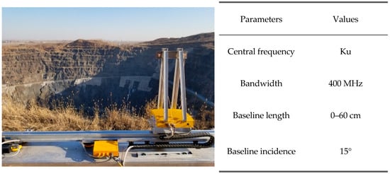
Figure 7.
Sketch map of the GB-InSAR system and the experiment field.
Since the radar transmits a continuous wave, the transmitting antenna and receiving antenna work simultaneously. The GB-InSAR works in the repeat-pass mode. By moving both antennas along the rail, the synthetic aperture is achieved, and by shifting both antennas along the holder, the equivalent phase center is shifted, and the spatial baseline is achieved [24].
In addition to the radar system, the experiment also used a high-precision LiDAR system (LMS-Z620) to acquire the DEM product in order to compare it with the DEM generated by GB-InSAR. The system’s configuration with the radar and LiDAR original data are shown in Figure 8. This result can be used in the subsequent correlation coefficient verification and DEM error distribution analysis.
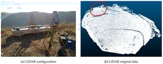
Figure 8.
Light detection and ranging (LiDAR) configuration and its original data.
From Figure 8, the LiDAR and radar are situated so that they are as close as possible without covering each other. LiDAR cannot realize a horizontal observation. The point cloud of LiDAR is dense enough that down-sampling is performed to get a DEM with a 3 × 3 m resolution in order to better match the radar data. Since the DEMs generated by radar and LiDAR are in different coordinates, three corner reflectors were situated on the left side of the top of the slope for the transformation between those two coordinates. Radar can recognize ground control points (GCPs) by the image amplitude, but LiDAR must use local depth sampling (the red circled area in Figure 8) to obtain the structure of the corner reflector. Finally, the reformatted and coordinate-calibrated LiDAR DEM is acquired.
4.2. Verification of the Correlation Coefficient Calculation
This part aims to demonstrate the verification of the correlation coefficient calculation. There are two ways to calculate the correlation coefficient: From real SAR images and from system parameters and object parameters. The result of Equation (24) should match the result of the image. Since this part only verifies the correctness of the formula, the DEM is already known.
The GB-InSAR system, on one hand, has a low azimuth resolution; on the other hand, the system generally monitors the high-steepness slope area. In the “long” baseline condition, the interferometric phase stripe can be so dense that the phase differences caused by the terrain in a single estimation window may reach a level. In order to get the correct correlation coefficient from the GB-InSAR real data, Equation (25) with slope compensation is used [25]. Here, we already have the existing DEM data provided for the model correlation coefficient, Equation (24) and the real coefficient, Equation (25). In the below equation, N is the total number of pixels in the estimation window, and and are the corresponding pixels’ complex values in the master and slave window,
Choosing both 15 cm and 45 cm interferometric pairs, the real data correlation coefficient is calculated by the formula above. The result is matched with the SAR image of the scene depicted in the first picture of each group in Figure 9. The theoretical result, the thermal decoherence part, and the spatial decoherence part are depicted in the other three pictures.
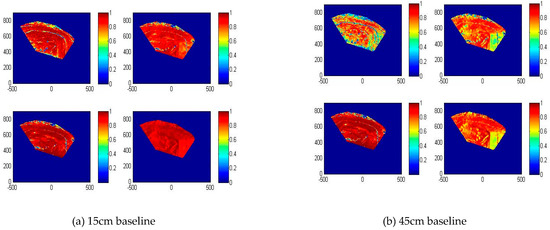
Figure 9.
Two groups of correlation coefficient distributions. Real-data result (upper left), theoretical result (upper right), thermal decoherence part (lower left), and spatial decoherence part (lower right).
The result shows that in short baseline conditions (15 cm), the main factor of the correlation coefficient is the thermal decoherence part; in long baseline conditions (45 cm), the thermal decoherence part basically remains unchanged, while the spatial decoherence becomes the main factor. Both decoherence sources have obvious spatial distributions. The former is strongly influenced by incident angles, and the main factor is reflected by the lane in the middle and the flat area at the top. The latter is strongly influenced by the squint part item, . Even in the 45 cm baseline condition, the front part and bottom part of the pit can still acquire a correlation coefficient of 0.7, but the coefficient of the right part decreases to 0.5.
Figure 10 compares the coefficient statistical distribution calculated by different formulas using the 45 cm conditions in Figure 9. It is clear that the curve calculated by the original Equation (24) (green line) widely deviates from the real-data curve (blue line) generated by Equation (25), but the curve calculated by Equation (24) (red line) is similar to the real-data curve.
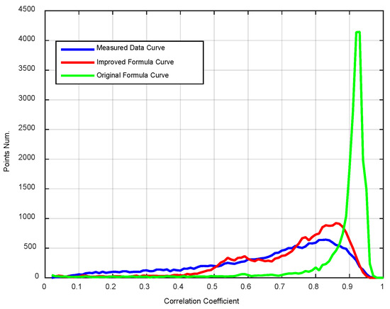
Figure 10.
Comparison of the correlation coefficient distribution obtained by different methods.
4.3. DEM Precision and Error Distribution
In this section, the DEM generated by GB-InSAR is compared with the DEM generated by the high-precision LiDAR. Both DEMs were registered by using the corner reflectors as the ground control points. The results for the 3D surface model are shown in Figure 11.
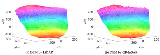
Figure 11.
DEM by LiDAR and GB-InSAR.
First, the data processing methods are succinctly summarized in this part. The first step is interferogram generation. After that, a two-step phase filtering method is used to reduce the speckle noise. A Goldstein filter is used to preprocess the low-coherence area, and a global gradient-adaptive filter is used to lower the noise and maintain the stripe edges at the same time. The unwrapping method is based on minimum flow cost, and a ground-control-point (GCP) is used to get the absolute unwrapped phase. Finally, the DEM is generated by the equation in Section 2.
According to the results, the LiDAR DEM is set as the true value, and the GB-InSAR DEM is estimated. The DEM error is acquired by subtracting these two DEMs, and both the statistical and spatial distributions of the error can be determined. The statistical distribution of the error is shown in Figure 12. A Gaussian distribution is used to fit the real-data histogram, and the mean value and standard deviation of the fitting curve are 0.2 m and 2.9 m, respectively. These values prove the effectiveness of the DEM generation formula proposed in this paper.
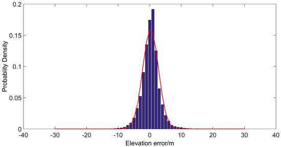
Figure 12.
Statistical distribution of the DEM error and a Gaussian fitted curve.
The error spatial distribution in the whole observation scene is shown in Figure 13. In the experiment, the system parameters, such as the baseline angle and baseline inclination, achieved good precision. The main error sources are the slant range and interferometric phase. The theoretical error is acquired by the method proposed in Section 3, for example, the transfer coefficient in Table 1 and integration Equations (9) and (10). The DEM used in the precision analysis is shown in Figure 14, and the correlation coefficient is depicted above in Figure 9. The theoretical error is mainly located at the top of the pit, the median lane, and the bottom gully. The real-data error does not have good continuity, but the error at the top is still larger than at the bottom. The top and the bottom gully can fit the theoretical error.
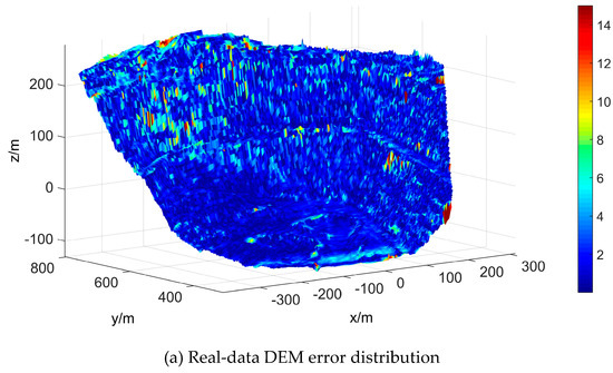
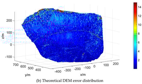
Figure 13.
Real-data and theoretical spatial distribution of the DEM error.
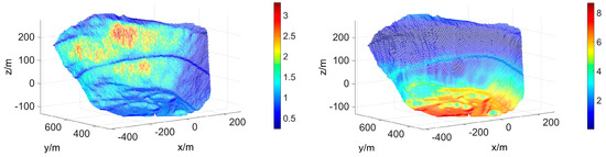
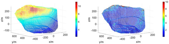
Figure 14.
DEM theoretical error distributions by each error source: Slant range (upper left), baseline length (upper right), baseline angle (lower left), in-phase (lower right).
In fact, the data error is acquired by comparing the InSAR–DEM to the LiDAR–DEM. The error introduced by data processing and data registration also influence the final error, but the theoretical error only considers the system part. Thus, the theoretical error can fit the real data well when the system error is the main error source, and performance is poor if the main errors are due to data processing and mismatch. Moreover, as is mentioned in Section 3.3, the phase error caused by a weak correlation coefficient can be compensated by phase filtering; therefore, a low-correlation area can still get good results, which makes the theoretical error stronger than the real data. This scenario is the case for some parts of the lane.
The former result shows a general effect of the GB-InSAR system and its DEM precision. It is also important to analyze the error distribution with different main error sources. Thus, Figure 14 shows the theoretical distributions of different error sources in the test field, and Figure 15 shows the error distribution when the main error sources become the baseline length or baseline inclination. Table 2 shows a comparison between real and theoretical errors for the different error sources.
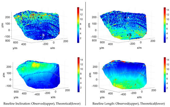
Figure 15.
DEM error distributions with different main error source situations.
Table 2.
Comparison between real-data error and theoretical error in different situations.
For the baseline inclination, the error is set to 0.5°. The area with a larger slant range has a larger DEM error. For the baseline length, the value in the experiment is 15 cm. In the DEM generation step, a 10 mm baseline length error is added, so the DEM is generated by the baseline parameters at 16 cm. It is clear that the bottom part is more influenced than the top stripe area. The theoretical error distribution for each situation has the same tendency compared with its main error sources shown in Figure 14. Two test sets, denoted A and B, were chosen from the front slope and the bottom slope. The average error differences between theory and reality are smaller than 1 m, showing that the precision analysis method can fit the real data better if the main error sources are from the system parameters, as shown in Table 2.
5. Conclusions
A GB-InSAR system has unique features for observation geometry and observation objects. On one hand, these features lead to the invalidation of the elevation calculation formula, which is widely used in air-/spaceborne InSAR systems. On the other hand, both decoherence sources and the error transfer coefficient have obvious spatial distributions. The typical point error cannot represent the system performance in whole scenes.
This paper first proposed a 3D coordinate generation formula that was based on the geolocation concept. Then, the error sources were analyzed and modeled using the formula. The calculation method for the correlation coefficient was discussed in detail. Finally, by considering the spatial information of the viewing scene, the error distribution forms of the different error sources were depicted, and a system error distribution diagram at a meter-level resolution was provided.
The experiment resulted in two DEMs, one from the GB-InSAR system and one from the LiDAR system. By comparing the two DEMs, the statistical distribution of the error was first acquired with a mean value of 0.2 m and a standard deviation of 2.9 m. Second, the application of the correlation coefficient calculation method matched the real-data much better than the typical method. Finally, the error spatial distributions from theory and real data were compared. Since the error of the real data included not only the system error but also the data processing error and the mismatching error, the results from the theory and real data were not exactly the same. However, they still fall within a reasonable bound. When increasing system errors, such as the baseline length error or the baseline inclination error, the result of theory compared with that of reality is satisfactory.
Author Contributions
Conceptualization, W.T. and Z.Z.; methodology, Z.Z.; validation, W.T. and Z.Z.; formal analysis, Z.Z.; writing—original draft preparation, Z.Z.; writing—review and editing, J.W.; supervision, W.T. and C.H.; funding acquisition, T.Z. and C.H.
Funding
This work was funded by the National Natural Science Foundation of China (Grant Nos. 31727901, 61601031, 61427802, 61625103), the Chang Jiang Scholars Program (Grant No. T2012122), and the 111 Project of China (Grant No. B14010).
Conflicts of Interest
The authors declare no conflict of interest.
Appendix A
As mentioned in Section 3.2, spatial decoherence must be analyzed in 3D space, so the echo model needs to be established based on a 3D surface. An echo model of the scattering infinitesimal plane unit is built as
where represents the complex backscatter, r represents the range of the slant relative to the center of the target infinitesimal plane, and are the coordinates in the infinitesimal plane that describe the position relative to the center of the plane. is the system impulse response and is a two-dimensional “sinc” function. is the integration of all scatter points in this infinitesimal plane, as well as the echo of this infinitesimal plane.
The variable is defined in the vertical plane spanned by the z-axis unit vector and the target’s position vector. The target’s infinitesimal plane has a normal vector and a normal vector component in the above vertical plane. Thus, is the included angle between the target’s position vector and normal vector component, and it represents the beam’s incident angle in this vertical plane,
where is the infinitesimal plane’s normal vector, , and . Similarly, is defined in the plane spanned by the target’s position vector and the target’s horizontal vector . The target infinitesimal plane normal vector also has a component in the plane above. Thus, is the included angle between the target position vector and normal vector component, and it represents the beam’s incident angle in this plane. The sketch map of the geometry relationship between and are shown in Figure A1

Figure A1.
Sketch map of the geometry relationship about (left) and (right).
Therefore, for the point in the infinitesimal plane, if the target offset to the center is , the slant range can be calculated by . Thus, we have the same form of this infinitesimal plane in the slave image,
The interferometric processing method can be described as a four-integral expression:
The different scattering targets in an infinitesimal plane are independent of others, and interference only occurs for a perfect match [26], . Thus, we have a simplified conjugate product result,
where and are the two-dimensional resolutions along the target infinitesimal plane, and they are generated by the SAR system’s range resolution and the azimuth resolution. W is the signal bandwidth, and is the synthetic aperture length. They are influenced by the two incident angles and ,
The equation for the integral is a Fourier integration, so results in a triangle envelope. Its shift from the peak is caused by the viewing angles. Since the x- and y-directions are orthogonal, the total spectrum energy in 3D space has a pyramid-like form. To build the relationship between the baseline and the viewing angles, the interferometric expression can be transformed into
Therefore, the viewing angle change caused by the baseline shifts the ground frequency spectrum, and the correlation coefficient reduces with the overlap spectrum. and are the baseline components, which influence the viewing angle in the two directions
References
- Pieraccini, M.; Luzi, G.; Atzeni, C. Terrain mapping by ground-based interferometric radar. IEEE Trans. Geosci. Sens. 2001, 39, 2176–2181. [Google Scholar] [CrossRef]
- Casagli, N.; Farina, P.; Leva, D.; Nico, G.; Tarchi, D. Landslide monitoring on a short and long time scale by using ground-based SAR interferometry. In Proceedings of the International Symposium on Remote Sensing, Baltimore, MD, USA, 6–11 October 2003; Volume 4886, pp. 322–329. [Google Scholar]
- Fuster, R.M.; Usón, M.F.; Ibars, A.B. Interferometric orbit determination for geostationary satellites. Sci. China Inf. Sci. 2017, 60, 060302. [Google Scholar] [CrossRef]
- Lanari, R.; Fornaro, G.; Riccio, D.; Migliaccio, M.; Papathanassiou, K.P.; Moreira, J.R.; Dutra, L.; Puglisi, G.; Franceschetti, G.; Coltelli, M. Genreation of digital elevation models by using SIR-C/X-SAR multi-frequency two-pass interferometry: The Etan case study. IEEE Trans. Geosci. Remote Sens. 1996, 34, 1097–1112. [Google Scholar] [CrossRef]
- Pieraccini, M.; Casagli, N.; Luzi, G.; Tarchi, D.; Mecatti, D.; Noferini, L.; Atzeni, C. Landslide monitoring by ground-based radar interferometry: A field test in Valdarno (Italy). Int. J. Remote Sens. 2002, 24, 1385–1391. [Google Scholar] [CrossRef]
- Hensley, S.; Rosen, P.; Joughin, I.; Li, F.; Madsen, S.; Goldstein, R.; Rodriguez, E. Synthetic aperture radar interferometry. Proc. IEEE 2000, 88, 333–382. [Google Scholar]
- Noferini, L.; Pieraccini, M.; Mecatti, D.; Macaluso, G.; Luzi, G.; Atzeni, C. DEM by Ground-Based SAR Interferometry. IEEE Geosci. Sens. Lett. 2007, 4, 659–663. [Google Scholar] [CrossRef]
- Martinez-Vazquez, A.; Fortuny-Guasch, J. Averaging and Formulation Impact on GB-SAR Topographic Mapping. IEEE Geosci. Sens. Lett. 2008, 5, 635–639. [Google Scholar] [CrossRef]
- Nico, G.; Leva, D.; Antonello, G.; Tarchi, D. Ground-based SAR interferometry for terrain mapping: Theory and sensitivity analysis. IEEE Trans. Geosci. Sens. 2004, 42, 1344–1350. [Google Scholar] [CrossRef]
- Nico, G. Exact closed-form geolocation for SAR interferometry. IEEE Trans. Geosci. Sens. 2002, 40, 220–222. [Google Scholar] [CrossRef]
- Sansosti, E. A simple and exact solution for the interferometric and stereo SAR geolocation problem. IEEE Trans. Geosci. Sens. 2004, 42, 1625–1634. [Google Scholar] [CrossRef]
- Li, F.; Goldstein, R.M. Studies of multi-baseline spaceborne interferometric synthetic aperture radars. IEEE Trans. Geosci. Remote Sens. 1990, 28, 88–97. [Google Scholar] [CrossRef]
- Meta, A.; Hoogeboom, P. Development of signal processing algorithms for high resolution airborne millimeter wave FMCW SAR. In Proceedings of the IEEE International Radar Conference, Arlington, VA, USA, 9–12 May 2005; pp. 326–331. [Google Scholar]
- Just, D.; Bamler, R. Phase statistics of interferograms with applications to synthetic aperture radar. Appl. Opt. 1994, 33, 4361. [Google Scholar] [CrossRef] [PubMed]
- Lee, J.S.; Hoppel, K.W.; Mango, S.A.; Miller, A.R. Intensity and Phase Statistics of Multi-look Polarimetric and Interferometric SAR Imagery. IEEE Trans. Geosci. Remote Sens. 1994, 32, 1017–1028. [Google Scholar]
- Pieraccini, M.; Mecatti, D.; Noferini, L.; Moia, F.; Atzeni, C.; Luzi, G.; Guidi, G. Ground-based radar interferometry for landslides monitoring: Atmospheric and instrumental decorrelation sources on experimental data. IEEE Trans. Geosci. Sens. 2004, 42, 2454–2466. [Google Scholar]
- Iglesias, R.; Fabregas, X.; Aguasca, A.; Mallorqui, J.J.; Lopez-Martinez, C.; Gili, J.A.; Corominas, J. Atmospheric Phase Screen Compensation in Ground-Based SAR with a Multiple-Regression Model Over Mountainous Regions. IEEE Trans. Geosci. Sens. 2014, 52, 2436–2449. [Google Scholar] [CrossRef]
- Gabriel, A.K.; Goldstein, R.M.; Zebker, H.A. Mapping small elevation changes over large areas: Differential radar interferometry. J. Geophys. Res. Biogeosci. 1989, 94, 9183. [Google Scholar] [CrossRef]
- Hu, C.; Zhu, M.; Zeng, T.; Tian, W.; Mao, C. High-precision deformation monitoring algorithm for GBSAR system: Rail determination phase error compensation. Sci. China Inf. Sci. 2016, 59, 082307. [Google Scholar] [CrossRef]
- Barber, B.C. The non-isotropic two-dimensional random walk. Waves Random Media 1993, 3, 243–256. [Google Scholar] [CrossRef]
- Long, M.W. Radar Reflectivity of Land and Sea; Artech House: Norwood, MA, USA, 1983. [Google Scholar]
- Ulaby, F.T. Microwave Remote Sensing, Vol: Microwave Remote Sensing, Fundamentals and Radiometry; Addison-Wesley Publishing Company: Boston, MA, USA, 1981. [Google Scholar]
- Goldstein, R.M.; Werner, C.L. Radar interferogram filtering for geophysical applications. Geophys. Res. Lett. Mar. 1998, 25, 4035–4038. [Google Scholar] [CrossRef]
- Bräutigam, B.; Bachmann, M.; Schulze, D.; Tridon, D.B.; Rizzoli, P.; Martone, M.; Gonzalez, C.; Zink, M.; Krieger, G. TanDEM-X Global DEM Quality Status and Acquisition Completion. In Proceedings of the 2014 IEEE Geoscience and Remote Sensing Symposium, Quebec City, QC, Canada, 13–18 July 2014; pp. 3390–3393. [Google Scholar]
- Mandel, L.; Wolf, E. Optical Coherence and Quantum Optics; Cambridge University Press: Cambridge, UK, 1995. [Google Scholar]
- Zebker, H.; Villasenor, J. Decorrelation in interferometric radar echoes. IEEE Trans. Geosci. Sens. 1992, 30, 950–959. [Google Scholar] [CrossRef]
© 2019 by the authors. Licensee MDPI, Basel, Switzerland. This article is an open access article distributed under the terms and conditions of the Creative Commons Attribution (CC BY) license (http://creativecommons.org/licenses/by/4.0/).