Abstract
We have developed a method for evaluating the fidelity of the Aerosol Robotic Network (AERONET) retrieval algorithms by mimicking atmospheric extinction and radiance measurements in a laboratory experiment. This enables radiometric retrievals that use the same sampling volumes, relative humidities, and particle size ranges as observed by other in situ instrumentation in the experiment. We use three Cavity Attenuated Phase Shift (CAPS) monitors for extinction and University of Maryland Baltimore County’s (UMBC) three-wavelength Polarized Imaging Nephelometer (PI-Neph) for angular scattering measurements. We subsample the PI-Neph radiance measurements to angles that correspond to AERONET almucantar scans, with simulated solar zenith angles ranging from 50 to 77. These measurements are then used as input to the Generalized Retrieval of Aerosol and Surface Properties (GRASP) algorithm, which retrieves size distributions, complex refractive indices, single-scatter albedos, and bistatic LiDAR ratios for the in situ samples. We obtained retrievals with residuals less than 8% for about 90 samples. Samples were alternately dried or humidified, and size distributions were limited to diameters of less than 1.0 or 2.5 m by using a cyclone. The single-scatter albedo at 532 nm for these samples ranged from 0.59 to 1.00 when computed with CAPS extinction and Particle Soot Absorption Photometer (PSAP) absorption measurements. The GRASP retrieval provided single-scatter albedos that are highly correlated with the in situ single-scatter albedos, and the correlation coefficients ranged from 0.916 to 0.976, depending upon the simulated solar zenith angle. The GRASP single-scatter albedos exhibited an average absolute bias of +0.023–0.026 with respect to the extinction and absorption measurements for the entire dataset. We also compared the GRASP size distributions to aerodynamic particle size measurements, using densities and aerodynamic shape factors that produce extinctions consistent with our CAPS measurements. The GRASP effective radii are highly correlated (R = 0.80) and biased under the corrected aerodynamic effective radii by 1.3% (for a simulated solar zenith angle of ); the effective variance indicated a correlation of R = 0.51 and a relative bias of 280%. Finally, our apparatus was not capable of measuring backscatter LiDAR ratios, so we measured bistatic LiDAR ratios at a scattering angle of 173 degrees. The GRASP bistatic LiDAR ratios had correlations of 0.71 to 0.86 (depending upon simulated ) with respect to in situ measurements, positive relative biases of 2–10%, and average absolute biases of 1.8–7.9 sr.
1. Introduction
Aerosol remote sensing is an important tool for understanding the effect of aerosols on the Earth’s climate. Passive remote sensing of aerosols from satellite platforms involves measurement of the scattering field at one or more wavelengths, and then “inferring” the microphysical and optical properties of the aerosols that created the scattering field. The aerosol parameters that can be inferred from scattering measurements—and their robustness—partly depends upon the geometry of the measurements. For instance, the Moderate Resolution Imaging Spectrometer (MODIS) uses a continuously rotating scan mirror for its multi-wavelength measurements, which corresponds to a single scattering angle for each area of ground coverage. The MODIS teams use this information to retrieve aerosol optical depth (AOD), Angstrom exponent, and fine mode fraction [1,2,3,4]. However, the MODIS measurement geometry does not provide enough information to retrieve aerosol absorption or aerosol layer height without additional a priori information.
Other satellite instruments—such as the Multi-angle Imaging SpectroRadiometer (MISR) and the Polarization and Directionality of the Earth’s Reflectances (POLDER) —are designed to provide multi-angle measurements at multiple wavelengths foreach location [5,6]. These geometries provide aerosol scattering at 9–12 angles, which increases the information content of the retrievals over single-angle geometries. As a result, additional aerosol parameters can be retrieved from the measurements provided by these instruments, including information about particle non-sphericity and absorption [7,8,9,10].
Perhaps the most reliable aerosol retrievals to date come from the surface-based Aerosol Robotic Network (AERONET), which is a collection of 600+ sun photometers that also have sky-scanning capabilities and are located worldwide [11,12,13,14]. These upward-pointing instruments have narrow fields of view that measure sky radiances at up to 28 scattering angles; AERONET’s upward-pointing geometry is advantageous over satellite viewing geometries because the measurements are uncomplicated by direct surface reflectance. These instruments have another significant advantage over satellite instruments, though—they directly observe the sun’s extinction after it has been attenuated through the atmosphere. Thus, the AERONET instruments measure AOD by application of the extinction law (e.g., [15], Equation (2.23)) instead of inferring it from the scattering field, and this offers a tremendous advantage over downward-pointing satellite viewing geometries for determining aerosol absorption. Routine AERONET products include AOD, aerosol absorption optical depth (AAOD), single-scatter albedo (SSA), complex refractive index, size distribution, asymmetry parameter and phase function (data is available at aeronet.gsfc.nasa.gov). The relative robustness of the AERONET retrievals (compared to satellite retrievals) as well as the uniformity of data processing at hundreds of locations with decades of measurements have rendered AERONET as the de facto standard for validation of satellite instruments and global aerosol models.
Unfortunately, the spatial representation of any AERONET site is much smaller than a global model grid (a global model grid is approximately km at the equator). For instance, the backbone of the AERONET absorption and size distribution retrievals are the almucantar radiance scans (a measurement sequence that scans the sky at a constant viewing zenith angle that is equal to the solar zenith angle). Thus, if all aerosols are located within 5 km of the surface and the solar zenith angle is , then the spatial representation of an almucantar scan is at best 43 km. (That is, the AERONET almucantars outline an inverted right circular cone with an apex angle that is equal to twice the solar zenith angle, or , and the height of the cone is determined by the top height of the aerosol layer. Thus, the maximum horizontal coverage is twice the base radius of the cone; so, for a 5 km aerosol top height this is 5 km). Almucantar scans obtained when aerosols are confined to a 1-km boundary layer and only represent a 2.4 km diameter circle. Thus, a single AERONET site generally represents a small portion of a global model grid. The AERONET team has addressed this issue by regularly establishing sub-grid networks of instruments during NASA field campaigns [16,17], but no field campaign can provide global coverage. Satellite instruments have smaller footprints than models (about 500 m for MODIS, 1.1 km for MISR, and 7 km for POLDER/Parasol at nadir) and their viewing geometries allow for global coverage over a period of days. Consequently, satellite comparisons to AERONET are subject to less sub-grid inhomogeneity than global model comparisons to AERONET. Thus, from a sampling perspective, we should validate satellite retrievals with AERONET (or other surface/airborne measurements) and then validate global models with the satellite retrievals. However, first, we need to evaluate the robustness of the AERONET sky-scan retrieval products.
Validation of the AERONET sky-scan retrievals with in situ measurements remains problematic, even though it has been nearly two decades since the technique was first published [12,13]. Column retrievals such as AERONET are generally difficult to validate with in situ measurements because of several sampling mismatch issues. Traditionally, AERONET validation exercises involve heavily instrumented aircraft flying over an appropriate ground site at a variety of altitudes; the flight data is averaged over the altitude range of the aircraft and compared to the column retrievals. However, it is difficult to obtain many quality comparisons with this approach. Research flight hours are expensive, so flight missions tend to have multiple agendas that may not prioritize spirals over AERONET sites at the low sun elevations required for quality AERONET retrievals (i.e., solar zenith angles greater than 50 degrees). Of course, long flight legs in clear skies may be used instead of spiral descents, but that inevitably results in much larger horizontal sample sizes for the aircraft instrumentation than is observed by the AERONET radiometer (thus adding noise to the comparison). Additionally, sufficient aerosol signal and clear skies over the surface radiometer are required to obtain quality retrievals (AERONET requires at the 0.44 m wavelength for the quality-controlled Level 2 retrievals of aerosol absorption); this happens infrequently during many flight missions, and it is not unusual to end up with only 2–3 flight profiles that correspond to Level 2.0 AERONET sky-scan retrievals for a six week field mission. Flight payloads that fly regularly over AERONET ground sites year-round do not necessarily show better results. For instance, NOAA was only able to obtain one Level 2.0 AERONET SSA for comparison to their Airborne Aerosol Observatory (AAO) profiles after hundreds of flights over the Bondville, Illinois, AERONET site (presented by J. Ogren at the 8th Aerocom workshop in 2009) and the Southern Great Plains (SGP) Cart_Site [18]. Granted, these statistics are somewhat poor because these flights have other agendas and did not necessarily “target” the right conditions for quality retrievals, but the results further illustrate the non-trivial (and expensive) nature of validating column aerosol retrievals with flight data.
Field validation is likely to be even more problematic for the next generation of satellite instruments that are expected to provide aerosol absorption. While there is potential for 10 or more retrievals per day at many AERONET ground sites, scanning radiometers on satellites in sun-synchronized orbits offer one validation opportunity per day at any given location (weather permitting). Opportunities for validation are even worse for so-called “push-broom” imagers such as MISR and LiDARs such as CALIPSO that have narrow fields of view and repeat cycles of approximately 16 days for most locations [5,19,20]. The validation sampling problem for these narrow field of view satellite instruments cannot be solved with large networks of surface radiometers or LiDARs, either. For instance, we compiled statistics for 1.6 years of CALIPSO overpasses within 40 km and 30 min of Level 2.0 AERONET almucantar retrievals (at ∼170 AERONET sites), and found only 40 coincident retrievals; this amounts to an average of 25 coincident retrievals per year. AERONET requires approximately one year of lag time after data acquisition to achieve Level 2.0 status (because of post-field calibration), so it would take approximately 5 years to obtain 100 satellite/AERONET retrieval comparisons. That is too much time for too few comparisons, even if AERONET were robustly validated.
Nonetheless, the AERONET retrieval products have been used extensively as validation tools for global and transport models [21,22,23,24,25,26], computation of the direct radiative effect at various AERONET sites [27], as a possible surrogate for surface concentrations [28,29], and the development of aerosol climatologies [30]. The climatological size distributions and refractive indices derived from the AERONET retrievals have been incorporated into both satellite retrievals and aerosol transport models, and have been used to classify plumes by aerosols type (e.g., [31,32,33]). Additionally, the mismatch between modeled and AERONET column absorption is so significant (factor of 2–4) that some studies have resorted to scaling modeled emissions or AAOD to match the AERONET retrievals worldwide [34,35].
The purpose of this article is to circumvent the remote sensing validation issues described above by assessing the skill of the core AERONET retrieval algorithm, rather than actual retrievals. That is, we apply the column aerosol retrieval algorithm to an in situ sampling volume (instead of using in situ instruments to sample the entire atmospheric column). The advantage of this approach is that the retrieval algorithm is applied to essentially the same aerosol sample as the in situ measurements. We first describe the laboratory apparatus that we use to simulate the AERONET radiance scans, while simultaneously measuring the aerosol optical properties of real aerosols using conventional in situ techniques (Section 3.1). The experiment took place at NASA Langley for a period of four months and resulted in 232 independent aerosol measurements. We call this experiment STEAR, for the Statistical Evaluation of Aerosol Retrievals.
We then describe the GRASP (Generalized Retrieval of Aerosol and Surface Properties) radiometric retrieval algorithm (Section 3.2), which is an evolution of the AERONET algorithm [36,37]. GRASP is a flexible inversion algorithm that admits input from a wide variety of instrument viewing geometries and has already been applied to a wide range of sensors, including POLDER/ADEOS, POLDER/PARASOL, MERIS/Envisat (e.g., [38,39,40,41,42,43]), ground-based AERONET photometers and LiDARs [44], sky cameras [41], polar-nephelometer data [45], and surface measurements of AOD [46]. In addition, GRASP has already been prepared to evaluate Sentinel-4 and 3MI/Metop data and adapted for producing many user-oriented products such as direct radiative forcing [47].
Finally, we recognize that this laboratory approach has limitations as well, and we discuss some of them in Section 5.3 (first and foremost, we do not actually use AERONET instruments for this experiment). Nonetheless, the approach described here provides a valuable “necessary but not sufficient” component of an algorithm assessment process, and should be included in NASA’s program as a supplement to conventional validation techniques. Our experiment and the subsequent discussion focuses on the AERONET retrievals, but this technique can be easily applied to other retrieval algorithms.
2. Rationale
New aerosol retrieval algorithms are typically tested with computational sensitivity studies, but such studies require forward modeling of the scattered radiation field produced by an aerosol-molecular system. Unfortunately, fast forward models can only accommodate aerosol populations with simple shapes that are uniform in composition (i.e., spheres and spheroids that each have a uniform refractive index), whereas real atmospheric aerosols have complicated shapes and compositions. The challenge of complicated shapes can be met to some extent with exact methods such as the discrete dipole approximation (DDA; [48]), but this method suffers from relatively slow computational speeds. Consequently, the DDA method is usually applied to theoretical populations of irregular particles that have only a handful of unique shapes and complex refractive indices (i.e., less than about 10 shapes or refractive indices; [49,50,51,52,53]). Hence, the only way to determine the scattered radiation field produced by a large range of real aerosol populations is to measure the angular dependence of scattering of real particles. The next section describes how we measured the angular dependence of scattering for 232 aerosol populations and used these measurements to evaluate the GRASP algorithm.
3. Method
Although this work emphasizes evaluation of the AERONET retrieval algorithm, we are not actually using the AERONET product (or data from any of the AERONET radiometers, for that matter). Rather, we are working with a newer version of the algorithm called the GRASP [36,37]. The GRASP retrieval algorithm builds upon the legacy code that was first developed for the AERONET surface sun photometers. The algorithm uses kernels that are an expansion of the AERONET kernels, but the input module has enhanced flexibility so that the GRASP algorithm can be applied to a wide variety of airborne, satellite, and surface-based instruments. The GRASP algorithm version 0.7.4 is publicly available at www.grasp-open.com at the time of this writing.
3.1. Experimental Apparatus
Figure 1 shows a schematic of the STEAR laboratory experiment that we created to test the integrity of the AERONET retrieval method. The Polarized Imaging Nephelometer (PI-Neph) provides the angular dependence of scattering that is normally obtained with an AERONET almucantar scan, and the Cavity Attenuated Phase Shift (CAPS) Monitor provides the extinction that is normally obtained with AERONET’s direct sun measurements. Thus, these two instruments act as surrogates for the surface radiometers normally used by the AERONET radiometric inversion code (the appropriateness of this substitution is discussed in Section 5.3). The radiances and extinctions provided by these instruments are used as input to the GRASP retrieval algorithm, and the GRASP algorithm infers the aerosol size distribution and complex refractive index. The aerosol size and refractive index are then used to compute the SSA, extinction-to-backscatter ratio (lidar ratio), asymmetry parameter, and the phase function at all scattering angles. The SSAs provided by GRASP are verified with multiple independent measurements of aerosol absorption (), extinction (), and scattering (). The size distributions provided by GRASP are verified with aerodynamic particle size measurements.
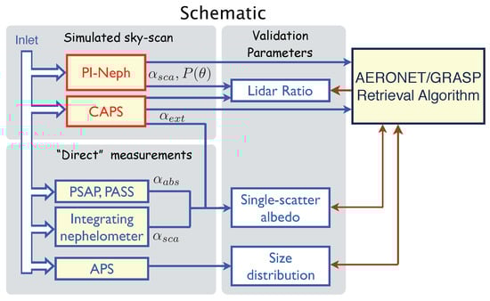
Figure 1.
Apparatus for comparing aerosol remote sensing retrievals to in situ measurements. The Polarized Imaging Nephelometer (PI-Neph) and Cavity Attenuated Phase Shift monitor (CAPS) provide angular scattering and extinction measurements required for the Generalized Retrieval of Aerosol and Surface Properties (GRASP) retrieval algorithm. The GRASP algorithm reports the LiDAR ratio, single-scatter albedo, and the aerosol size distribution; results are verified with “direct” in situ measurements shown in the lower left corner, including the Particle Soot Absorption Photometer (PSAP), the Photo-Acoustic Soot Spectrometer (PASS), an integrating nephelometer, and Aerodynamic Particle Sizer (APS).
The CAPS Monitor is manufactured by Aerodyne Research Inc. It uses very highly reflective mirrors in a cavity that is less than 30 cm in length to obtain very long optical paths (up to 2 km) [54,55]. We incorporated three CAPS instruments in our experiment to obtain particle extinctions at three wavelengths (0.450, 0.530, and 0.630 m). The CAPS instruments have a 1-s response time and a detection level of less than 2 Mm. The Particle Soot Absorption Photometer (PSAP) is manufactured by Radiance Research; it determines absorption coefficient by monitoring the changes in optical transmission at three wavelengths (0.470, 0.532, and 0.660 m) as aerosols are deposited on a filter. These absorption measurements were corrected for filter scattering using data from the integrating nephelometer [56,57]. One-minute averaged data provides 0.5 Mm resolution. The Photo-Acoustic Soot Spectrometer (PASS) is manufactured by DMT. It measures aerosol absorption coefficient at the 405, 532, and 781 nm wavelengths, with a sensitivity of 3 Mm at 781 nm and 2-s integration times. The integrating nephelometer is manufactured by TSI Inc., and measures total scattering coefficient (7 to 170 degrees) at three wavelengths (0.450, 0.550, and 0.700 m) with Mm resolution at all wavelengths for one-minute sampling. Scattering measurements were corrected for truncation errors according to [58]. All the instruments operate at slightly different wavelengths, so we interpolate the extinction, scattering, and absorption measurements to the PI-Neph wavelengths using a modified version of the Angstrom relation [59]. The aerodynamic particle sizer is manufactured by TSI Inc., and provides aerodynamic measurements of particle diameters from 0.5 to 20 m. The CAPS, PSAP, PASS, APS, and integrating nephelometer measurements are available at https://science.larc.nasa.gov/large/data.html.
The Polarized Imaging Nephelometer (PI-Neph) represented in Figure 1 was custom built at the Laboratory for Aerosols, Clouds and Optics (LACO) of the University of Maryland Baltimore County (UMBC). This instrument provides absolute and polarized phase functions of aerosol plus molecular scattering at three wavelengths (0.473, 0.532, and 0.671 m) with 0.1 angular resolution (at angles between 4.5 and 175 degrees and 10-s temporal resolution; [45,60]). Other polar nephelometers have been used in the past to successfully infer aerosol size distributions and complex refractive indices [61,62,63,64].
An instability in the PI-Neph’s light source during the experiment resulted in an angularly independent error in the resulting raw measurement of aerosol and molecular scattering . A constant scaling factor was therefore applied to the PI-Neph data to make it consistent with the aerosol scattering coefficient measured by the integrating nephelometer prior to any truncation error correction. Specifically, was chosen such that
where is the response function of the TSI integrating nephelometer measured by Müller et al. [65] and is the absolute Rayleigh (molecular) scattering phase function [66] in units of m sr. Once has been found, the angular dependence of absolute scattering for the aerosol component is simply obtained by . The resulting “aerosol-only” phase function was then normalized such that the integral of over all solid angles is equal to sr, with the truncated angles taking on their nearest neighbor values in the integration. The normalized aerosol phase function is then weighted with the relevant scattering coefficient for input to the GRASP algorithm (Section 4.1).
3.2. AERONET and GRASP Retrieval Algorithms
AERONET is a network of sun and sky-scanning radiometers located at surface sites throughout the world (details may be found in reference [11]). The number of instruments in the network changes constantly, but 342 radiometers transmitted data to NASA GSFC on 9 August 2017. The radiometers have a narrow field of view (1.2 degrees) and are mounted on programmable trackers that enable sky-radiance measurements as well as direct sun measurements. One particular set of sky-radiance measurements is called the almucantar scan, whereby the instrument scans the sky at a constant elevation angle that is equal to the solar elevation angle, and pauses at specific azimuth angles to measure radiance (nominally at four wavelengths: 440, 675, 870, and 1020 nm). These direct sun and almucantar sky-radiance measurements form the basis of the size distribution and complex refractive index retrievals in the AERONET database [12]. Once particle size and complex refractive index are determined, the AERONET processing algorithm uses this information in a forward model to compute aerosol absorption optical depths (AAODs), SSAs, asymmetry parameters, and phase functions. An early accuracy assessment of the AERONET retrievals can be found in reference [13], but AERONET processing has been subsequently improved by incorporating a model of randomly oriented spheroids [67] into the AERONET retrieval [68,69]. Additionally, the AERONET sky-radiance measurements have been combined with satellite radiance measurements to enhance the information content of the retrievals [70].
The GRASP code is based upon the same concept as the operational AERONET retrieval algorithm, so we can use GRASP to mimic the AERONET retrievals. We configured the GRASP code to mimic the routine AERONET processing by:
- subsampling the PI-Neph at the same scattering angles routinely sampled by the AERONET instruments,
- constraining the code to infer real refractive indices between 1.3–1.6 and imaginary refractive indices between 0.0005–0.5, and disallowing refractive index variability with respect to size,
- using 22 radii of equal lognormal spacing between 0.05 and 15 m to infer the volume size distributions, and
- allowing sphere and spheroid shapes.
Like AERONET, the GRASP code independently iterates the volume of particles at each radius, the complex refractive index of the particles, and the percentage of spherically shaped particles until the computed extinctions and radiances converge with the measurements. This results in particle populations with spectrally dependent complex refractive indices that are not constrained with lognormal-shaped size distributions.
Our configuration differs from the AERONET measurements in some important ways, though. For instance, the PI-Neph provides scattering phase functions at the 473, 532, and 671 nm wavelengths, whereas the AERONET instruments use the 440, 675, 870, and 1020 nm wavelengths. The multiple scattering that occurs in the atmosphere must be properly modeled in the AERONET retrievals, but it is not an issue with the STEAR experiment. Finally, the STEAR instruments and the AERONET instruments have different responsivities and sensitivities. All these discrepancies could cause the GRASP code to produce different results than the AERONET code for a given aerosol system. Nonetheless, this experiment provides important “necessary but not sufficient” evidence. That is, if GRASP is unable to provide robust retrievals with the STEAR apparatus, then it is likely that the AERONET is not providing robust retrievals as well.
Monitoring Residuals
Residuals provide quantitative assessments of a retrieval’s ability to reproduce the input data field (i.e., a “goodness of fit;” see [13,36,69]), and the value of the residuals for successful retrievals should be close to the measurement noise. We use standard deviations (of calculations with respect to measurements) reported by the GRASP code to quantify the residuals, which are reported separately for extinctions and phase functions. For phase functions, the residual is expressed as:
Here, and are the computed and measured radiances for each wavelength and scattering angle , and are the number of measurements at each wavelength. The expression is similar for the extinctions (not shown), except that there is only a single measurement angle at each wavelength (i.e., = 1). The extinction residuals are always much smaller than the phase function residuals for our experiment, so we use the phase function residuals as our quality-screen criteria.
Large residuals indicate retrievals that are not able to reproduce the input measurements and therefore should not be implemented. AERONET requires residuals of less than 5–8% for their Level 2 products, depending upon solar zenith angle [71]. We use residuals of % as screening criteria for quality retrievals in this document.
Figure 2 shows residuals for 195 GRASP retrievals as a function of extinction. Here, we used CAPS extinction and PSAP absorption to determine the scattering coefficient at a simulated solar zenith angle of , but we achieve similar results with or 1-deg sampling. The circles in Figure 2 show a monotonic decrease in residuals as extinction goes from 0 to 400 Mm (albeit there is much scatter). This happens because the relative measurement error for extinction and scattering increases as the value of the extinction decreases; hence the input signal is noisier at low extinctions, and this causes noise in the output. The bars in Figure 2 indicate the percentage of retrievals with residuals of %, grouped into 100 Mm bins. Figure 2 indicates that minimal extinctions of about 300 Mm are required to reliably obtain % using our measurement apparatus with GRASP.
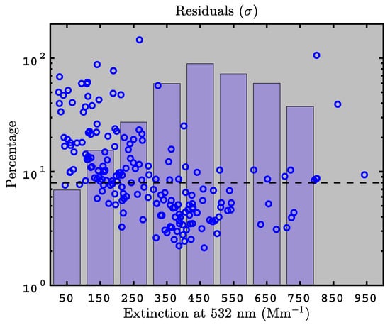
Figure 2.
Circles indicate GRASP residuals as a function of extinction for 195 successful PI-Neph measurements (using PSAP absorption measurements and a simulated solar zenith angle of ). The dashed line shows maximum residual allowed for Level 2 Aerosol Robotic Network (AERONET) retrievals (i.e., %). The bars indicate the percentage of retrievals that satisfy the % requirement in each extinction bin.
3.3. The Aerosol Samples
We tested a variety of different particles, as shown in Table 1. Many of the minerals that we tested were purchased from the Clay Minerals Society and shipped as clay powders or rock. We crushed and sieved the rocks to 44 m before testing. We also purchased Arizona Test Dust, hematite, and silica dust from Powder Technology Inc and illite-rich Arginotec NX from B + M Nottenkämper [72]. Two of our samples were collected from deserts in Senegal and Israel. The volcanic ash was collected from the Earth’s surface [73]. Soot of various sizes was obtained with a portable propane burner (Jing Ltd., miniCAST 4100). The size and organic carbon content of the soot was varied based upon the input flow of propane, air, and nitrogen to the burner [74].

Table 1.
285 different combinations of the following samples (internally and externally mixed), including humidified and dried runs of both PM and PM.
We also purchased several minerals from Natural Pigments, a company that specializes in the sale of artist pigments. Artist pigments are particularly convenient for testing iron oxides, as hematite and goethite are common commodities used by the art community to obtain reddish and yellowish hues. These natural substances are mined, separated from sand, ground to 50 m, and packaged for consumer use by the supplier. Pigments must contain at least 12% iron oxide to be labeled as an ocher, and French ochers typically contain about 20% iron oxide (per naturalpigments.com). Although there are many forms of hematite, only two forms are used as artist pigments: oolitic hematite and hematite rose. The iron content of the Blue Ridge Hematite that we tested is greater than 80%, according to the manufacturer specification sheet. Additional information about artist pigments is available at http://naturalpigments.com.
We used a flask and a shaker as a saltation mechanism to entrain the loose dry particles (dust, ash, and pigments) into our sample airstream, and limited the diameters of these particles to 1.0 or 2.5 m with a cyclone (i.e., PM and PM). Tests were usually run for 10–20 min to assure adequate temporal averaging. Although Table 1 only presents 43 aerosol species, we were able to obtain 285 independent samples by testing different particle sizes at ambient and high relative humidities (i.e., %) and by mixing different species. Mixing different samples also allowed us to test bimodal aerosol size distributions. We successfully processed PI-Neph data for 232 of the 285 samples, and the GRASP algorithm produced successful retrievals with residuals of less than 8% for about 90 of the samples. Most of the high-residual retrievals occurred when extinctions were less than 300 Mm (see Figure 2).
3.4. Simulating AERONET Scans at Different Solar Zenith Angles
The PI-Neph can obtain high angular resolution measurements at essentially all scattering angles between 4.5 and 175 degrees. The AERONET field instruments, on the other hand, have a different geometry with less angular resolution and range. The almuncantar scans used for the AERONET inversion products maintain a fixed elevation angle (equal to the solar elevation angle) and pause at 28 azimuth angles ranging from 3–180 degrees ([71], and https://aeronet.gsfc.nasa.gov/new_web/Documents/AERONETcriteria_final1_excerpt.pdf, Table 1). Consequently, the angular sampling varies with solar zenith angle and the maximum sampled scattering angle is equal to twice the solar zenith angle. High-quality Level 2 AERONET retrievals require < < in the Version 2 dataset.
This sampling issue is illustrated in Figure 3. The large squares in the upper two panels illustrate that the field instruments provide measurements over a smaller range of values when than when ; consequently, the retrievals are better constrained at large solar zenith angles. The lowest panel in Figure 3 presents the GRASP phase function when all available angles (1-degree averaging) are used for the retrieval. This high-resolution sampling is never available for AERONET or present-day satellite retrievals, but our results for 1-degree sampling are useful for understanding the utility of the PI-Neph as an in situ instrument.
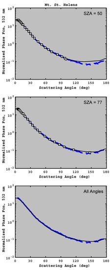
Figure 3.
Illustration of AERONET angular sampling for one of the test samples (volcanic ash from Mt. St. Helens, PM size cut). The small blue dots show the normalized phase function (532 nm wavelength) measured with the PI-Neph and averaged to one degree; these are identical in all three panels. The large squares in the top panel indicate subsampling used by AERONET instruments at a solar zenith angles of 50 degrees, while the squares in the middle panel indicate subsampling used by the AERONET instruments at a solar zenith angles of 77 degrees. The solid black lines in the top two panels show the phase function retrieved by the GRASP algorithm using the subsampled angles (squares). The black line in the bottom panel shows the retrieved phase function when the GRASP algorithm uses all available measurements (small blue dots).
Finally, we note that the AERONET team has recently added “hybrid scan” retrieval products to the Version 3 processing. The hybrid scan uses both the almucantar and principal plane (constant azimuth) geometries, which allows measurements over a wider range of scattering angles than can be achieved with the almucantar scan during periods of high sun. This decreases the minimum solar zenith angle required for Level 2 products from for the almucantar scan to for the hybrid scan (Brent Holben, personal communication). However, we do not analyze the hybrid scan sampling in this document.
4. Results
4.1. Single-Scatter Albedo
SSA () is defined as the ratio of scattering () to extinction (), but it may also be expressed in terms of aerosol absorption ():
SSA can be measured with in situ instrumentation located at the surface or on aircraft. Column retrievals of are available from satellite instrument products (e.g., Ozone Monitoring Instrument, Parasol) or the AERONET surface instruments. When represents extinction of the atmospheric column, or aerosol optical thickness (), the SSA links to absorption aerosol optical thickness ():
The AERONET retrievals of AAOD provide an important constraint for global aerosol models [26,34,35,75].
There are three ways to use Equation (3) to compare GRASP values with values derived by other instruments in Figure 1, and all three methods use the CAPS instrument for the extinction coefficient (represented by in Equation (3)). The first two methods use the PSAP and PASS instruments to determine the absorption coefficient (), and the third method uses the integrating nephelometer to determine the scattering coefficient (). We evaluate the performance of GRASP using all three methods, but the PI-Neph phase function used as input to GRASP is weighted with slightly different scattering coefficients for each comparison. So for instance, we set the absolute radiance I for GRASP to when comparing to , but we use when comparing to . This maintains a consistency of the radiance field and extinction coefficient with the appropriate in situ measurements.
Figure 4 provides a comparison of GRASP vs in situ for one of the above methods; here, the in situ was determined by Equation (3) using PSAP absorption measurements for and the CAPS extinction measurements for . Additionally, the PI-Neph data was subsampled with a simulated solar zenith angle of 50 for the GRASP input (e.g., see the top panel of Figure 3). The blue circles of Figure 4 indicate retrievals with residuals of 8% or less, which is consistent with AERONET Level 2 quality control at high . The white diamonds indicate retrievals with residuals greater than 8%. Blue circles in the left and right panels are identical, but the right panel has zoomed axes. Both panels indicate that the two datasets are highly correlated, with a correlation coefficient of for data that comply with the 8% residual restriction. The GRASP algorithm has a bias of +0.024 with respect to the in situ measurements when subject to the 8% residual restriction. Additional statistics for the blue circles are provided in Table 2.
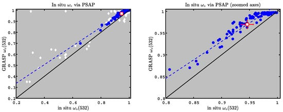
Figure 4.
Comparison of single-scatter albedo derived using GRASP to derived directly from PSAP absorption and CAPS extinction measurements. GRASP retrievals use scattering angles identical to data with solar zenith angles of 50 in the AERONET database. Blue circles indicate GRASP retrievals that have residuals of less than 8%, while white diamonds in the left panel indicate the additional scatter that occurs when residuals are not restricted. Red square is the mean value, and error bars represent two standard deviations of the mean. Data in the right panel is identical to blue circles in the left panel, but the axis ranges are different. In situ were determined using CAPS extinction measurements and PSAP absorption measurements. Solid lines are 1:1 and dashed blue lines correspond to linear regression of the blue circles; statistics are presented in Table 2.
Table 2.
Linear regression statistics for single-scatter albedo using different in situ measurement techniques. The first row of numbers corresponds to Figure 4, 4th and 7th rows correspond to Figure 5. Correlation coefficient is denoted by cc. Absolute bias and root mean square error , where represents the GRASP retrieval and represents the corresponding in situ measurement.
The high-residual retrievals in Figure 4 (white diamonds) still indicate a significant correlation with respect to the in situ measurements (), but the residual restriction of 8% for the blue circles clearly reduces the scatter and removes obvious outliers. We note that such outliers are not removed from standard AERONET Level 1.5 processing, so the user needs to use additional screening when analyzing Level 1.5 AERONET data to assure a quality analysis.
The right panel of Figure 4 focuses on the restricted data (i.e., residuals ≤8%). Here, we clearly see that the GRASP retrieval saturates before the in situ measurements, and GRASP seems to have less sensitivity to changes in than the in situ instrumentation when absorption is very low. That is, while exhibits a range of values from about 0.97 to 1. This is a consequence of the linearity and bias between the two measurements.
Our experiment also includes photo-acoustic and integrating nephelometer measurements that can be used with Equation (3) to compute ; scatter plots for these other two ways of computing are shown in Figure 5. The left panel of Figure 5 uses photo-acoustic absorption measurements and the plot is similar to the PSAP absorption measurements shown in Figure 4. The right panel compares GRASP to the calculated using integrating nephelometer measurements. Once again, we see a strong linearity between the GRASP and in situ values, but the integrating nephelometer produces the unphysical value for 19 of the 232 comparisons (8%), even under the ideal conditions of our laboratory experiment (i.e., minimum extinction of 12.3 Mm and ∼20-minute averaging time). This occurs because the scattering and extinction measurements produce comparable values when is small, so scattering/extinction ratios greater than one can be obtained when the noise of the two instruments are out of phase (i.e., when the scattering measurement has a high bias and the extinction measurement has a low bias). One might expect these abnormally large ratios of to occur at low extinctions, but the extinctions for these 19 points ranged from 28 Mm to 364 Mm. There are six points with , with extinctions ranging from 28 Mm to 110 Mm.
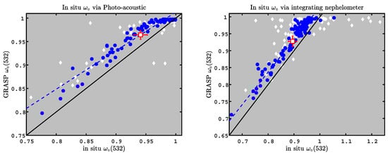
Figure 5.
Comparison of single-scatter albedo derived using GRASP to derived directly from in situ measurements. GRASP retrievals use scattering angles identical to data with solar zenith angles of 50 in the AERONET database. Left panel uses photo-acoustic absorption coefficients to determine , whereas the right panel uses the integrating nephelometer. Blue circles indicate GRASP retrievals that have residuals of less than 8%, while white diamonds indicate the additional scatter that occurs when residuals are not restricted. Red square is the mean value, and error bars represent two standard deviations of the mean. Solid lines are 1:1 and dashed blue lines correspond to linear regression of the blue circles; statistics presented in Table 2.
Statistics for all three methods of calculating are shown in Table 2 for two solar zenith angles as well as maximal sampling (i.e., 1-degree sampling). Table 2 shows that all three methods produce high correlation coefficients (0.916–0.976). The absolute bias () is less than +0.026 when the absorption coefficients are used to obtain , but reaches a value as high as +0.033 when scattering coefficients are used to determine . Absolute bias and error are nearly identical for simulated solar zenith angles of 50 and 77 (the same to within 0.001 for any method), indicating that solar zenith angle should not be a source of artifacts in the AERONET retrievals. The biases in Table 2 are consistent with uncertainties quoted for AERONET and in situ measurements [13,76]. We note that the GRASP retrieval of is always biased high of the in situ measurements, unlike aircraft comparisons that often show a low bias for AERONET retrievals [18]. We discuss this apparent discrepancy in Section 5.2.
Please note that increasing the angular resolution of the phase function measurements to 1 degree does not necessarily improve the SSA statistics in Table 2. This is because aerosol phase functions generally have a rather smooth angular dependence, so increasing the angular resolution of the measurements does not improve results over a subset of angles that capture the main angular features. Also note that the information content of the AERONET retrieval geometries has been extensively studied, and has led to the conclusion that 31 parameters (i.e., 22 radii, 8 real and imaginary refractive indices, and the percentage of spheres) can be uniquely retrieved from the standard AERONET measurements if a priori smoothness constraints on the size distribution and spectral dependence of the refractive index are applied [12,13,69,77].
4.2. Bistatic LiDAR Ratio
LiDAR ratio (or extinction-to-backscatter ratio) is an important parameter that is used to convert backscatter measurements to AOD for elastic LiDARs such as CALIPSO [78]. The LiDAR ratio is defined as:
where represents the normalized phase function at scattering angle , and represents the normalized phase function at . Since the SSA and phase function can be computed from the size distribution and complex refractive index, we can use the AERONET retrievals to compute column-effective LiDAR ratios for the atmosphere [69,79]. LiDAR ratio can also be measured with Raman LiDARs or high spectral resolution LiDARs (HSRLs) when these measurements are available (e.g., [80,81]). The LiDAR ratio is sensitive to particle size and complex refractive index [79,82]; consequently, different aerosol species exhibit different LiDAR ratios. That is, dust, pollution, and marine aerosols all have different LiDAR ratios, so LiDAR ratio can be used with other optical parameters to infer aerosol “type” [83,84].
Unfortunately, the PI-Neph does not measure the backscatter phase function at , so our experiment cannot provide measurements of the LiDAR ratio needed for elastic backscatter LiDARs. However, we can measure a bistatic LiDAR ratio by using instead of in Equation (5). Successful retrieval of the bistatic LiDAR ratio at improves confidence in the retrieval at , but it does not confirm the backscatter LiDAR ratio retrieval.
Results for 89 samples are shown in Figure 6; here, we used the PSAP absorption coefficients to determine and simulated solar zenith angles of 50 (left panel) or 77 (right panel). The circles correspond to retrievals with residuals ≤8% and are color-coded by the GRASP residual values. Linear regression statistics are shown in Table 3. Figure 6 indicates that individual GRASP-based calculations of can have substantial errors when , but the average value lands close to the 1:1 line (red square). The statistics presented in Table 3 also indicate that GRASP has substantial skill at computing for an ensemble of retrievals at this solar zenith angle (50): the correlation coefficient is cc = 0.714, the absolute bias is 1.79 sr, and the relative bias is 2%. The slope and intercept are 0.774 and 19.8 sr when , but these values improve to 1.004 and 7.55 sr when considering the 77 solar zenith angle. Further improvements in the correlation and absolute bias are achieved if 1-degree sampling is used for the GRASP retrievals.
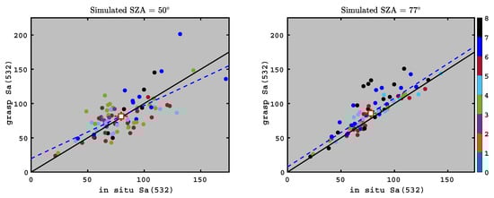
Figure 6.
Comparison of bistatic LiDAR ratio derived using the GRASP phase function to bistatic LiDAR ratio derived using PI-Neph phase function, both using a bistatic scattering angle of . Color code corresponds to retrieval residuals (%). Analysis in left panel uses a simulated solar zenith angle of 50 for the GRASP retrievals and the right panel uses a simulated solar zenith angle of 77. Solid lines are 1:1, dashed lines are linear regressions, and red squares are the mean of both methods; error bars represent two standard deviations of the mean. Regression statistics are provided in Table 3.
Table 3.
Linear regression statistics for bistatic LiDAR ratio at a backscatter angle of 173o and a wavelength of 532 nm, effective radius, average radius, effective variance, average standard deviation, and integrated volume of the size distributions. Analysis is restricted to retrievals with residuals of less than 8%. The in situ LiDAR ratio was computed using PSAP absorption measurements for in Equation (5) (i.e., ). The APS equivalent volume and were computed using variable dynamic shape factors (10% greater than ) or densities (10% less than ) for the conversion from aerodynamic size to equivalent volume size, as described in Section 4.3. Correlation coefficient is denoted by cc. Absolute bias , relative bias , and root mean square error , where represents the GRASP retrieval and represents the corresponding in situ measurement.
Interestingly, Table 3 indicates that the absolute and relative biases increase as increases from 50 to 77, which is unexpected. However, close inspection of Figure 6 indicates that there are many more points with residuals of 7–8% (black dots) at (right panel) than at (left panel). In fact, 60% of the retrievals right panel have residuals of 5–8% (), whereas only 44% of the retrievals in the left panel have residuals of 5–8% (). We also note that we can improve the statistics by filtering the analysis for residuals with values less than 5% (absolute and relative biases are reduced to 4 sr and 5%). Thus, it is probable that the higher quality residuals of the case are decreasing the absolute and relative biases with respect to the case. It is also worth mentioning that the case captures the variability better than the case (as shown by the slope and intercept), and that the case also has a better Taylor skill score [85]. The skill score for and 8% residual is 0.91, whereas the skill score for the comparison was only 0.85.
4.3. Converting Aerodynamic Size to Equivalent Spheres that Are Consistent with Extinction Measurements
We measured in situ size distributions with an aerodynamic particle sizer (APS) in our experiment. However, a direct comparison between the aerodynamic size distributions provided by the APS and the equivalent-volume size distributions provided by the GRASP retrievals is not possible because particle densities () and dynamic shape factors () are generally unknown. The equivalent volume diameter () is related to the aerodynamic diameter () by:
where is unit density, and are the Cunningham slip corrections associated with the aerodynamic and equivalent volume spheres (e.g., TSI application note APS-001, [86,87,88]). Cunningham correction factors vary with the Knudsen number (), which can be expressed as
where is the mean free path of the gas medium and d is the minor diameter for a spheroid particle. The mean free path of air at 1 standard atmosphere is 35 nm, which results in a maximum for the TSI APS (since m for APS measurements). Cunningham factors for various particle sizes and Knudsen numbers are listed in Table 17 of [89]; Knudsen numbers of 0.1 in that table indicate that ratio can vary by up to ∼10% from unity for randomly oriented spheroids with axis ratios up to infinity. Thus, we define as a parameter that has values similar to , and so relate the equivalent volume radius () to the aerodynamic radius () as
If is known, we can use simultaneous extinction and aerodynamic size measurements with Mie theory to determine the minimum value of necessary to achieve optical closure between aerodynamic size and extinction. This is illustrated in Figure 7; here, we measured the bulk aerosol density using a densimetry method, which is accurate to about ±10% [90]. The solid white line presents Mie computations of extinction for non-absorbing spherical aerosols using the APS size distribution with the measured density and a broad range of real refractive indices. The solid black line in the figure presents the CAPS extinction measurement for this sample. Since the solid white line is biased low of the solid black line for all reasonable values of the real refractive index, we know that non-absorbing Stokes-equivalent spheres (i.e., , , and ) cannot be used to compute the measured extinction. Furthermore, including absorbing particles in the Mie computations increases the bias, as evidenced by the brown line in Figure 7 where the imaginary refractive index is increased to . However, increasing the dynamic shape factor from 1.0 to 1.2 allows the Mie computations to replicate the measured extinction, as shown by the dashed white line. This indicates that results in an equivalent-volume size distribution that is consistent with the extinction measurements at the 532 nm wavelength. However, this figure only presents the 532 nm wavelength; implementing Mie computations with the aerodynamic size and all three CAPS wavelengths indicates that for this particular sample (other wavelengths not shown).
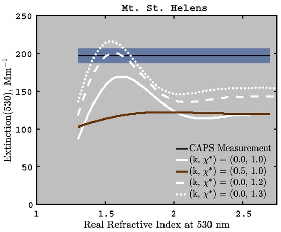
Figure 7.
Measured (black line) and computed extinctions of the Mt. St. Helens PM sample; shaded region covers % of measured value. Mie theory computations of volume equivalent sizes (white and brown lines) were processed using the measured aerodynamic size distribution, measured density (2.48 g-cm), and a wide range of real refractive indices. Each computed line has a specific imaginary refractive index (k) and dynamic shape factor () as noted in the legend. Intersections of computed white lines with the measured extinction line indicate that .
Likewise, if is unknown we can set and express Equation (8) as
In this case, we adjust to determine the maximum that is consistent with the measured size distribution and extinction. Results for both and for some samples are shown in Table 4. These parameters can be used to convert aerodynamic size distributions to equivalent-volume size distributions that are consistent with the CAPS extinction measurements. However, since and represent lower and upper bounds and do not precisely represent and , the resulting equivalent-volume size distributions are not necessarily correct. Nonetheless, using values of and guarantees size distributions that are consistent with the extinction measurements and provides an indication of whether the GRASP retrieval is consistent with the aerodynamic size measurements.
Table 4.
Bulk densities (, g-cm) measured using the densimetry technique and corresponding minimum dynamic shape factors () required to produce Mie theory extinctions from aerodynamic particle size for several of the tested samples with two different size cuts (PM or PM). Dried samples are presented in the left columns and samples humidified to 80+% are provided in the right column. Maximum (defined as , g-cm) that produce Mie theory extinctions from aerodynamic particle size are also shown. GRASP residuals for all samples are %, except for Brown Ocher and the hematites.
4.4. Statistical Comparison of Size Distributions
We are now able to compare the GRASP size distributions to the equivalent-volume size distributions inferred from the APS measurements. We begin by presenting the respective size distributions for a single run in Figure 8. Here, we see that both the GRASP and APS methods indicate similar peak mode radii, but that GRASP infers a lower peak volume concentration and a significantly higher mode width than the APS measurement. We found this type of behavior to be rather typical of our observations, as discussed below.
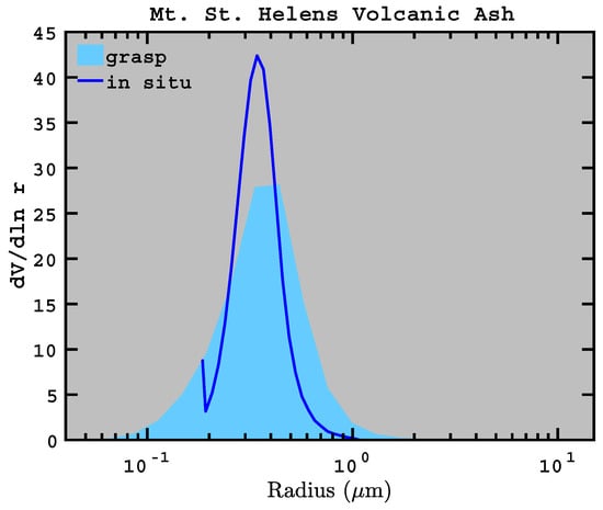
Figure 8.
Comparison of retrieved size distribution (GRASP) with APS measurements of equivalent volume spheres for dry PM volcanic ash that was erupted from Mount St. Helens. The GRASP size distribution was obtained using a simulated solar zenith angle of 50, and the APS aerodynamic size measurements were converted to equivalent volume spheres using a dynamic shape factor of ; this is the minimum -value consistent with Mie theory and extinction measurements (as discussed in Section 4.3). Relative bias of the GRASP effective variance with respect to APS measurements for this case is 2.94, which is close to the average variance bias of 2.80 shown in Table 3 at .
To compare multiple size distributions, though, we need a simple way of characterizing the size distributions with a couple of parameters. The effective radii () and effective widths () of size distributions are recognized as the best parameters for determining the radiative impact of particle size distributions (e.g., [66,91]):
and
Note the spuriously high value of in the lowest-radius bin of the in situ measurements in Figure 8, which often occurred during the STEAR experiment. This spurious behavior occurs because the lowest-radius bin captures all particles smaller than a certain size; consequently, this bin has a larger bin width than all the other bins. Therefore, particle volumes cannot be computed accurately for the particles in that bin, so we do not include the first APS bin in the effective radii and effective variance calculations of Equations (10) and (11). We also adjust the lower integration limit of the GRASP size distributions to match the in situ lower limit (for Figure 8, this is 0.19 m) so that both methods cover the same range of particle sizes.
We compare GRASP effective radii and variances (with a simulated ) to equivalent-volume effective radii and variances in Figure 9 and Figure 10, using or to convert aerodynamic size to equivalent volume size. Linear regression statistics for the effective radius and effective variance comparisons are shown in Table 3 for , , and 1-degree sampling. Here we see that the absolute bias of the effective radius ranges from to m and that the absolute relative bias is always less than 22%. (Please note that the subsampled GRASP retrievals that simulate AERONET produce lower biases than the 1-deg sampling.)
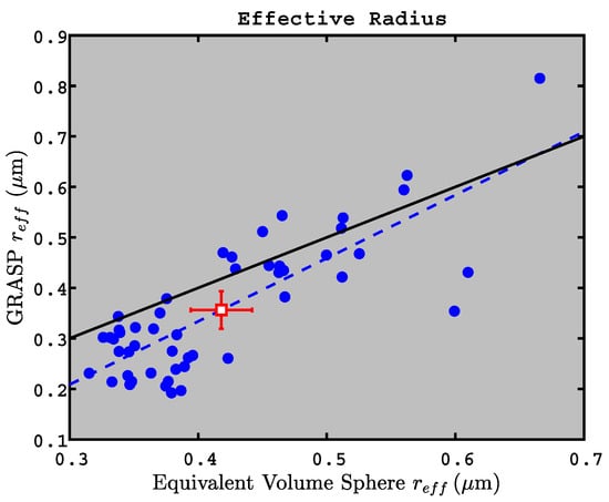
Figure 9.
GRASP effective radius (subsampled to an equivalent solar zenith angle of 50) vs. APS equivalent-volume effective radius using variable dynamic shape factors or densities for the conversion from aerodynamic size to equivalent volume size. Red square and error bars represent means and two standard deviations of the means for the blue points. Solid line is 1:1 and dashed line represents linear regression; see Table 3 for regression statistics.
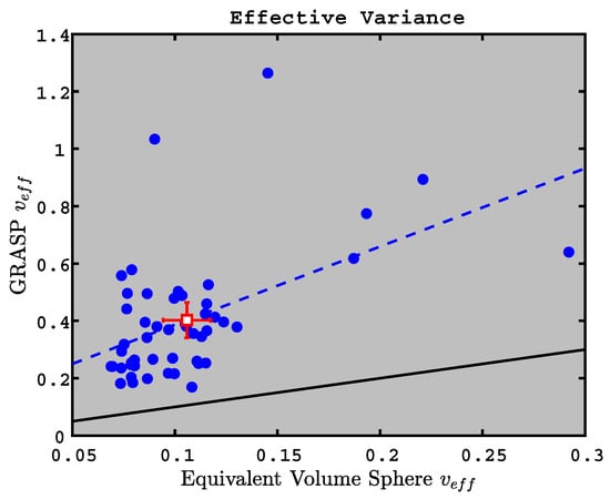
Figure 10.
GRASP effective variance (subsampled to an equivalent solar zenith angle of 50) vs. APS equivalent volume variance using variable dynamic shape factors or densities for the conversion from aerodynamic size to equivalent volume size. Red square and error bars represent means and two standard deviations of the means for the blue points. Solid line is 1:1 and dashed line represents linear regression; see Table 3 for regression statistics.
The GRASP size distributions are significantly wider than the APS values, however, and Table 3 indicates that the GRASP has relative biases of 280–324% for our three sampling schemes. Both AERONET retrievals and in situ measurements have significant uncertainties regarding variances, but the variance biases that we measured seem to be larger than those found during field campaign comparisons of AERONET with in situ measurements [92,93,94,95]. We note that the variances retrieved with GRASP are quite stable when using the a priori smoothness constraints that we have chosen, and that when those constraints are relaxed, the size distributions exhibit unrealistic oscillations. This means that there are smoothing effects associated with the fundamentals of light scattering by ensembles of particles, and a fundamental bias to larger variances for the GRASP technique may indeed exist. However, the in situ methods also rely upon several assumptions (especially for non-spherical particles) and this contributes to the bias as well (see, for example, Reid et al., 2003, for a discussion about measurement assumptions required for in situ observations of irregularly shaped particles [92]).
We also compare the total aerosol volumes (or integrated size distributions), which is an underused parameter in the AERONET database. Aerosol volume is important because it provides a link to the mass-based emissions that are the starting point for all aerosol transport models. Although many aerosol transport models produce the correct , they do not necessarily produce the correct column mass load. (Correct modeled with incorrect column mass load occurs when size distribution assumptions in the model are incorrect). The AERONET aerosol volumes, on the other hand, are constrained by and the scattered radiation field. Taken together, AERONET and aerosol volume offer a pair of constraints that could improve the size distribution and refractive index assumptions in the models. Modelers who can reliably produce the AERONET aerosol volumes can argue that their modeled column aerosol mass is consistent with the measured radiation field.
The results of the aerosol volume comparison are shown in Figure 11 and statistics are provided in Table 3. The correlation coefficient is greater than 0.84 and the relative bias is less than 16% for both simulated solar zenith angles (50 and 77). This indicates that the GRASP retrieval provides reliable aerosol volume concentrations when configured for the AERONET viewing geometries, and that the integrated size distributions can be used with confidence as a validation parameter for aerosol transport model simulations.
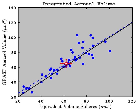
Figure 11.
Total aerosol volume for GRASP and APS equivalent volume spheres. GRASP retrievals subsampled to an equivalent solar zenith angle of 50; APS sphere sizes determined using or . Red square and error bars represent means and two standard deviations of the means for the blue points. Solid line is 1:1 and dashed line represents linear regression; see Table 3 for regression statistics.
5. Discussion
5.1. GRASP Imaginary Refractive Index as an Indicator of Aerosol Absorption
The imaginary refractive index of a material is an intrinsic parameter that is directly related to the bulk absorption coefficient (e.g., [96,97,98]). We test the ability of the GRASP algorithm to quantify aerosol absorption by comparing the GRASP imaginary refractive indices to in situ SSA measurements (expecting a strong anti-correlation). We tested 89 samples that included various proportions of soot and fullerene mixed with ammonium sulfate, ammonium nitrate, and mineral dust, adjusting the carbonaceous fraction to achieve SSAs between 0.78 and 0.98. We found the GRASP imaginary refractive index to be highly anti-correlated with the in situ SSA (), as shown in Figure 12. We conclude that the GRASP imaginary index can be used to determine bulk aerosol absorption properties that are consistent with in situ SSA measurements.
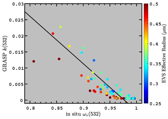
Figure 12.
Imaginary refractive index for 89 samples that have residuals 8%, plotted against single-scatter albedo (measured with CAPS extinction and PSAP absorption). Data are color-coded with the effective radii of equivalent volume spheres (EVSs) computed from aerodynamic size using the method outlined in Section 4.3 to obtain dynamic shape factors. A simulated solar zenith angle of was used for the GRASP imaginary index retrieval. Solid line is a linear regression with correlation coefficient of . Please note that the color code indicates that tends to decrease with respect to for a given k-value.
The advantage of using refractive index to understand inherent aerosol properties over SSA is that the refractive index does not depend upon the size of the particles. That is, even though SSA is often used as an indicator of intrinsic aerosol absorption, it is not a truly intrinsic aerosol parameter. This is because the SSA depends upon the size of the particles as well as the absorption. The variability of SSA with particle size also manifests itself in Figure 12, which shows significant spread in SSA for a given imaginary refractive index; the color code in that figure indicates that large particles generally have lower SSAs than the small particles. Since any internal mixture of aerosol components has a certain imaginary refractive index, one must also conclude that a range of SSAs also occur for a given aerosol mixture. This confounds attempts to characterize aerosol composition (e.g., the relative contribution of carbonaceous or dust particles) solely based on the AERONET SSA retrievals.
5.2. AERONET Absorption bias
Figure 4 and Figure 5, and Table 2 indicate that the SSA inferred by the GRASP/AERONET algorithm has a high bias of 0.024–0.036 when compared to in situ measurements, indicating that the AERONET algorithm might not be capturing enough absorption in the global data product. On the contrary, Andrews et al., 2017 [18] found a low bias of AERONET retrievals with respect to in situ aircraft measurements, especially at low s. AERONET retrievals of are also biased low of global aerosol models as well [26,34]. Since AERONET is biased low of both in situ measurements and global aerosol models, there is a concern that the AERONET retrievals might be indicating too much absorption [35].
However, most (if not all) comparisons of aerosol absorption with AERONET retrievals include Level 1.5 retrievals with (in addition to the high-quality Level 2.0 retrievals that are not available at low ). These low retrievals are known to have substantially more noise than the Level 2.0 retrieval products, but the low are still used because their omission would skew the average to inappropriately high values. The rationale is that the average values of the Level 1.5 retrievals at low might be correct, even though individual retrievals can be unrealistic. However, Bond et al. 2013 [35] point out that the AERONET retrievals are capped at (see their Appendix B), and that the resulting distribution of at low is not Gaussian. Consequently, this causes a low bias in the retrieved .
We are unable to address the low issue with this study. The GRASP/AERONET retrievals presented in Section 4 have the benefit of strong signal-to-noise ratios (SNRs) that are not always possible to obtain with field measurements. Please note that the minimum extinction coefficient with an acceptable residual (i.e., %) in Figure 2 is 45 Mm, and the median extinction of the data points with acceptable residuals is 388 Mm. We also note that the median PSAP absorption coefficient consistent with our residual requirement is 14.1 Mm, and 98% of the absorption coefficients are greater than 1 Mm. Thus, the aerosol loading in our experiment is substantial enough to quantify using both the GRASP algorithm and the in situ instrumentation, but we cannot claim to have evaluated the AERONET retrievals in circumstances with low AOD. Indeed, a low-AOD assessment of the AERONET algorithm is not possible using our experimental apparatus, since instrument sensitivity is so important at low SNR and our instrumentation is different than the AERONET field instruments.
5.3. Caveats
The successful results shown here are “necessary but not sufficient” proof that the AERONET retrievals (or any other aerosol retrieval) works correctly. That is, our experiment fulfills some of the validation requirements for column aerosol retrievals, but not all of them; this is because the geometry of our experiment is not an exact imitation of the atmosphere or the AERONET instruments. The sensitivity and calibration of our in situ measurements is different than the AERONET Cimels, and our experiment does not suffer complexities associated with a multiple-scattering atmosphere that could possibly contain clouds [99,100]. Modern radiative transfer models are sophisticated enough that computation of clear-sky radiances can be done with confidence, though, [101,102], so the lack of a multiple-scattering atmosphere in these comparisons is no longer a major issue.
Additionally, there is a wavelength mismatch between the PI-Neph (0.473, 0.532, and 0.671 m) and the AERONET instrument (0.440, 0.670, 0.870, 1.020 m), and a particle size discrepancy between our experiment (max diameter ∼2.5 m) and the AERONET retrievals (sensitive up to 15 m radius). Admittedly, we have not proven anything about the ability to retrieve coarse mode radii larger than ∼1.25 m than with this experiment—that must be left to future experiments using longer wavelengths and larger inlets. However, the wavelength range that we are using provides plenty of sensitivity to the aerosol distributions observed in our experiment.
Finally, our in situ measurements were performed at a static location and benefited from high frequency sampling that was averaged over 10–20 min to vastly improve SNRs; atmospheric remote sensing does not have this luxury because of relatively slow scan times for the AERONET instruments and the rapid speed of the satellite instruments. Satellite retrievals are also susceptible to rapidly changing surface albedos as the spacecraft moves over land.
6. Conclusions
We have created a laboratory experiment to evaluate the fidelity of the core AERONET retrieval algorithm using the GRASP retrieval algorithm. That is, we measured the extinction and angular dependence of scattering of real aerosols while simultaneously measuring aerosol microphysical and optical properties with conventional in situ techniques. Importantly, we subsampled our scattering measurements to match AERONET’s sampling at solar zenith angles of 50 and 77 (this brackets the range of allowed for Level 2.0 AERONET almucantar scans), and limited our analysis to retrievals with residuals less than 8% in order to maintain consistency with AERONET Level 2.0 processing. We then compared the aerosol microphysical and optical properties inferred by the GRASP algorithm to the same properties measured with in situ instruments. We contend that this is a more robust method for determining retrieval algorithm performance than theoretical sensitivity studies, which require simplified aerosol microphysics to compute the scattered radiation fields. Overall, we generally found positive results.
We found that the GRASP-retrieved SSA () has a high absolute bias of about 0.024 with respect to in situ measurements of absorption and extinction. (The bias is slightly higher when the in situ measurements are based upon scattering and extinction, but this in situ method sometimes indicated , casting doubt upon the reliability of this approach.) This result contrasts the low bias that was observed when AERONET was compared to flight measurements [18], but we attribute the low bias of [18] to the low AODs that dominated those measurements. We also note that the GRASP-retrieved imaginary refractive index is highly correlated with the in situ SSA (), as expected.
The retrieved bistatic LiDAR ratio at a scattering angle of has an absolute high bias of 1.79 to 7.89 sr and a relative bias of 2–10% with respect to CAPS extinction and PI-Neph scattering measurements, depending upon the simulated solar zenith angle.
The effective radius of the retrieved size distributions has a low absolute bias of 0.05 m and a low relative bias of 13% with respect to aerodynamic particle size measurements adjusted to determine the EVS radii. The retrieved size distributions are significantly wider than the aerodynamic measurements, however, indicating a relative bias of up to 280% for the effective variance. The retrieved size distributions have maximums at lower values than the EVS, though, so that the total aerosol volume of the simulated AERONET size distributions are biased high of the EVS by less than 16%.
Perhaps the most significant feature of this work is that the phase functions are generated with real aerosols, rather than using theoretical values from a forward scattering model. Forward scattering computations are valuable for understanding the scattering properties of aerosols, but computational speeds are slow for complicated morphologies; consequently, the scope of non-spherical scattering studies is necessarily limited. Although our apparatus cannot mimic all aspects of the instruments and measurements associated with actual remote sensing, the technique presented here is an important component of a multi-pronged effort for validating column aerosol retrievals in a statistically robust manner (in addition to in situ measurements and model sensitivity studies). That is, if a retrieval algorithm cannot provide accurate microphysical properties for real aerosols using data from a controlled laboratory experiment, then it certainly will not be able to provide accurate results based upon atmospheric radiance measurements. Given the minuscule cost of a laboratory experiment in comparison to the cost of a satellite mission, laboratory experiments with real particle populations that mimic future satellite viewing geometries should be an integral part of any aerosol remote sensing project.
Supplementary Materials
The GRASP algorithm is publicly available at http://www.grasp-open.com/. Data for the in situ measurements that are maintained by the Langley Aerosol Group (LARGE) are available at https://science.larc.nasa.gov/large/data.html.
Author Contributions
Conceptualization and funding acquisition, G.L.S., L.D.Z., A.J.B., B.E.A., J.V.M., O.D. and Y.D.; methodology, G.L.S., L.D.Z., A.J.B., B.E.A. and J.V.M.; GRASP software, O.D., F.D., D.F. and T.L.; other software, M.S.; validation, Y.D.; formal analysis, G.L.S., W.R.E., L.D.Z., A.J.B. and A.R.; investigation, W.R.E., L.D.Z., A.J.B., A.R.-L. and R.M.; resources, G.L.S., A.R. and Y.D.; data curation, W.R.E., L.D.Z., A.J.B., A.R. and M.S.; writing—original draft preparation, G.L.S. and W.R.E.; writing—review and editing, G.L.S., W.R.E., A.J.B., D.F. and R.H.M.; visualization, G.L.S.; supervision, G.L.S., B.E.A., J.V.M. and O.D.; project administration, G.L.S., W.R.E., L.D.Z., A.J.B., A.R.-L. and J.V.M.
Funding
This material in this work is supported by the National Aeronautics and Space Administration through the Science Mission Directorate’s Earth Science Division, Program Element A.14: Atmospheric Composition Laboratory Research. Y. Derimian, O. Dubovik. F. Ducos and T. Lapyonok appreciate support by the CaPPA project (Chemical and Physical Properties of the Atmosphere), which is funded by the French National Research Agency (ANR) through the PIA (Programme d’Investissement d’Avenir) under contract <<ANR-11-LABX-0005-01>> and by the Regional Council <<Hauts-de-France>> and the <<European Funds for Regional Economic Development>> (FEDER).
Acknowledgments
We appreciate the efforts of Bobby Martin and Joel Alexa for processing and analyzing mineral rocks at NASA LaRC, and Matthias Schuhbauer of B + M Nottenkämper for providing the Arginotec NX sample. We also appreciate the efforts of those who collected and shared volcanic ash samples, including Nickolay Krotkov, H. Olafsson, U. Shumann, and Philip DeCola.
Conflicts of Interest
The authors declare no conflict of interest.
References
- Tanré, D.; Kaufman, Y.; Herman, M.; Mattoo, S. Remote sensing of aerosol properties over oceans using the MODIS/EOS spectral radiances. J. Geophys. Res. 1997, 102, 16971–16988. [Google Scholar] [CrossRef]
- Remer, L.; Kaufman, Y.; Tanre, D.; Mattoo, S.; Chu, D.A.; Martins, J.; Li, R.R.; Ichoku, C.; Levy, R.; Kleidman, R.; et al. The MODIS Aerosol Algorithm, Products, and Validation. J. Atmos. Sci. 2005, 62, 947–973. [Google Scholar] [CrossRef]
- Levy, R.; Mattoo, S.; Munchak, L.; Sayer, A.; Patadia, F.; Hsu, N. The Collection 6 MODIS aerosol products over land and ocean. Atmos. Meas. Tech. 2013, 6, 2989–3034. [Google Scholar] [CrossRef]
- Lyapustin, A.; Wang, Y.; Laszlo, I.; Kahn, R.; Korkin, S.; Remer, L.A.; Levy, R.; Reid, J. Multiangle implementation of atmospheric correction (MAIAC): 2. Aerosol algorithm. J. Geophys. Res. 2011, 116. [Google Scholar] [CrossRef]
- Diner, D.; Bruegge, C.; Martonchik, J.; Ackerman, T.; Davies, R.; Gerstl, S.; Gordon, H.; Sellers, P.; Clark, J.; Daniels, J.; et al. MISR: A Multiangle Imaging SpectroRadiometer for Geophysical and Climatological Research from Eos. IEEE Trans. Geosci. Remote Sens. 1989, 27, 200–214. [Google Scholar] [CrossRef]
- Deschamps, P.Y.; Brèon, F.M.; Leroy, M.; Podaire, A.; Bricaud, A.; Buriez, J.C.; Sèze, G. The POLDER Mission: Instrument Characteristics and Scientific Objectives. IEEE Trans. Geosci. Remote Sens. 1994, 32, 598–615. [Google Scholar] [CrossRef]
- Martonchik, J.; Diner, D.; Kahn, R.; Ackerman, T.; Verstraete, M.; Pinty, B.; Gordon, H. Techniques for the Retrieval of Aerosol Properties Over Land and Ocean Using Multiangle Imaging. IEEE Trans. Geosci. Remote Sens. 1998, 36, 1212–1227. [Google Scholar] [CrossRef]
- Hasekamp, O.; Landgraf, J. Retrieval of aerosol properties over land surfaces: Capabilities of multiple-viewing-angle intensity and polarization measurements. Appl. Opt. 2007, 46, 3332–3344. [Google Scholar] [CrossRef] [PubMed]
- Yu, H.; Quinn, P.; Feingold, G.; Remer, L.; Kahn, R.; Chin, M.; Schwartz, S. Remote Sensing and In Situ Measurements of Aerosol Properties, Burdens, and Radiative Forcing. In Atmospheric Aerosol Properties and Climate Impacts; A Report by the U.S. Climate Change Science Program and the Subcommittee on Global Change Research; National Aeronautics and Space Administration: Washington, DC, USA, 2009. [Google Scholar]
- Tanré, D.; Bréon, F.; Deuzé, J.; Dubovik, O.; Ducos, F.; Franois, P.; Goloub, P.; Herman, M.; Lifermann, A.; Waquet, F. Remote sensing of aerosols by using polarized, directional and spectral measurements within the A-Train: The PARASOL mission. Atmos. Meas. Tech. 2011, 4, 1383–1395. [Google Scholar] [CrossRef]
- Holben, B.; Eck, T.; Slutsker, I.; Tanre, D.; Buis, J.; Setzer, A.; Vermote, E.; Reagan, J.; Kaufman, Y.; Nakajima, T.; et al. AERONET—A federated instrument network and data archive for aerosol characterization. Remote Sens. Environ. 1998, 66, 1–16. [Google Scholar] [CrossRef]
- Dubovik, O.; King, M. A flexible inversion algorithm for retrieval of aerosol optical properties from sun and sky radiance measurements. J. Geophys. Res. 2000, 105, 20673–20696. [Google Scholar] [CrossRef]
- Dubovik, O.; Smirnov, A.; Holben, B.; King, M.; Kaufman, Y.; Eck, T.; Slutsker, I. Accuracy assessments of aerosol optical properties retrieved from Aerosol Robotic Network (AERONET) sun and sky radiance measurements. J. Geophys. Res. 2000, 105, 9791–9806. [Google Scholar] [CrossRef]
- Holben, B.; Tanre, D.; Smirnov, A.; Eck, T.; Slutsker, I.; Abuhassan, N.; Newcomb, W.; Schafer, J.; Chatenet, B.; Lavenu, F.; et al. An emerging ground-based aerosol climatology: Aerosol optical depth from AERONET. J. Geophys. Res. 2001, 106, 12067–12097. [Google Scholar] [CrossRef]
- Thomas, G.; Stamnes, K. Radiative Transfer in the Atmosphere and Ocean; Cambridge University Press: Cambridge, UK, 1999. [Google Scholar]
- Giles, D.; Holben, B.; Tripathi, S.; Eck, T.; Newcomb, W.; Slutsker, I.; Dickerson, R.; Thomspon, A.; Mattoo, S.; Wang, S.H.; et al. Aerosol properties over the Indo-Gangetic Plain: A mesoscale perspective from the TIGERZ experiment. J. Geophys. Res. 2011, 116. [Google Scholar] [CrossRef]
- Holben, B.N.; Kim, J.; Sano, I.; Mukai, S.; Eck, T.F.; Giles, D.M.; Schafer, J.S.; Sinyuk, A.; Slutsker, I.; Smirnov, A.; et al. An overview of mesoscale aerosol processes, comparisons, and validation studies from DRAGON networks. Atmos. Chem. Phys. 2018, 18, 655–671. [Google Scholar] [CrossRef]
- Andrews, E.; Ogren, J.; Kinne, S.; Samset, B. Comparison of AOD, AAOD and column single scattering albedo from AERONET retrievals and in situ profiling measurements. Atmos. Chem. Phys. 2017, 17, 6041–6072. [Google Scholar] [CrossRef]
- Diner, D.; Bruegge, C.; Martonchik, J.; Bothwell, G.; Danielson, E.; Floyd, E.; Ford, V.; Hovland, L.; Jones, K.; White, M. A Multiangle Imaging SpectroRadiometer for Terrestrial Remote Sensing from the Earth Observing System. Int. J. Imaging Syst. Technol. 1991, 3, 92–107. [Google Scholar] [CrossRef]
- Winker, D.; Pelon, J.; Coakley, J.; Ackerman, S.; Charlson, R.; Colarco, P.; Flamant, P.; Fu, Q.; Hoff, R.; Kittaka, C.; et al. The CALIPSO Mission: A global 3D View of Aerosols and Clouds. Bull. Am. Meteorol. Soc. 2010, 91, 1211–1229. [Google Scholar] [CrossRef]
- Hodzic, A.; Chepfer, H.; Vautard, R.; Chazette, P.; Beekmann, M.; Bessagnet, B.; Chatenet, B.; Cuesta, J.; Drobinski, P.; Goloub, P.; et al. Comparison of aerosol chemistry transport model simulations with lidar and Sun photometer observations at a site near Paris. J. Geophys. Res. 2004, 109. [Google Scholar] [CrossRef]
- Reddy, M.; Boucher, O.; Bellouin, N.; Schulz, M.; Balkanski, Y.; Dufresne, J.L.; Pham, M. Estimates of global multicomponent aerosol optical depth and direct radiative perturbation in the Laboratoire de Meteorologie Dynamique general circulation model. J. Geophys. Res. 2005, 110. [Google Scholar] [CrossRef]
- Kinne, S.; Schulz, M.; Textor, C.; Guibert, S.; Balkanski, Y.; Bauer, S.; Berntsen, T.; Berglen, T.; Boucher, O.; Chin, M.; et al. An AeroCom initial assessment – optical properties in aerosol component modules of global models. Atmos. Chem. Phys. 2006, 6, 1–20. [Google Scholar] [CrossRef]
- Stier, P.; Seinfeld, J.; Kinne, S.; Boucher, O. Aerosol absorption and radiative forcing. Atmos. Chem. Phys. 2007, 7, 5237–5261. [Google Scholar] [CrossRef]
- Chin, M.; Diehl, T.; Dubovik, O.; Eck, T.; Holben, B.; Sinyuk, A.; Streets, D. Light absorption by pollution, dust, and biomass burning aerosols: A global model study and evaluation with AERONET measurements. Ann. Geophys. 2009, 27, 3439–3464. [Google Scholar] [CrossRef]
- Koch, D.; Schulz, M.; Kinne, S.; McNaughton, C.; Spackman, J.; Balkanski, Y.; Bauer, S.; Berntsen, T.; Bond, T.; Boucher, O.; et al. Evaluation of black carbon estimations in global aerosol models. Atmos. Chem. Phys. 2009, 9, 9001–9026. [Google Scholar] [CrossRef]
- Kinne, S.; Lohmann, U.; Feichter, J.; Schulz, M.; Timmreck, C.; Ghan, S.; Easter, R.; Chin, M.; Ginoux, P.; Takemura, T.; et al. Monthly averages of aerosol properties: A global comparison among models, satellite data, and AERONET ground data. J. Geophys. Res. 2003, 108. [Google Scholar] [CrossRef]
- Loría-Salazar, S.; Arnott, W.; Moosmüller, H. Accuracy of near-surface aerosol extinction determined from columnar aerosol optical depth measurements in Reno, NV, USA. J. Geophys. Res. Atmos. 2014, 119, 11355–11374. [Google Scholar] [CrossRef]
- Pierce, A.; Loría-Salazar, S.; Holmes, H.; Gustin, M. Investigating horizontal and vertical pollution gradients in the atmosphere associated with an urban location in complex terrain, Reno, Nevada, USA. Atmos. Environ. 2019, 196, 103–117. [Google Scholar] [CrossRef]
- Dubovik, O.; Holben, B.; Eck, T.; Smirnov, A.; Kaufman, Y.; King, M.; Tanre, D.; Slutsker, I. Variability of absorption and optical properties of key aerosol types observed in worldwide locations. J. Atmos. Sci. 2002, 59, 590–608. [Google Scholar] [CrossRef]
- Levy, R.C.; Remer, L.A.; Dubovik, O. Global aerosol optical properties and application to Moderate Resolution Imaging Spectroradiometer aerosol retrieval over land. J. Geophys. Res. 2007, 112. [Google Scholar] [CrossRef]
- Colarco, P.; da Silva, A.; Chin, M.; Diehl, T. Online simulations of global aerosol distributions in the NASA GEOS-4 model and comparisons to satellite and ground-based aerosol optical depth. J. Geophys. Res. 2010, 115. [Google Scholar] [CrossRef]
- Russell, P.; Kacenelenbogen, M.; Livingston, J.; Hasekamp, O.; Burton, S.; Schuster, G.; Johnson, M.; Knobelspiesse, K.; Redemann, J.; Ramachandran, S.; et al. A multiparameter aerosol classification method and its application to retrievals from spaceborne polarimetry. J. Geophys. Res. 2014, 119. [Google Scholar] [CrossRef]
- Sato, M.; Hansen, J.; Koch, D.; Lacis, A.; Ruedy, R.; Dubovik, O.; Holben, B.; Chin, M.; Novakov, T. Global atmospheric black carbon inferred from AERONET. Proc. Natl. Acad. Sci. USA 2003, 100, 6319–6324. [Google Scholar] [CrossRef] [PubMed]
- Bond, T.; Doherty, S.; Fahey, D.; Forster, P.; Berntsen, T.; DeAngelo, B.; Flanner, M.; Ghan, S.; Kärcher, B.; Koch, D.; et al. Bounding the role of black carbon in the climate system: A scientific assessment. J. Geophys. Res. 2013, 118, 1–173. [Google Scholar] [CrossRef]
- Dubovik, O.; Herman, M.; Holdak, A.; Lapyonok, T.; Tanré, D.; Deuzé, J.; Ducos, F.; Sinyuk, A.; Lopatin, A. Statistically optimized inversion algorithm for enhanced retrieval of aerosol properties from spectral mult-angle polarimetric satellite observations. Atmos. Meas. Tech. 2011, 4, 975–1018. [Google Scholar] [CrossRef]
- Dubovik, O.; Lapyonok, T.; Litvinov, P.; Herman, M.; Fuertes, D.; Ducos, F.; Lopatin, A.; Chaikovsky, A.; Torres, B.; Derimian, Y.; et al. GRASP: A versatile algorithm for characterizing the atmosphere. SPIE Newsroom 2014. [Google Scholar] [CrossRef]
- Kokhanovsky, A.; Davis, A.; Cairns, B.; Dubovik, O.; Hasekamp, O.; Sano, I.; Mukai, S.; Rozanov, V.; Litvinov, P.; Lapyonok, T.; et al. Space-based remote sensing of atmospheric aerosols: The multi-angle spectro-polarimetric frontier. Earth-Sci. Rev. 2015, 145, 85–116. [Google Scholar] [CrossRef]
- Popp, T.; de Leeuw, G.; Bingen, C.; Brühl, C.; Capelle, V.; Chedin, A.; Clarisse, L.; Dubovik, O.; Grainger, R.; Griesfeller, J.; et al. Development, Production and Evaluation of Aerosol Climate Data Records from European Satellite Observations (Aerosol_cci). Remote Sens. 2016, 8, 421. [Google Scholar] [CrossRef]
- Benavent-Oltra, J.; Román, R.; Granados-Muñoz, M.J.; Pérez-Ramírez, D.; Ortiz-Amezcua, P.; Denjean, C.; Lopatin, A.; Lyamani, H.; Torres, B.; Guerrero-Rascado, J.L.; et al. Comparative assessment of GRASP algorithm for a dust event over Granada (Spain) during ChArMEx-ADRIMED 2013 campaign. Atmos. Meas. Tech. 2017, 10. [Google Scholar] [CrossRef]
- Román, R.; Torres, B.; Fuertes, D.; Cachorro, V.; Dubovik, O.; Toledano, C.; Cazorla, A.; Barreto, A.; Bosch, J.; Lapyonok, T.; et al. Remote sensing of lunar aureole with a sky camera: Adding information in the nocturnal retrieval of aerosol properties with GRASP code. Remote Sens. Environ. 2017, 196, 238–252. [Google Scholar] [CrossRef]
- Tsekeri, A.; Lopatin, A.; Amiridis, V.; Marinou, E.; Igloffstein, J.; Siomos, N.; Solomos, S.; Kokkalis, P.; Engelmann, R.; Baars, H.; et al. GARRLiC and LIRIC: Strengths and limitations for the characterization of dust and marine particles along with their mixtures. Atmos. Meas. Tech. 2017, 10. [Google Scholar] [CrossRef]
- Chen, C.; Dubovik, O.; Henze, D.; Lapyonok, T.; Chin, M.; Ducos, F.; Litvinov, P.; Huang, X.; Li, L. Retrieval of desert dust and carbonaceous aerosol emissions over Africa from POLDER/PARASOL products generated by the GRASP algorithm. Atmos. Chem. Phys. 2018, 18, 12551–12580. [Google Scholar] [CrossRef]
- Lopatin, A.; Dubovik, O.; Chaikovsky, A.; Goloub, P.; Lapyonok, T.; Tanré, D.; Litvinov, P. Enhancement of aerosol characterization using synergy of lidar and sun—Photometer coincident observations: The GARRLiC algorithm. Atmos. Meas. Tech. 2013, 6, 2065–2088. [Google Scholar] [CrossRef]
- Espinosa, W.; Remer, L.A.; Dubovik, O.; Ziemba, L.; Beyersdorf, A.; Orozco, D.; Schuster, G.; Lapyonok, T.; Fuertes, D.; Martins, J. Retrievals of aerosol optical and microphysical properties from Imaging Polar Nephelometer scattering measurements. Atmos. Meas. Tech. 2017, 10, 811–824. [Google Scholar] [CrossRef]
- Torres, B.; Dubovik, O.; Fuertes, D.; Schuster, G.; Cachorro, V.; Lapyonok, T.; Goloub, P.; Blarel, L.; Barreto, A.; Mallet, M.; et al. Advanced characterisation of aerosol size properties from measurements of spectral optical depth using the GRASP algorithm. Atmos. Meas. Tech. 2017, 10, 3743–3781. [Google Scholar] [CrossRef]
- Derimian, Y.; Dubovik, O.; Huang, X.; Lapyonok, T.; Litvinov, P.; Kostinski, A.; Dubuisson, P.; Ducos, F. Comprehensive tool for calculation of radiative fluxes: Illustration of shortwave aerosol radiative effect sensitivities to the details in aerosol and underlying surface characteristics. Atmos. Chem. Phys. 2016, 16, 5763–5780. [Google Scholar] [CrossRef]
- Draine, B.; Flatau, P. Discrete-dipole approximation for scattering calculations. Appl. Opt. 1994, 11, 1491–1499. [Google Scholar] [CrossRef]
- Kalashnikova, O.; Sokolik, I. Modeling the radiative properties of nonspherical soil-derived mineral aerosols. J. Quant. Spect. Rad. Trans. 2004, 87, 137–166. [Google Scholar] [CrossRef]
- Lindqvist, H.; Jokinen, O.; Kandler, K.; Scheuvens, D.; Nousiainen, T. Single scattering by realistic, inhomogeneous mineral dust particles with stereogrammetric shapes. Atmos. Chem. Phys. 2014, 14, 143–157. [Google Scholar] [CrossRef]
- Kemppinen, O.; Nousiainen, T.; Merikallio, S.; Räisänen, P. Retrieving microphysical properties of dust-like particles using ellipsoids: the case of refractive index. Atmos. Chem. Phys. 2015, 15, 11117–11132. [Google Scholar] [CrossRef]
- Zubko, E.; Shkuratov, Y.; Videen, G. Effect of morphology on light scattering by agglomerates. J. Quant. Spect. Rad. Trans. 2015, 150, 42–54. [Google Scholar] [CrossRef]
- Videen, G.; Zubko, E.; Arnold, J.; MacCall, B.; Weinberger, A.; Shkuratov, Y.; Munoz, O. On the interpolation of light-scattering responses from irregularly shaped particles. J. Quant. Spect. Rad. Trans. 2018, 211, 123–128. [Google Scholar] [CrossRef]
- Baynard, T.; Lovejoy, E.; Pettersson, A.; Brown, S.; Lack, D.; Osthoff, H.; Massoli, P.; Ciciora, S.; Dube, W.; Ravishankara, A. Design and Application of a Pulsed Cavity Ring-Down Aerosol Extinction Spectrometer for Field Measurements. Aerosol Sci. Technol. 2007, 41, 447–462. [Google Scholar] [CrossRef]
- Massoli, P.; Kebabian, P.; Onasch, T.; Hills, F.; Freedman, A. Aerosol Light Extinction Measurements by Cavity Attenuated Phase Shift (CAPS) Spectroscopy: Laboratory Validation and Field Deployment of a Compact Aerosol Particle Extinction Monitor. Aerosol Sci. Technol. 2010, 44, 428–435. [Google Scholar] [CrossRef]
- Virkkula, A.; Ahlquist, N.; Covert, D.; Arnott, W.; Sheridan, P.; Quinn, P.; Coffman, D. Modification, Calibration and a Field Test of an Instrument for Measuring Light Absorption by Particles. Aerosol Sci. Technol. 2005, 39, 68–83. [Google Scholar] [CrossRef]
- Virkkula, A. Correction of the Calibration of the 3-wavelength Particle Soot Absorption Photometer (3 PSAP). Aerosol Sci. Technol. 2010, 44, 706–712. [Google Scholar] [CrossRef]
- Anderson, T.; Ogren, J. Determining Aerosol Radiative Properties Using the TSI 3563 Integrating Nephelometer. Aerosol Sci. Technol. 1998, 29, 57–69. [Google Scholar] [CrossRef]
- Schuster, G.; Dubovik, O.; Holben, B. Angstrom exponent and bimodal aerosol size distributions. J. Geophys. Res. 2006, 111. [Google Scholar] [CrossRef]
- Dolgos, G.; Martins, J. Polarized Imaging Nephelometer for in situ airborne measurements of aerosol light scattering. Opt. Express 2014, 22. [Google Scholar] [CrossRef] [PubMed]
- Leong, K.; Jones, M.; Holdridge, D.; Ivey, M. Design and test of a polar nephelometer. Aerosol Sci. Technol. 1995, 23, 341–356. [Google Scholar] [CrossRef]
- Zhao, F. Determination of the complex index of refraction and size distribution of aerosols from polar nephelometer measurements. Appl. Opt. 1999, 38, 2331–2336. [Google Scholar] [CrossRef] [PubMed]
- Lienert, B.; Porter, J.; Sharma, S. Aerosol Size Distributions from Genetic Inversion of Polar Nephelometer Data. J. Atmos. Ocean. Technol. 2003, 20, 1403–1410. [Google Scholar] [CrossRef]
- Barkey, B.; Paulson, S.; Chung, A. Genetic Algorithm Inversion of Dual Polarization Polar Nephelometer Data to Determine Aerosol Refractive Index. Aerosol Sci. Technol. 2007, 41, 751–760. [Google Scholar] [CrossRef]
- Müller, T.; Nowak, A.; Wiedensohler, A.; Sheridan, P.; Laborde, M.; Covert, D.; Marinoni, A.; Imre, K.; Henzing, B.; Roger, J.C.; et al. Angular Illumination and Truncation of Three Different Integrating Nephelometers: Implications for Empirical, Size-Based Corrections. Aerosol Sci. Technol. 2009, 43. [Google Scholar] [CrossRef]
- Hansen, J.; Travis, L. Light scattering in planetary atmospheres. Space Sci. Rev. 1974, 16, 527–610. [Google Scholar] [CrossRef]
- Mishchenko, M.; Travis, L.; Kahn, R.; West, R. Modeling phase functions for dustlike tropospheric aerosols using a shape mixture of randomly oriented polydisperse spheroids. J. Geophys. Res. 1997, 102, 16831–16847. [Google Scholar] [CrossRef]
- Dubovik, O.; Holben, B.; Lapyonok, T.; Sinyuk, A.; Mishchenko, M.; Yang, P.; Slutsker, I. Non-spherical aerosol retrieval method employing light scattering by spheroids. Geophys. Res. Lett. 2002, 29. [Google Scholar] [CrossRef]
- Dubovik, O.; Sinyuk, A.; Lapyonok, T.; Holben, B.; Mishchenko, M.; Yang, P.; Eck, T.; Volten, H.; Munoz, O.; Veihelmann, B.; et al. Application of spheroid models to account for aerosol particle nonsphericity in remote sensing of desert dust. J. Geophys. Res. 2006, 111. [Google Scholar] [CrossRef]
- Sinyuk, A.; Dubovik, O.; Holben, B.; Eck, T.; Breon, F.M.; Martonchik, J.; Kahn, R.; Diner, D.; Vermote, E.; Roger, J.C.; et al. Simultaneous retrieval of aerosol and surface properties from a combination of AERONET and satellite data. Remote Sens. Environ. 2007, 107, 90–108. [Google Scholar] [CrossRef]
- Holben, B.; Eck, T.; Slutsker, I.; Smirnov, A.; Schafer, J.; Giles, D.; Dubovik, O. AERONET’s Version 2.0 quality assurance criteria. Proc. SPIE 2006, 6408, 64080Q. [Google Scholar] [CrossRef]
- Broadley, S.; Murray, B.; Herbert, R.; Atkinson, J.; Dobbie, S.; Malkin, T.; Condliffe, E.; Neve, L. Immersion mode heterogeneous ice nucleation by an illite rich powder representative of atmospheric mineral dust. Atmos. Chem. Phys. 2012, 12, 287–307. [Google Scholar] [CrossRef]
- Rocha-Lima, A. Optical, Microphysical and Compositional Properties of Volcanic Ash, Dust, and Other Atmospheric Aerosols. Ph.D. Thesis, University of Maryland, Baltimore, MD, USA, 2015. [Google Scholar]
- Moore, R.; Ziemba, L.; Dutcher, D.; Beyersdorf, A.; Chan, K.; Crumeyrolle, S.; Raymond, T.; Thornhill, K.; Winstead, E.; Anderson, B. Mapping the Operation of the Miniature Combustion Aerosol Standard (Mini-CAST) Soot Generator. Aerosol Sci. Technol. 2014, 48, 467–479. [Google Scholar] [CrossRef]
- Wang, R.; Balkanski, Y.; Boucher, O.; Ciais, P.; Schuster, G.; Chevallier, F.; Samset, B.; Liu, J.; Piao, S.; Valari, M.; et al. Estimation of black carbon direct radiative forcing and its uncertainty constrained by observations. J. Geophys. Res. 2016, 121, 5948–5971. [Google Scholar] [CrossRef]
- Massoli, P.; Murphy, D.; Lack, D.; Baynard, T.; Brock, C.; Lovejoy, E. Uncertainty in Light Scattering Measurements by TSI Nephelometer: Results from Laboratory Studies and Implications for Ambient Measurements. Aerosol Sci. Technol. 2009, 43, 1064–1074. [Google Scholar] [CrossRef]
- Torres, B.; Dubovik, O.; Toledano, C.; Berjon, A.; Cachorro, V.; Lapyonok, T.; Litvinov, P.; Goloub, P. Sensitivity of aerosol retrieval to geometrical configuration of ground-based sun/sky radiometer observations. Atmos. Chem. Phys. 2014, 14, 847–875. [Google Scholar] [CrossRef]
- Omar, A.; Winker, D.; Kittaka, C.; Vaughan, M.; Liu, Z.; Hu, Y.; Trepte, C.; Rogers, R.; Ferrare, R.; Lee, K.P.; Kuehn, R.; Hostetler, C. The CALIPSO automated aerosol classification and lidar ratio selection algorithm. J. Atmos. Oceanic Technol. 2009, 26, 1994–2014. [Google Scholar] [CrossRef]
- Schuster, G.; Vaughan, M.; MacDonnell, D.; Su, W.; Winker, D.; Dubovik, O.; Lapyonok, T.; Trepte, C. Comparison of CALIPSO aerosol optical depth retrievals to AERONET measurements, and a climatology for the lidar ratio of dust. Atmos. Chem. Phys. 2012, 12, 7431–7452. [Google Scholar] [CrossRef]
- Ferrare, R.; Melfi, S.; Whiteman, D.; Evans, K.; Leifer, R. Raman lidar measurements of aerosol extinction and backscattering 1: methods and comparisons. J. Geophys. Res. 1998, 103, 19663–19672. [Google Scholar] [CrossRef]
- Liu, Z.; Sugimoto, N.; Murayama, T. Extinction-to-backscatter ratios of Asian dust observed with high-spectral-resolution lidar and Raman lidar. Appl. Opt. 2002, 41, 2760–2767. [Google Scholar] [CrossRef] [PubMed]
- Ferrare, R.; Turner, D.; Brasseur, L.; Feltz, W.; Dubovik, O.; Tooman, T. Raman lidar measurements of the aerosol extinction-to-backscatter ratio over the Southern Great Plains. J. Geophys. Res. 2001, 106, 20333–30347. [Google Scholar] [CrossRef]
- Burton, S.; Ferrare, R.; Vaughan, M.; Omar, A.; Rogers, R.; Hostetler, C.; Hair, J. Aerosol classification from airborne HSRL and comparisons with the CALIPSO vertical feature mask. Atmos. Meas. Tech. 2013, 6, 1397–1412. [Google Scholar] [CrossRef]
- Burton, S.; Vaughan, M.; Ferrare, R.; Hostetler, C. Separating mixtures of aerosol types in airborne High Spectral Resolution Lidar data. Atmos. Meas. Tech. 2014, 7, 419–436. [Google Scholar] [CrossRef]
- Taylor, K. Summarizing multiple aspects of model performance in a single diagram. J. Geophys. Res. 2001, 106, 7183–7192. [Google Scholar] [CrossRef]
- Lin, J.; Noll, K.; Holsen, T. Dry Deposition Velocities as a Function of Particle Size in the Ambient Atmosphere. Aerosol Sci. Technol. 1994, 20, 239–252. [Google Scholar] [CrossRef]
- Hinds, W. Aerosol Technology: Properties, Behavior, and Measurement of Airborne Particles, 2nd ed.; Wiley: Hoboken, NJ, USA, 1999. [Google Scholar]
- DeCarlo, P.; Slowik, J.; Worsnop, D.; Davidovits, P.; Jimenez, J. Particle Morphology and Density Characterization by Combined Mobility and Aerodynamic Diameter Measurements. Part 1: Theory. Aerosol Sci. Technol. 2004, 38, 1185–1205. [Google Scholar] [CrossRef]
- Davies, C. Particle-fluid interaction. J. Aerosol Sci. 1979, 10, 477–513. [Google Scholar] [CrossRef]
- Rocha-Lima, A.; Martins, J.; Remer, L.; Krotkov, N.; Tabacniks, M.; Artaxo, P. Optical, microphysical and compositional properties of the Eyjafjallajökull volcanic ash. Atmos. Chem. Phys. 2014, 14, 10649–10661. [Google Scholar] [CrossRef]
- Mishchenko, M.; Travis, L.; Lacis, A. Multiple Scattering of Light by Particles; Cambridge University Press: New York, NY, USA, 2006. [Google Scholar]
- Reid, J.; Jonsson, H.; Maring, H.; Smirnov, A.; Savoie, D.; Cliff, S.; Reid, E.; Livingston, J.; Meier, M.; Dubovik, O.; et al. Comparison of size and morphological measurements of coarse mode dust particles from Africa. J. Geophys. Res. 2003, 108. [Google Scholar] [CrossRef]
- Reid, J.; Eck, T.; Christopher, S.; Koppmann, R.; Dubovik, O.; Eleuterio, D.; Holben, B.; Reid, E.; Zhang, J. A review of biomass burning emissions part III: intensive optical properties of biomasss burning particles. Atmos. Chem. Phys. 2005, 5, 827–849. [Google Scholar] [CrossRef]
- Johnson, B.; Osborne, S. Physical and optical properties of mineral dust aerosol measured by aircraft during the GERBILS campaign. Q. J. R. Meteorol. Soc. 2011. [Google Scholar] [CrossRef]
- Toledano, C.; Weigner, M.; Groß, S.; Freudenthaler, V.; Gasteiger, J.; Müller, D.; Müller, D.; Schladitz, A.; Weinzierl, B.; Torres, B.; et al. Optical properties of aerosol mixtures derived from sun-sky radiometry during SAMUM-2. Tellus B Chem. Phys. Meteorol. 2011, 63, 635–648. [Google Scholar] [CrossRef]
- Bohren, C.; Huffman, D. Absorption and Scattering of Light by Small Particles; Wiley: Hoboken, NJ, USA, 1983. [Google Scholar]
- Bohren, C.; Clothiaux, E. Fundamentals of Atmospheric Radiation: An Introduction with 400 Problems; Wiley-VCH Verlag GmbH & Co. KGaA: Weinheim, Germany, 2006. [Google Scholar]
- Schuster, G.; Dubovik, O.; Arola, A.; Eck, T.; Holben, B. Remote sensing of soot carbon—Part 2: Understanding the absorption Ångström exponent. Atmos. Chem. Phys. 2016, 16, 1587–1602. [Google Scholar] [CrossRef]
- Chew, B.; Campbell, J.; Reid, J.; Giles, D.; Welton, E.; Salinas, S.; Liew, S. Tropical cirrus cloud contamination in sun photometer data. Atmos. Environ. 2011, 45, 6724–6731. [Google Scholar] [CrossRef]
- Huang, J.; Hsu, N.; Tsay, S.C.; Jeong, M.J.; Holben, B.; Berkoff, T.; Welton, E. Susceptibility of aerosol optical thickness retrievals to thin cirrus contamination during the BASE-ASIA campaign. J. Geophys. Res. 2011, 116. [Google Scholar] [CrossRef]
- Ackerman, T.; Flynn, D.; Marchand, R. Quantifying the magnitude of anomalous solar absorption. J. Geophys. Res. 2003, 108. [Google Scholar] [CrossRef]
- Sengupta, M.; Ackerman, T. Investigating anomalous absorption using surface measurements. J. Geophys. Res. 2003, 108. [Google Scholar] [CrossRef]


© 2019 by the authors. Licensee MDPI, Basel, Switzerland. This article is an open access article distributed under the terms and conditions of the Creative Commons Attribution (CC BY) license (http://creativecommons.org/licenses/by/4.0/).