How Does Scale Effect Influence Spring Vegetation Phenology Estimated from Satellite-Derived Vegetation Indexes?

Abstract

As an important land-surface parameter, vegetation phenology has been estimated from observations by various satellite-borne sensors with substantially different spatial resolutions, ranging from tens of meters to several kilometers. The inconsistency of satellite-derived phenological metrics (e.g., green-up date, GUD, also known as the land-surface spring phenology) among different spatial resolutions, which is referred to as the “scale effect” on GUD, has been recognized in previous studies, but it still needs further efforts to explore the cause of the scale effect on GUD and to quantify the scale effect mechanistically. To address these issues, we performed mathematical analyses and designed up-scaling experiments. We found that the scale effect on GUD is not only related to the heterogeneity of GUD among fine pixels within a coarse pixel, but it is also greatly affected by the covariation between the GUD and vegetation growth speed of fine pixels. GUD of a coarse pixel tends to be closer to that of fine pixels with earlier green-up and higher vegetation growth speed. Therefore, GUD of the coarse pixel is earlier than the average of GUD of fine pixels, if the growth speed is a constant. However, GUD of the coarse pixel could be later than the average from fine pixels, depending on the proportion of fine pixels with later GUD and higher growth speed. Based on those mechanisms, we proposed a model that accounted for the effects of heterogeneity of GUD and its co-variation with growth speed, which explained about 60% of the scale effect, suggesting that the model can help convert GUD estimated at different spatial scales. Our study provides new mechanistic explanations of the scale effect on GUD.

1. Introduction

Land-surface phenology, reflecting the seasonality of vegetated land surface detected by remotely sensed imagery, has attracted increasing attention in recent decades, as it provides an independent, long-term, globally sensed measure for assessing ecosystem responses to climate change [1,2,3]. Although significant progress has been made to detect phenology metrics, particularly the green-up date (GUD), based on vegetation index (VI) time-series, there is still considerable inconsistency in the detected land-surface phenology among different sensors [3,4,5], thus posing challenges in the precise quantification of vegetation phenological changes and their responses to climate change at a large scale. The inconsistency may be caused by differences in imaging condition, spectral response functions of sensors and geometric registration. It can also be caused by the difference of spatial resolutions of employing VI, data because sensors with different spatial resolutions observe vegetation at various scales, ranging from individual species to complex landscapes that consist of various vegetation types and phenological timings.

Previous studies have found that the value of a phenological metric at coarse resolution is not necessarily equal to the average of the metric at fine resolution for the same footprint, which is known as the “scale effect” [5,6]. Understanding how the scale effect influences land-surface phenology detection is becoming a fundamental point for cross-scale comparisons and validation of phenology metrics against field observations [5,6,7].

Generally, the scale effect arises from the heterogeneity of a land surface that contains various compositions of plant species and/or land-cover types (both can be regarded as endmembers in spectral mixture models), and these species or land-cover types differ in terms of phenological metrics [1,5,8,9,10,11]. Three main questions arise with regard to cross-scale comparisons and ground-based validation of phenology metrics and their changes. (1) Is there a systematic difference in the detected phenology by using VI datasets with different spatial resolutions? (2) What are the factors accounting for the scale effect? (3) How do these factors contribute to the scale effect? Several studies have made valuable attempts to answer these questions.

As for the first question, previous studies have confirmed differences in detected GUDs between sensors with different spatial resolutions. Fisher and Mustard [12] compared the GUD from Moderate-resolution Imaging Spectroradiometer (MODIS) with the average of GUD of corresponding Landsat pixels. The difference between them ranged from 0 to more than 25 days, but no systematic difference was found. Zhang et al. [5] compared GUD from 30-m Landsat-MODIS fused data with that from 450-m Visible Infrared Imaging Radiometer data and found that the GUD at the coarser scale is only about 30 percentile of the GUD in corresponding fine pixels. However, Peng et al. [7] showed that the percentile value varied substantially across different landscapes and ecosystems. Obviously, changes in the percentile values are expected because of the presence of spatiotemporal variations in the distribution of GUD values of fine pixels within a coarse pixel. Therefore, the question of whether there is a systematic difference in detected phenology by using datasets with different spatial resolutions still needs to be clarified.

With regard to the second and third questions, surface heterogeneity of vegetation types (or endmembers) of fine pixels within a coarse pixel is an obvious source of the scale effect. Several studies found that there is a strong correlation between surface heterogeneity and the scale effect. Fisher and Mustard [12] suggested that high spatial variability of vegetation within MODIS pixels may have caused the difference between MODIS GUD and the average GUD of corresponding Landsat pixels. This result was further supported by later studies. Zhang et al. [5] showed that the scale effect is associated with the heterogeneity of GUD values, but did not describe a mechanism. Moreover, based on a mixed pixel simulation experiment, Chen et al. [11] demonstrated that, in addition to changes in fractions of endmembers and in GUD values of endmembers in a coarse pixel, the GUD of a coarse pixel could be greatly changed by annual maximum values of fine VI times-series. These findings suggest that the scale effect is not simply caused by the heterogeneity of vegetation types or GUD values of fine pixels within a coarse pixel. Thus, despite previous exploration of potential factors affecting the scale effect, the mechanism underlying it is still not clear.

In this study, we systematically investigated the factors that may influence the scale effect and further developed a multivariate scale-effect model to account for bias of GUD among different spatial resolutions. Our aims were two-fold: (1) to assess whether there are systematic differences in GUD among different scales caused by those factors; and (2) to identify the mathematical relationship between the scale effect and the factors.

2. Theoretical Analyses of the Scale Effect of VI on GUD Detection by Using Two-Endmember Scenarios

2.1. Defining GUD in VI Time-Series

We determined GUD by using Zhang’s logistic method [13], because it has been employed in MODIS land-surface phenology products [2]. To be exact, we first used the four-parameter logistic function to fit the VI time-series during a rising period, which is from the start of a year to the date when the annual maximum VI occurs:

$$V{I}_{\mathrm{fit}}\left(t\right)=\frac{C}{1+e^{a+bt}}+d$$

(1)

where t is the day of year (DOY), and $V{I}_{\mathrm{fit}}\left(t\right)$ is the fitted $VI$ value at $t$. The parameter c represents the difference between annual maximum and minimum VI values, and $d$ is the background VI value. The parameter a controls the translation of the time-series and parameter b is associated with the rate of VI increase.

Then, from the fitted logistic curve of Equation (1), the curvature (K) of $V{I}_{\mathrm{fit}}\left(t\right)$ can be calculated as:

$$K=\frac{V{I}_{\mathrm{fit}}{\left(t\right)}^{″}}{{\left(1+{\left(V{I}_{\mathrm{fit}}{\left(t\right)}^{\prime }\right)}^2\right)}^{3/2}}$$

(2)

Thus, the GUD is defined as the date when the rate of change of the K reaches its first local maximum value. Note that $V{I}_{\mathrm{fit}}{\left(t\right)}^{\prime }$ and $V{I}_{\mathrm{fit}}{\left(t\right)}^{″}$ are the first and second order derivatives of $V{I}_{\mathrm{fit}}\left(t\right)$ with respect to t, K is thus independent of the constant addition item d (the background values of VI times-series). As a result, GUD is determined by the parameters a, b, and c.

2.2. Defining the Scale Effect of VI on GUD Estimation

The GUD at a coarse pixel ($GU{D}_{\mathrm{coarse}}$) was directly estimated from the VI time-series of the coarse pixel. To compare $GU{D}_{\mathrm{coarse}}$ with the GUD of fine pixels ($GU{D}_{\mathrm{fine}}$) at a same footprint, we aggregated $GU{D}_{\mathrm{fine}}$ covered by the coarse pixel through averaged approach (calculating the unweighted average of $GU{D}_{\mathrm{fine}}$) as suggested by Peng et al. [7]. The result was noted as $GU{D}_{\mathrm{fine}-\mathrm{ave}}$. Thus, we evaluated the scale effect of GUD using the difference between $GU{D}_{\mathrm{coarse}}$ and $GU{D}_{\mathrm{fine}-\mathrm{ave}}$, expressed as:

$$Bias=GU{D}_{\mathrm{coarse}}-GU{D}_{\mathrm{fine}-\mathrm{ave}}$$

(3)

Given that GUD is estimated from the logistic function, we can infer that $GU{D}_{\mathrm{coarse}}$ is controlled by its own fitting parameters $a_{\mathrm{coarse}}$, $b_{\mathrm{coarse}}$, and $c_{\mathrm{coarse}}$, and the $GU{D}_{\mathrm{fine}-\mathrm{ave}}$ is determined by the fitting parameters (i.e., $a_{\mathrm{fine}}$, $b_{\mathrm{fine}}$, and $c_{\mathrm{fine}}$) of fine VI time-series. Then, we used the linear mixing model of VI times series to link the parameters at different scale, that is, the VI at a coarse pixel ($V{I}_{\mathrm{coarse}}$) is assumed to be a linear mixture of the total number of VIs at fine pixels within the coarse pixel, expressed as:

$$V{I}_{\mathrm{coarse}}=\frac{1}{n}{{\displaystyle \sum }}_{i=1}^{n}V{I}_{\mathrm{fine}}^i$$

(4)

where n is the number of fine pixels within the coarse pixel. Although the normalized difference vegetation index (NDVI) value of a coarse pixel tends to be slightly lower than the average of NDVI of corresponding fine pixels [14], it only introduces small errors when modeling the coarse VI time-series (i.e., EVI time-series) from fine pixels by a linear mixture model [6,15,16]. Based on Equation (4), parameters $a_{\mathrm{coarse}}$, $b_{\mathrm{coarse}}$, and $c_{\mathrm{coarse}}$ of a coarse VI time-series are closely related to the corresponding fine VI time-series and their parameters (i.e., $a_{\mathrm{fine}}$, $b_{\mathrm{fine}}$, and $c_{\mathrm{fine}}$). Thus, the bias value in Equation (3) is a function (f) of the controlling parameters of fine pixels, expressed as:

$$Bias=f\left(a_{\mathrm{fine}},b_{\mathrm{fine}},c_{\mathrm{fine}}\right)$$

(5)

2.3. Factors Influencing the Scale Effect on GUD Estimation

To clarify the key factors influencing the scale effect of GUD estimation, we first investigated the two-pixel mixture case. As suggested in Section 2.2, the scale effect can be expressed as:

$$Bias=f\left(a_{\mathrm{fine},1},b_{\mathrm{fine},1},c_{\mathrm{fine},1},a_{\mathrm{fine},2},b_{\mathrm{fine},2},c_{\mathrm{fine},2}\right)$$

(6)

Considering that the parameters a, b and c are less intuitive, we replaced them by using GUD, length of the period (MP) from GUD to maturity date (MD) and greenness change (GC). Here, the maturity date was calculated as the date when the rate of change of the curvature of a logistic function fitted by VI time series reaches the second local maximum value from the start of a year [13]. The GC is defined as the difference between minimum VI before GUD and annual maximum VI (See Figure 1). According to Shang et al. [17], the parameters a, b, and c can be expressed by GUD, MP, and GC, as (details are given in Appendix A):

$$a=log\_e\left(5+2\surd 6\right)\times \left(1+\frac{2GUD}{MP}\right)$$

$$b=\frac{-2\times lo{g}_e\left(5+2\sqrt{6}\right)}{MP}$$

$$c=GC$$

(7)

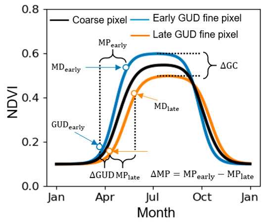
Figure 1. Illustration of three factors ($\Delta GU{D}_{\mathrm{fine}},\Delta M{P}_{\mathrm{fine}},\Delta G{C}_{\mathrm{fine}}$) for a composite case in which the coarse pixel contains two fine pixels. Two fine pixels were represented as the double-logistic curves to illustrate the whole vegetation index (VI) time-series of vegetation. MD refers to the maturity date.

The meanings of the parameters GUD, MP and GC are easy to understand. The MP and GC represent the growth speed of VI, defined as the amount of increasing in VI per unit time, at the horizontal axis (time required) and vertical axis (the range of VI). Therefore, the Bias in the left of Equation (1) can be represented as a function of GUD, MP and GC, and Equation (6) can be rewritten as:

$$Bias=f\left(GU{D}_{\mathrm{fine},1},M{P}_{\mathrm{fine},1},G{C}_{\mathrm{fine},1},GU{D}_{\mathrm{fine},2},M{P}_{\mathrm{fine},2},G{C}_{\mathrm{fine},2}\right)$$

(8)

Previous studies have suggested that the scale effect is mainly caused by the difference among fine pixels within a coarse pixel [5,6,18]. Based on Equation (8), we therefore assume that the bias is mainly influenced by the difference in the parameters between two fine pixels (i.e., $\Delta GU{D}_{\mathrm{fine}}$, $\Delta M{P}_{\mathrm{fine}}$, and $\Delta G{C}_{\mathrm{fine}}$). Thus, Equation (8) becomes:

$$Bias=f\left(\Delta GU{D}_{fine},\Delta M{P}_{fine},\Delta G{C}_{fine}\right)$$

(9)

The three factors ($\Delta GU{D}_{\mathrm{fine}}$, $\Delta M{P}_{\mathrm{fine}}$ and $\Delta G{C}_{\mathrm{fine}}$) are considered as the biophysical factors that influence the GUD at coarse pixels, which is illustrated in Figure 1.

2.4. Form of Function f in Equation (9)

We divided the function f in Equation (9) into two parts: (1) the bias caused only by $\Delta GU{D}_{\mathrm{fine}}$, and (2) the bias caused by heterogeneity of growth speed at a given $\Delta GU{D}_{\mathrm{fine}}$, expressed as:

$$Bias=bia{s}_{\Delta GU{D}_{\mathrm{fine}}}+bia{s}_{\Delta M{P}_{\mathrm{fine}},\Delta G{C}_{\mathrm{fine}}|\Delta GU{D}_{\mathrm{fine}}}$$

(10)

For simplicity, we assume that the effects of $\Delta M{P}_{\mathrm{fine}}$ and $\Delta G{C}_{\mathrm{fine}}$ on $Bias$ are independent of each other, so Equation (10) can be rewritten as:

$$Bias=bia{s}_{\Delta GU{D}_{\mathrm{fine}}}+bia{s}_{\Delta M{P}_{\mathrm{fine}}|\Delta GU{D}_{\mathrm{fine}}}+bia{s}_{\Delta G{C}_{\mathrm{fine}}|\Delta GU{D}_{\mathrm{fine}}}$$

(11)

To be strict, the effects of $\Delta M{P}_{\mathrm{fine}}$ and $\Delta G{C}_{\mathrm{fine}}$ may not be independent and thus there may be interactions between $\Delta M{P}_{\mathrm{fine}}$ and $\Delta G{C}_{\mathrm{fine}}$ at a certain $\Delta GU{D}_{\mathrm{fine}}$. However, incorporating the interaction effect could make the scale-effect model more complicated and difficult to parameterize. We thus employed the three main items in Equation (11) and investigated the performance of the model in explaining the scale effect.

We explored the possible function forms of each item in Equation (11) by conducting simulation experiments for three scenarios. In scenario I, we simulated two VI curves for the fine pixel 1 and pixel 2 with different GUD but identical MP and GC. We assumed that GUD for pixel 1 was fixed DOY 110, whereas the GUD of pixel 2 varied between DOY 90 and 130 (the GUD difference changes from −20 to 20 days), which was used to analyze variation in $\Delta GU{D}_{\mathrm{fine}}$ (Figure 2a). This scenario shows that $bia{s}_{\Delta GU{D}_{\mathrm{fine}}}$ values varies with $\Delta GU{D}_{\mathrm{fine}}$ in a quadratic function (Figure 2d):

$$bia{s}_{\Delta GU{D}_{\mathrm{fine}}}=c_1\Delta GU{D}_{\mathrm{fine}}^2$$

(12)

where $c_1$ is the fitting parameter. Negative bias in Figure 2d suggests an advanced $GU{D}_{\mathrm{coarse}}$ caused by the scale effect, indicating that $\Delta GU{D}_{\mathrm{fine}}$ between fine pixels will lead to an earlier $GU{D}_{\mathrm{coarse}}$.

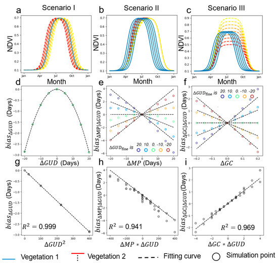
Figure 2. Results of the simulation experiments (three scenarios) exploring the function forms of three variables in Equation (11). (a–c) VI Curves 1 (blue) and 2 (red to yellow) in Scenarios I, II, and III. (d–f) $bia{s}_{\Delta GU{D}_{\mathrm{fine}}}$, $bia{s}_{\Delta M{P}_{\mathrm{fine}}|\Delta GU{D}_{\mathrm{fine}}}$, and $bia{s}_{\Delta G{C}_{\mathrm{fine}}|\Delta GU{D}_{\mathrm{fine}}}$ change with the corresponding factors. The negative values of $\Delta M{P}_{\mathrm{fine}}$ and positive $\Delta G{C}_{\mathrm{fine}}$ indicate faster growth speed of pixel 1 than that of pixel 2. The different color of point refers to different levels of $\Delta GU{D}_{\mathrm{fine}}$ (i.e., −20, −10, 0,10 and 20 days) and the negative $\Delta GU{D}_{\mathrm{fine}}$ values indicate earlier green-up date (GUD) of pixel 1 than that of pixel 2. The dashed lines represent the proposed function forms (Equations (12) and (13)) used to fit these bias values. (g–i) Fitting performance of each function form, respectively.

In scenario II, we investigated the effect of $\Delta M{P}_{\mathrm{fine}}$ on bias ($bia{s}_{\Delta M{P}_{\mathrm{fine}}|\Delta GU{D}_{\mathrm{fine}}}$) at different levels of $\Delta GU{D}_{\mathrm{fine}}$ (Figure 2b). The MP in pixel 1 was fixed at 75 days, whereas that of pixel 2 changed from 55 to 95 days to simulate different $\Delta M{P}_{\mathrm{fine}}$ values (−20 to 20 days). In addition, we set the GUD of pixel 1 from DOY 90 to 130 and fixed the GUD in pixel 2 at DOY 110 to simulate different levels of $\Delta GU{D}_{\mathrm{fine}}$ (−20, −10, 0, 10, 20 days). As shown in Figure 2e, at a given level of $\Delta GU{D}_{\mathrm{fine}}$, the bias caused by $\Delta M{P}_{\mathrm{fine}}$ approximately follows a linear function. In addition, a greater effect of $\Delta M{P}_{\mathrm{fine}}$ on bias is observed when $\Delta GU{D}_{\mathrm{fine}}$ is larger (Figure 2h). Scenario III (Figure 2c) was the same scenario II but for $\Delta G{C}_{\mathrm{fine}}$. Similarly, we obtained linear functions between the bias and $\Delta G{C}_{\mathrm{fine}}$ (Figure 2f). Based on these observations, we used the following equations to describe their effect in scenarios II and II:

$$bia{s}_{\Delta M{P}_{\mathrm{fine}}|\Delta GU{D}_{\mathrm{fine}}}=c_2\Delta GU{D}_{\mathrm{fine}}\times \Delta M{P}_{\mathrm{fine}}$$

$$bia{s}_{\Delta G{C}_{\mathrm{fine}}|\Delta GU{D}_{\mathrm{fine}}}=c_3\Delta GU{D}_{\mathrm{fine}}\times \Delta G{C}_{\mathrm{fine}}$$

(13)

where $c_2$ and $c_3$ are the fitting parameters.

The linear fitting using Equation (13) achieved $R^2$ values of 0.941 and 0.969 for these variables (Figure 2h,i); the former ($\Delta GU{D}_{\mathrm{fine}}\times \Delta M{P}_{\mathrm{fine}}$) showed a negative slope and the latter ($\Delta GU{D}_{\mathrm{fine}}\times \Delta G{C}_{\mathrm{fine}}$) had a positive slope. Note that a smaller MP and a greater GC both indicate a greater growth speed. The form of Equation (13) suggests that the synchronous change of GUD and growth speed (i.e., positive sign of $\Delta GU{D}_{\mathrm{fine}}\times \Delta G{C}_{\mathrm{fine}}$) can delay $GU{D}_{\mathrm{coarse}}$ and vice versa.

In summary, given that the GUD is derived from the VI curve in the logistic-form, results of the simulation experiments suggest that heterogeneity of $\Delta GU{D}_{\mathrm{fine}}$ leads to an earlier $GU{D}_{\mathrm{coarse}}$, and this advance in $GU{D}_{\mathrm{coarse}}$ is further adjusted by the relationship between $\Delta GU{D}_{\mathrm{fine}}$ and $\Delta M{P}_{\mathrm{fine}}$ or $\Delta G{C}_{\mathrm{fine}}$, which can enhance or offset the negative bias in $GU{D}_{\mathrm{coarse}}$ depending on the reversal and synchronous changes between the GUD and growth speed. Further, it can be deduced that the detected GUD of a coarse pixel is closer to the fine pixel with an earlier GUD and a faster growth speed (shorter MP and greater GC).

By combining Equations (11)–(13), we achieved the final model for estimating the scale effect of GUD for the two-endmember case:

$$Bias=c_1\Delta GU{D}_{\mathrm{fine}}^2+c_2\Delta GU{D}_{\mathrm{fine}}\times \Delta M{P}_{\mathrm{fine}}+c_3\Delta GU{D}_{\mathrm{fine}}\times \Delta G{C}_{\mathrm{fine}}$$

(14)

Following the function form, we generalized Equation (14) for the multi-endmember case by using variance and covariance (i.e., $va{r}_{GUD}$, $co{v}_{MP,GUD}$, and $co{v}_{GC,GUD}$ instead of $\Delta GU{D}_{\mathrm{fine}}^2$, $\Delta GU{D}_{\mathrm{fine}}\times \Delta M{P}_{\mathrm{fine}}$, and $\Delta GU{D}_{\mathrm{fine}}\times \Delta G{C}_{\mathrm{fine}}$, respectively):

$$Bias=c_{1}va{r}_{GU{D}_{\mathrm{fine}}}+c_{2}co{v}_{M{P}_{\mathrm{fine}},GU{D}_{\mathrm{fine}}}+c_{3}co{v}_{G{C}_{\mathrm{fine}},GU{D}_{\mathrm{fine}}}$$

(15)

Next, we describe a series of experiments designed to test Equations (14) and (15).

3. Experimental Design

3.1. Simulation Experiments Based on PhenoCam Sites Data

3.1.1. Phenology Observations

We collected some typical vegetation greenness annual curves from eight phenological camera observation sites (Table 1) provided by the PhenoCam website [19] (https://phenocam.sr.unh.edu/webcam/). PhenoCam data were used because digital photographs at the ground were cloud-free and were taken repeatedly at a high temporal frequency (e.g., 0.5 h). We calculated the green chromatic coordinate (GCC) and used it as the indicator of land-surface greenness, according to previous studies [20,21,22]:

$$GCC=\frac{G}{R+G+B}$$

(16)

where R, G, and B represent digital numbers at the red, green, and blue bands, respectively. We generated the time-series of GCC to represent the annual greenness change of vegetation at each site (Figure 3).

Table 1. Details of the eight sites where data were gathered for GCC curves used for the simulation. The abbreviations of vegetation types are switchgrass (SG), miscanthus (MC), grassland (GR), deciduous needleleaf (DN), deciduous broadleaf (DB), mixed vegetation (MX), shrubs (SH), and tundra (TN).

Site ID	Site Name	Type	Year	Longitude	Latitude	GUD	MP	GC
WG	uiefswitchgrass	SG	2014	−88.197	40.064	118.2	28.0	0.073
MC	uiefmiscanthus	MC	2012	−88.198	40.063	116.2	28.2	0.082
UP	uiefprairie	GR	2011	−88.197	40.064	98.1	45	0.112
TG	torgnon-ld	DN	2013	7.561	45.824	156.0	16.9	0.087
BV	bitterootvalley	DB	2014	−114.091	46.507	110.3	51.8	0.065
CO	canadaOBS	MX	2012	−105.118	53.987	86.4	88.1	0.054
CC	contactcreek	SH	2012	−155.923	58.208	154.6	32.7	0.033
CV	coville	TN	2011	−155.563	58.803	141.7	92.3	0.030

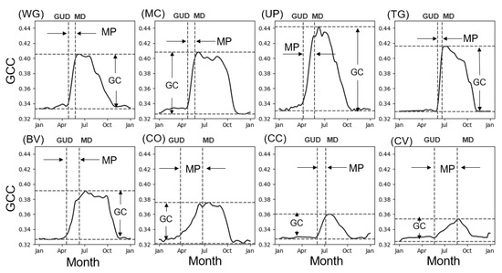
Figure 3. Green chromatic coordinate (GCC) curves of eight vegetation sites derived from PhenoCam data. The vegetation type at each site (identification (ID) in parentheses) is listed in Table 1.

3.1.2. Testing the Two-Endmember Model

We used the PhenoCam data to test the two-endmember model in Equation (14). For this, we repeatedly chose two curves from the eight GCC curves (Figure 3) at each time, which generated a total of 28 combinations. In each combination, we first mixed the two curves ($GC{C}_{\mathrm{fine}}$) with equal proportions to simulate the GCC curve of a coarse pixel ($GC{C}_{\mathrm{coarse}}$) according to Equation (4). We then calculated $\Delta GU{D}_{\mathrm{fine}}$, $\Delta M{P}_{\mathrm{fine}}$, and $\Delta G{C}_{\mathrm{fine}}$ between the two $GC{C}_{\mathrm{fine}}$ curves. The bias, as an indicator of the scale effect (Equation (3)), was calculated as the difference between the GUD of $GC{C}_{\mathrm{coarse}}$ and the average of GUD of the two $GC{C}_{\mathrm{fine}}$ curves. The model includes three influential factors ($\Delta GU{D}_{\mathrm{fine}}$, $\Delta M{P}_{\mathrm{fine}}$, and $\Delta G{C}_{\mathrm{fine}}$), so for comparison, we also performed linear fitting at each time by only employing one factor. Finally, the bias values in all 28 combinations were fitted by the proposed two-endmember model and the one factor linear model, respectively. Because different equations may have different numbers of parameters, we calculated the adjusted R² and root-mean-square error (RMSE) for evaluations.

3.1.3. Testing the Multi-Endmember Model Based on SIMMAP Simulated Data

We tested the multi-endmember model by using the data simulated by the SIMMAP (simulación de mapas) software [23]. The software can generate landscape spatial patterns that contain various categories of different degrees of landscape fragmentation based on the modified random cluster method. The degrees of landscape fragmentation were control by parameter p, which was defined as the initial probability that a pixel was marked. The larger the p parameter, the smaller the number of patches and the more homogeneous the surface (as shown in Figure 4). More detailed descriptions and download links of SIMMAP can be found on the website: http://www2.montes.upm.es/personales/saura/software.html.

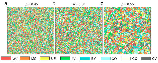
Figure 4. The simulation images from SIMMAP software with different degrees of landscape fragmentation represented by p values of 0.45, 0.50, and 0.55.

We first generated three images (1000 × 1000 pixels) as fine resolution images with different degrees of landscape fragmentation, controlled by the parameter p in SIMMAP (p = 0.45, 0.50, 0.55; Figure 4). In each image, we included the eight vegetation types with equal proportion, and for each type a PhenoCam GCC curve (Table 1) was assigned. We then scaled up the three fine resolution images to coarser with aggregation rates of 3 × 3, 4 × 4, …, 20 × 20 pixels (Figure 5a,b) based on Equation (4). $GU{D}_{\mathrm{coarse}}$, corresponding $GU{D}_{\mathrm{fine}-\mathrm{ave}}$, and three model parameters (i.e., the variance and covariance) were then calculated from coarse and fine resolution images (Figure 5c,d). The bias values were thus calculated as the difference of $GU{D}_{\mathrm{coarse}}$ and $GU{D}_{\mathrm{fine}-\mathrm{ave}}$. Finally, we tested our multi-endmember model on bias at each scale respectively. Note that we randomly split all of the pixels into two-thirds for training (determining the three coefficients in Equation (15)) and one-third for validation.

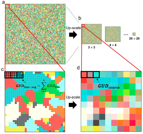
Figure 5. Up-scaling from the fine resolution images to coarser images: (a) fine resolution image, (b) up-scaled coarser images at different scales. (c,d) The example of up-scaling of 3 × 3 pixels and the corresponding calculation of $GU{D}_{\mathrm{fine}-\mathrm{ave}}$ and $GU{D}_{\mathrm{coarse}}$.

3.2. Testing the Multi-Endmember Model Based on Landsat-MODIS Fused EVI2 Data

We further employed the same satellite data used by Zhang et al. [5] to test the multi-endmember model. The $GU{D}_{\mathrm{fine}}$ image (Figure 6) was estimated form Landsat-MODIS fused EVI2 (a two-band EVI [24]) in 2014 with a spatial resolution of 30 m and a frequency of 3 days. The study area was in central Iowa, USA, and mainly includes nine land-cover types: corn, soybean, hay, other crops, grass, forests, shrubs, non-vegetated areas, and open water/wetlands. More detailed information regarding the data was reported by Zhang et al. [5].

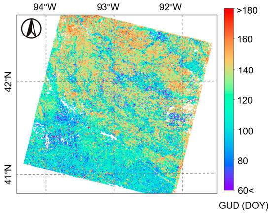
Figure 6. The GUD detected from fine resolution MODIS-Landsat fused EVI2 images.

Likewise, we simulated coarser satellite images by up-scaling the EVI2 data from 30 m to 150, 210, 270, 330, 390, and 450 m, which corresponds to aggregation rates of 5 × 5, 7 × 7, 9 × 9, 11 × 11, 13 × 13, and 15 × 15, respectively. During this process, we excluded some pixels with missing observations or inaccurate phenology estimations, as suggested by Zhang et al. [5]. Up-scaling operations can avoid the errors caused by geometric registration, atmospheric effect, and sensor differences, which allowed us to focus on the scale effect rather than other factors. We again randomly selected two-thirds of the pixels as training data and the remaining pixels were used for validation.

4. Results

4.1. Performance of the Two-Endmember Model

Performance of the two-endmember scale-effect model on 28 mixed GCC curves is shown in Figure 7. It can be seen that the two-endmember model achieved good performance (R²_adj = 0.826, RMSE = 5.53 days), suggesting its ability to account for the scale effect (Figure 7a). Linear models with only one factor performed poorly, with R²_adj < 0.2 and RMSE > 12 days (Figure 7b–d). These investigations emphasized that integrating the three influential factors with a proper function form is very important for explaining the scale effect.

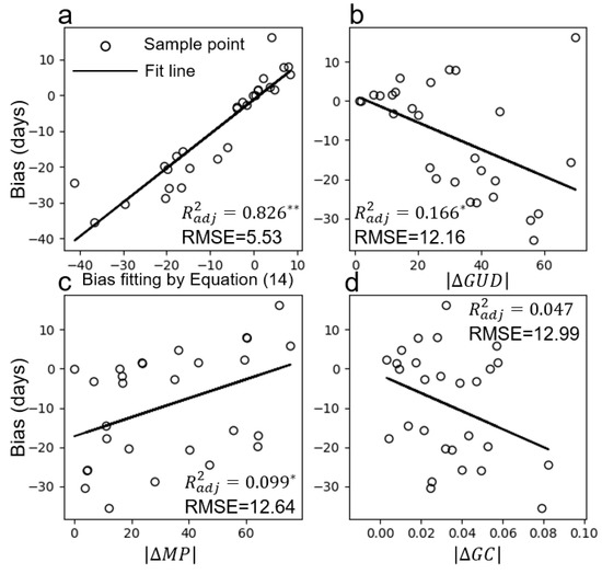
Figure 7. (a) Model fitting using the two-endmember model (Equation (14)) and (b–d) linearly fitting using only one of the three influential factors. Note that the bias is unrelated to the sign of the factor in three linear factor models, so we used the absolute values of the factors in (b–d) to not account for their signs. ** p < 0.01, * p < 0.05.

4.2. Performance of Multi-Endmember Model Based on SIMMAP Simulated Data

We showed the changing patterns of the average of bias ($\overline{\mathrm{bias}}$) values at different scales for the training and validation datasets, respectively (Figure 8a,d). The average of bias (negative values) decreases as scale becoming coarser under all conditions of landscape fragmentation (p = 0.45, 0.50, and 0.55), suggesting a greater scale effect for larger differences of spatial resolution between images. Moreover, we found larger absolute values of $\overline{\mathrm{bias}}$ in the image with higher landscape fragmentation (i.e., lower p values), which suggests that the scale effect is more obvious in heterogeneous areas. We used the proposed multi-endmember model to fit the bias values and achieved $R^2>$ 0.6 for all landscapes, both for training and validation data (Figure 8).

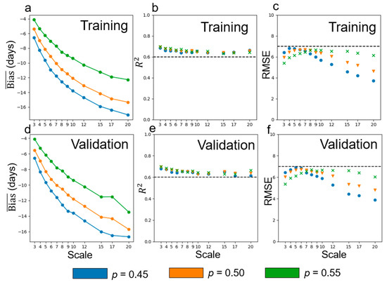
Figure 8. (a,d) The average of bias values change as the training and validation dataset scale (size of the aggregated window) changes; (b–f) Performance of the multi-endmember model at different scales for training and validation datasets in terms of the $R^2$ and root-mean-square error (RMSE, days) values.

4.3. Performance of Multi-Endmember Model Based on MODIS-Landsat Fused EVI2 Data

We presented the average of bias values at various scales of Landsat-MODIS fused EVI2 images in Figure 9a,d. We found a similar decreasing pattern at the larger scale, as that in Figure 8, which confirms a more considerable scale effect when the spatial resolution became coarser. We fitted these bias values by using our multi-endmember model and achieved the performance with $R^2$ > 0.56 and RMSE < 2.3 days. Taking 450-m resolution as an example, we showed the scatter plot (1:1 line) of bias and predicted bias in Figure 10. An $R^2$ > 0.70 in the validation dataset was achieved by the proposed model. Furthermore, in addition to the negative bias values, the model can also account for the positive bias values (Figure 10), suggesting that the new model can explain the delayed $GU{D}_{\mathrm{coarse}}$, which was not well understood in previous studies [6].

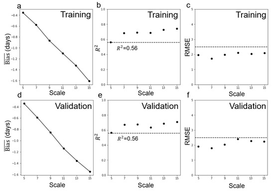
Figure 9. The same as Figure 8, but for the Landsat-MODIS fused EVI2 data. Scale refers to the size of the aggregated window.

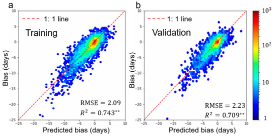
Figure 10. Performance of the multi-endmember model at the scale of 450-m resolution for the (a) training dataset (b) and validation dataset. ** p < 0.01.

5. Discussion

5.1. Conceptual Explanations of the Scale Effect

Previous studies attributed the scale effect of detected GUD to the heterogeneity of land cover or GUD [5,6]. However, in this study, we found that the scale effect is explained by the heterogeneities both of GUD and vegetation growth speed during spring. We further incorporated these factors into the scale-effect model (Equation (15)) that we developed. The good performance of the model in a series of experiments provided the rationale for clarifying these influential factors. Here, we further demonstrated in detail why the scale effect is influenced by these three factors and how they can be used to explain some phenomena of caused by scale effect (i.e., the scale effect increases with up-scaling and $GU{D}_{\mathrm{coarse}}$ maybe later than $GU{D}_{\mathrm{fine}-\mathrm{ave}}$ in some areas).

First, we graphically explain why the detected GUD at a coarse pixel is earlier than the average of GUDs of all fine pixels within it, a phenomenon reported recently [5], and further why this tendency is stronger with greater heterogeneity of GUD. We simulated two coarse pixels (pixels A and B in Figure 11a,b) by the linear spectral mixture model, in which the average GUDs of fine pixels are identical and all the VI curves of corresponding fine pixels have exactly the same shape (no difference in GC and MP) but have differences in GUD and their proportions. The heterogeneity of GUD for pixel B is larger than that for pixel A (bottom-right insets of Figure 11a,b). It can be observed that the VI curve for pixel B with greater GUD heterogeneity obviously increases earlier in spring than pixel A, and thus, pixel B has an earlier GUD (Figure 11c). Such an advance (negative bias) is mainly because the larger number of fine pixels with earlier GUD in pixel B makes a greater contribution to VI values of the mixed coarse pixel in spring, by the linear spectral mixture model. This simulation experiment highlights that the spectral mixture process in VI can linearly propagate the heterogeneity of GUD from the fine scale to the coarse scale, leading to a significant scale effect.

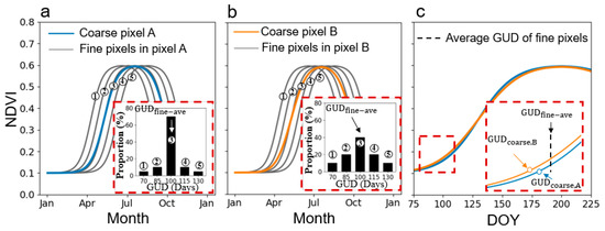
Figure 11. A simulation experiment is designed to help understand the influence of heterogeneity of GUD on scale effect. (a,b) Coarse pixels A and B consist of five fine VI curves with five different GUD values but the same VI curve shape. However, the shape of the coarse VI curves is different from the shape of fine VI curves. The heterogeneity of GUD is larger in pixel B than that in pixel A, as shown by the histograms of fine pixel GUD in the bottom-right; (c) The VI curves for coarse pixels A and B derived from the linear spectral mixture model, respectively. $GU{D}_{\mathrm{coarse},\mathrm{B}}$ is earlier than $GU{D}_{\mathrm{coarse},\mathrm{A}}$ and they are both earlier than $GU{D}_{\mathrm{fine}-\mathrm{ave}}$ (the vertical dashed line in the right of $GU{D}_{\mathrm{coarse},\mathrm{A}}$).

Next, we demonstrated why heterogeneity of MP and GC under the condition of GUD heterogeneity can also influence the scale effect. We simulated three coarse pixels (pixels A, B, and C; black lines in Figure 12a, Figure 12b and Figure 12c, respectively) consisting of two fine pixels with different GUDs (blue and orange curves). The three coarse pixels have identical GUDs of corresponding fine pixels, but the later green-up fine pixel (orange line) in pixels B and C has smaller MP or greater GC. It is clear that the fine pixels with smaller MP or greater GC have greater amplitude of $K^{\prime }$ (orange lines in Figure 12e,f). Consequently, the fine pixel with greater $K^{\prime }$ values caused by greater growth speed (smaller MP or greater GC) contributes more in the $K^{\prime }$ mixing process, making the GUD of pixel B or C later than that of pixel A and closer to that of the later fine pixel with faster growth speed and greater $K^{\prime }$ value (Figure 12b,d). Combining Figure 11 and Figure 12, it is clear that the heterogeneity of GUD, MP, and GC leads to scale effect from the fine to coarse scales through the linear mixture process both in VI and $K^{\prime }$, meaning that the larger the heterogeneity of the three factors, the more significant the scale effect.

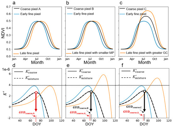
Figure 12. A simulation experiment is designed to help understand the influence of heterogeneity of growth speed on scale effect. (a–c) The coarse VI curves (black curves) mixed by two fine VI curves (blue and yellow curves) with the same $\Delta GU{D}_{\mathrm{fine}}$ but different $\Delta M{P}_{\mathrm{fine}}$ or $\Delta G{C}_{\mathrm{fine}}$ (to represent different growth speeds); (b–d) The corresponding change rate of curvature ($K^{\prime }$) of these VI curves. The $K^{\prime }$ of coarse curves (black solid lines) is approximated by linear mixing of two $K^{\prime }$ values of fine curves (black dashed lines).

Our findings are based on the GUD detected by the curvature method. Here, we further used the widely-used relative threshold method (10% and 20% relative threshold) to estimate GUD and investigated whether the scale effect can still be accounted for by the three proposed factors (i.e., $\Delta GUD$, $\Delta MP$, and $\Delta GC$). We performed the same experiments as those in Figure 2, and found that the relationship between the GUD bias and the three factors (Figure 13) was similar to those based on the curvature method (Figure 2d–f). Nevertheless, we observed that the range of the change in the bias with respect to those three factors based on the relative threshold method seems to be slightly smaller than that based on the curvature method. For example, when $\Delta GUD$ varies between −20 and 20 days, the change of the bias values caused by $\Delta GUD$ are 3 and 2.5 days for the curvature method and the relative threshold method, respectively (comparing Figure 2d–f with Figure 13). These small differences are probably because the relative threshold method is slightly less sensitive to scale effects, compared with the curvature method [11]. The scale effects on GUD estimated using the relative threshold method can also be explained by the three factors proposed in this study.

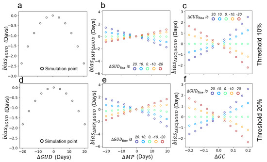
Figure 13. The same as Figure 2d–f, but using the relative threshold method. (a–c) $bia{s}_{\Delta GU{D}_{\mathrm{fine}}}$, $bia{s}_{\Delta M{P}_{\mathrm{fine}}|\Delta GU{D}_{\mathrm{fine}}}$, and $bia{s}_{\Delta G{C}_{\mathrm{fine}}|\Delta GU{D}_{\mathrm{fine}}}$ change with the corresponding factors with 10% relative threshold. (d–f) The same as Figure 13a–c, but using different relative threshold (20%). For comparison, the range of Y-axis is consistent with that in Figure 2d–f.

We conducted an up-scaling experiment over the contiguous United States. Our results confirmed the findings in Peng et al. [6] and also found that $GU{D}_{\mathrm{coarse}}$ occurred later in the processing of up-scaling in some area, which indicates a positive bias (later green-up for coarse pixel; Figure 7 and Figure 10). The influence of growth speed of the fine-pixel VI curve may explain these observations. As we discussed earlier, the scale effect is caused by two kinds of biases (Equation (10)), which are accounted for by the heterogeneity of GUD and that of growth speed, respectively. The bias due to GUD heterogeneity is systematically negative (earlier green-up for coarse pixel), but the sign of the second bias depends on whether the change of GUD and growth speed is synchronous. In other words, when the growth speed of vegetation with later GUD is significantly greater than that with early GUD, the heterogeneity of growth speed will lead to a positive bias and even exceed the advanced effect caused by the negative former bias, eventually resulting in a positive bias. Therefore, our study highlights the importance to consider the heterogeneity of the growth speed of vegetation in the GUD up-scaling method, rather than to only consider the heterogeneity of GUD. For example, the spatial variability in the threshold of percentile method [5], observed by Peng et al. [7], may be caused by ignoring the heterogeneity of growth speed.

5.2. Implications and Limitations

Understanding the scale effect of the VI on GUD detection is useful for cross-scale comparisons and validation of satellite VI-derived phenology. Considering the coarse spatial resolution of commonly used VI products, which ranges from 250 m to 8 km, heterogeneity inevitably exists for most of the Earth’s land surface and consequently leads to significant discrepancy among cross-scale comparisons and validations [5,25].

Our analyses suggest that it is helpful to reduce uncertainty to perform cross-scale phenology validation or evaluation of remote-sensing retrieval of phenology based on observations of a homogenous land surface in terms of the influential factors (i.e., the heterogeneity of GUD, MP, GC). For a heterogeneous surface, a practical solution is to include the scale effect in the process of comparison or validation. Table 2 lists a set of coefficients of the proposed scale-effect model for both simulation data (taking p = 0.5 as an example) and Landsat-MODIS fused EVI2 data. The standardized coefficients indicate the different importance of each item, and the unstandardized coefficients values are relatively stable across scales for different surfaces, suggesting the possibility of estimating scale-derived bias, once we have developed the model for different surfaces. Accordingly, the scale-derived bias estimation will provide a reference that excludes the scale effect or will help estimate uncertainty.

Table 2. The model coefficients (${\mathrm{c}}_1$, ${\mathrm{c}}_2$, ${\mathrm{c}}_3$) in simulation data (taking p = 0.5 as an example) and Landsat-MODIS fused EVI2 data. Scale refers to the size of the aggregated window.

Type	Scale	${\mathbf{c}}_1$		${\mathbf{c}}_2$		${\mathbf{c}}_3$
		Standardized	Unstandardized	Standardized	Unstandardized	Standardized	Unstandardized
Simulation data (p = 0.5)	3	−0.76	−0.035	−0.61	−0.031	0.29	14.5
	4	−0.73	−0.035	−0.60	−0.030	0.30	14.6
	5	−0.72	−0.035	−0.60	−0.030	0.31	14.7
	6	−0.72	−0.035	−0.62	−0.029	0.30	15.0
	7	−0.72	−0.036	−0.61	−0.030	0.30	14.8
	8	−0.71	−0.037	−0.60	−0.032	0.32	13.6
	9	−0.73	−0.036	−0.63	−0.030	0.33	14.7
	10	−0.72	−0.035	−0.62	−0.029	0.33	14.9
	12	−0.75	−0.036	−0.65	−0.029	0.31	15.0
	15	−0.75	−0.036	−0.64	−0.029	0.34	15.2
	17	−0.78	−0.037	−0.64	−0.029	0.33	14.4
	20	−0.90	−0.036	−0.78	−0.029	0.28	14.8
Landsat-MODIS fused data	5	−1.68	−0.037	−1.36	−0.032	0.23	1.61
	7	−1.84	−0.039	−1.45	−0.033	0.27	1.69
	9	−1.72	−0.039	−1.29	−0.033	0.25	1.71
	11	−1.67	−0.038	−1.24	−0.032	0.24	1.58
	13	−1.71	−0.039	−1.25	−0.033	0.25	1.69
	15	−1.70	−0.040	−1.23	−0.034	0.26	1.78

In the temperature-limited biomes (e.g., temperate forests), green-up of a plant species mainly depends on whether the accumulated spring temperature required for green-up is satisfied or not [26,27]. For a heterogeneous surface, the accumulated temperatures required by various species can be quite different [28,29], which may lead to substantial GUD heterogeneity. However, such GUD heterogeneity can vary among years due to temperature fluctuation, even if the vegetation community composition remains unchanged. In years with a warmer spring, the more favorable temperature conditions and faster temperature increase can make it easier to satisfy the requirements of accumulated temperature for different species. Thus, GUD heterogeneity among species may be reduced in these years [30]. Accordingly, it is reasonable to speculate that the heterogeneity of GUD within a coarse pixel could be smaller in years with a warmer spring than in those with a colder spring. Consequently, validation performed in warmer spring years may be less affected by the scale effect. Therefore, we recommend using data in warmer spring years to conduct validation. Moreover, such interannual variations of scale effect caused by different GUD heterogeneity could further contribute to the phenological temporal changes in heterogeneous areas. In particular, the advance of remotely sensed GUD under climatic warming in recent decades [31] could have been partly underestimated, because the negative bias of GUD caused by its heterogeneity in warmer years is smaller than the colder years. This point should be addressed when analyzing the response of phenology metrics to climate change for ecosystems detected by coarse VI products.

We recognize that our current scale-effect analyses still have some limitations. First, our analyses used the logistic function to describe vegetation growth. However, VI time-series data may deviate much from curve of logistic function in some cases (e.g., Figure 3) due to the constraints of various environmental conditions on vegetation growth [32]. Fortunately, the performance of our model in these cases seems to be acceptable (Figure 7 and Figure 8). Further evaluations for scale effect in the case with non-logistic VI curve are necessary in future studies. Second, our investigations were based on up-scaled data rather than on coarse and fine data from different sensors. We did this because various errors from different sensors could not be excluded in the scale-effect analyses, such as differences in imaging conditions, band design and spectral response functions of sensors, and geometric registration, among others. Third, satellite-derived phenology metrics were detected from VI time-series data. Some Vis, such as NDVI, have several known flaws, especially with sensitivity to soil background and spring snowmelt, saturation at moderate to high greenness, and nonlinear scaling [33,34,35]. Clarifying the effects of these complex confounding factors may be needed in future studies to further improve our understanding of the scale effect of land-surface phenology.

6. Conclusions

Our analyses revealed that the scale effect of GUD was controlled by the heterogeneities of both $GU{D}_{\mathrm{fine}}$ and the vegetation growth speed ($M{P}_{\mathrm{fine}}$ and $G{C}_{\mathrm{fine}}$) rather than land-cover or vegetation types. We developed a multivariate scale-effect model (Equation (15)) to account for the GUD bias across different scales. Using both simulated data and MODIS-Landsat fused EVI2 data, we confirmed that the heterogeneity of $GU{D}_{\mathrm{fine}}$ is the most important factor driving the scale effect and this factor directly causes systematically negative bias (i.e., $GU{D}_{\mathrm{coarse}}$ is smaller than $GU{D}_{\mathrm{fine}-\mathrm{ave}}$). The heterogeneity of vegetation growth speed makes the $GU{D}_{\mathrm{coarse}}$ closer to the GUD of vegetation with faster growth, and the direction of the effect (positive or negative bias) depends on whether there is synchronous change in the GUD and growth speed. Our findings provide a mechanistic explanation of the correlation between the scale effect and land-surface heterogeneity, as well as a reference to understand or further convert GUD acquired at different spatial resolutions.

References

- Badeck, F.W.; Bondeau, A.; Bottcher, K.; Doktor, D.; Lucht, W.; Schaber, J.; Sitch, S. Responses of spring phenology to climate change. New Phytol. 2004, 162, 295–309. [Google Scholar] [CrossRef]
- Ganguly, S.; Friedl, M.A.; Tan, B.; Zhang, X.; Verma, M. Land surface phenology from MODIS: Characterization of the Collection 5 global land cover dynamics product. Remote Sens. Environ. 2010, 114, 1805–1816. [Google Scholar] [CrossRef]
- Zhang, X.; Liu, L.; Dong, Y. Comparisons of Global Land Surface Seasonality and Phenology Derived from AVHRR, MODIS and VIIRS Data: Phenology from AVHRR, MODIS and VIIRS. J. Geophys. Res. Biogeosci. 2017, 122, 1506–1525. [Google Scholar] [CrossRef]
- Shen, M.; Zhang, G.; Nan, C.; Wang, S.; Kong, W.; Piao, S. Increasing altitudinal gradient of spring vegetation phenology during the last decade on the Qinghai–Tibetan Plateau. Agric. For. Meteorol. 2014, 89–190, 71–80. [Google Scholar] [CrossRef]
- Zhang, X.; Wang, J.; Gao, F.; Liu, Y.; Schaaf, C.; Friedl, M.; Yu, Y.; Jayavelu, S.; Gray, J.; Liu, L. Exploration of scaling effects on coarse resolution land surface phenology. Remote Sens. Environ. 2017, 190, 318–330. [Google Scholar] [CrossRef]
- Peng, D.; Zhang, X.; Zhang, B.; Liu, L.; Liu, X.; Huete, A.R.; Huang, W.; Wang, S.; Luo, S.; Zhang, X.; et al. Scaling effects on spring phenology detections from MODIS data at multiple spatial resolutions over the contiguous United States. ISPRS J. Photogramm. Remote Sens. 2017, 132, 185–198. [Google Scholar] [CrossRef]
- Peng, D.; Chaoyang, W.; Xiaoyang, Z.; Yu, L.; Huete, A.R.; Wang, F.; Luo, S.; Liu, X.; Zhang, H. Scaling up spring phenology derived from remote sensing images. Agric. For. Meteorol. 2018, 256–257, 207–219. [Google Scholar] [CrossRef]
- Duchemin, B.T.; Goubier, J.; Courrier, G. Monitoring phenological key stages and cycle duration of temporate deciduous forest ecosystems with NOAA/AVHRR data. Remote Sens. Environ. 1999, 67, 68–82. [Google Scholar] [CrossRef]
- Schwartz, M.; Reed, B. Surface phenology and satellite sensor-derived onset of greenness: An initial comparison. Int. J. Remote Sens. 1999, 20, 3451–3457. [Google Scholar] [CrossRef]
- Wang, H.; Liu, D.; Lin, H.; Montenegro, A.; Zhu, X. NDVI and vegetation phenology dynamics under the influence of sunshine duration on the Tibetan plateau. Int. J. Climatol. 2015, 35, 687–698. [Google Scholar] [CrossRef]
- Chen, X.; Wang, D.; Chen, J.; Wang, C.; Shen, M. The mixed pixel effect in land surface phenology: A simulation study. Remote Sens. Environ. 2018, 211, 338–344. [Google Scholar] [CrossRef]
- Fisher, J.I.; Mustard, J.F. Cross-scalar satellite phenology from ground, Landsat, and MODIS data. Remote Sens. Environ. 2007, 109, 261–273. [Google Scholar] [CrossRef]
- Zhang, X.; Friedl, M.A.; Schaaf, C.B.; Strahler, A.H.; Hodges, J.C.F.; Gao, F.; Reed, B.C.; Huete, A. Monitoring vegetation phenology using MODIS. Remote Sens. Environ. 2003, 84, 471–475. [Google Scholar] [CrossRef]
- Friedl, M.A.; Davis, F.W.; Michaelsen, J.; Moritz, M.A. Scaling and uncertainty in the relationship between the NDVI and land surface biophysical variables: An analysis using a scene simulation model and data from FIFE. Remote Sens. Environ. 1995, 54, 233–246. [Google Scholar] [CrossRef]
- Aman, A.; Randriamanantena, H.P.; Podaire, A.; Frouin, R. Upscale integration of normalized difference vegetation index: The problem of spatial heterogeneity. IEEE Trans. Geosci. Remote Sens. 1992, 30, 326–338. [Google Scholar] [CrossRef]
- Kerdiles, H.; Grondona, M.O. NOAA-AVHRR NDVI decomposition and subpixel classification using linear mixing in the Argentinean Pampa. Int. J. Remote Sens. 1995, 16, 1303–1325. [Google Scholar] [CrossRef]
- Shang, R.; Liu, R.; Xu, M.; Liu, Y.; Zuo, L.; Ge, Q. xThe relationship between threshold-based and inflexion-based approaches for extraction of land surface phenology. Remote Sens. Environ. 2017, 199, 167–170. [Google Scholar] [CrossRef]
- Doktor, D.; Bondeau, A.; Koslowski, D.; Badeck, F.W. Influence of heterogeneous landscapes on computed green-up dates based on daily AVHRR NDVI observations. Remote Sens. Environ. 2009, 113, 2618–2632. [Google Scholar] [CrossRef]
- Richardson, A.D.; Hufkens, K.; Milliman, T.; Aubrecht, D.M.; Chen, M.; Gray, J.M.; Johnston, M.R.; Keenan, T.F.; Klosterman, S.T.; Kosmala, M. Tracking vegetation phenology across diverse North American biomes using PhenoCam imagery. Sci. Data 2018, 5, 180028. [Google Scholar] [CrossRef]
- Soudani, K.; Maire, G.L.; Dufrêne, E.; François, C.; Delpierre, N.; Ulrich, E.; Cecchini, S. Evaluation of the onset of green-up in temperate deciduous broadleaf forests derived from Moderate Resolution Imaging Spectroradiometer (MODIS) data. Remote Sens. Environ. 2008, 112, 2643–2655. [Google Scholar] [CrossRef]
- Keenan, T.F.; Darby, B.; Felts, E.; Sonnentag, O.; Friedl, M.A.; Hufkens, K.; O’Keef, J.; Klosterman, S.; Munger, J.W.; Toome, M.; et al. Tracking forest phenology and seasonal physiology using digital repeat photography: A critical assessment. Ecol. Appl. A Publ. Ecol. Soc. Am. 2016, 24, 1478–1489. [Google Scholar] [CrossRef]
- Wang, C.; Chen, J.; Wu, J.; Tang, Y.; Shi, P.; Black, T.A.; Zhu, K. A snow-free vegetation index for improved monitoring of vegetation spring green-up date in deciduous ecosystems. Remote Sens. Environ. 2017, 196, 1–12. [Google Scholar] [CrossRef]
- Saura, S.; Martínez-Millán, J. Landscape patterns simulation with a modified random clusters method. Landsc. Ecol. 2000, 15, 661–678. [Google Scholar] [CrossRef]
- Jiang, Z.; Huete, A.R.; Didan, K.; Miura, T. Development of a two-band enhanced vegetation index without a blue band. Remote Sens. Environ. 2008, 112, 3833–3845. [Google Scholar] [CrossRef]
- Liang, L.A.; Schwartz, M.D.; Fei, S.L. Validating satellite phenology through intensive ground observation and landscape scaling in a mixed seasonal forest. Remote Sens. Environ. 2011, 115, 143–157. [Google Scholar] [CrossRef]
- Chuine, I.; Morin, X.; Bugmann, H. Warming, Photoperiods, and Tree Phenology. Science 2010, 329, 277–278. [Google Scholar] [CrossRef] [PubMed]
- Cao, R.; Shen, M.; Zhou, J.; Chen, J. Modeling vegetation green-up dates across the Tibetan Plateau by including both seasonal and daily temperature and precipitation. Agric. For. Meteorol. 2018, 249, 176–186. [Google Scholar] [CrossRef]
- Cong, N.; Shen, M.; Piao, S.; Chen, X.; An, S.; Yang, W.; Fu, Y.H.; Meng, F.; Wang, T. Little change in heat requirement for vegetation green-up on the Tibetan Plateau over the warming period of 1998–2012. Agric. For. Meteorol. 2017, 232, 650–658. [Google Scholar] [CrossRef]
- Murray, M.; Cannell, M.; Smith, R. Date of budburst of 15 tree species in Britain following climatic warming. J. Appl. Ecol. 1989, 26, 693–700. [Google Scholar] [CrossRef]
- Wang, C.; Tang, Y.; Chen, J. Plant phenological synchrony increases under rapid within-spring warming. Sci. Rep. 2016, 6, 25460. [Google Scholar] [CrossRef]
- Shen, M.; Cong, N.; Cao, R. Temperature sensitivity as an explanation of the latitudinal pattern of green-up date trend in Northern Hemisphere vegetation during 1982–2008. Int. J. Climatol. 2015, 35, 3707–3712. [Google Scholar] [CrossRef]
- Cao, R.; Chen, J.; Shen, M.; Tang, Y. An improved logistic method for detecting spring vegetation phenology in grasslands from MODIS EVI time-series data. Agric. For. Meteorol. 2015, 200, 9–20. [Google Scholar] [CrossRef]
- Huete, A.R.; Jackson, R.D. Soil and atmosphere influences on the spectra of partial canopies. Remote Sens. Environ. 1988, 25, 89–105. [Google Scholar] [CrossRef]
- Ding, Y.; Zheng, X.; Kai, Z.; Xin, X.; Liu, H. Quantifying the Impact of NDVIsoil Determination Methods and NDVIsoil Variability on the Estimation of Fractional Vegetation Cover in Northeast China. Remote Sens. 2016, 8, 29. [Google Scholar] [CrossRef]
- Cao, R.; Chen, Y.; Shen, M.; Chen, J.; Zhou, J.; Wang, C.; Yang, W. A simple method to improve the quality of NDVI time-series data by integrating spatiotemporal information with the Savitzky-Golay filter. Remote Sens. Environ. 2018, 217, 244–257. [Google Scholar] [CrossRef]
© 2019 by the authors. Licensee MDPI, Basel, Switzerland. This article is an open access article distributed under the terms and conditions of the Creative Commons Attribution (CC BY) license (http://creativecommons.org/licenses/by/4.0/).