Photogrammetric Solution for Analysis of Out-Of-Plane Movements of a Masonry Structure in a Large-Scale Laboratory Experiment

Abstract

This paper proposes a photogrammetric procedure able to determine out-of-plane movements experienced by a masonry structure subjected to a quasi-static cyclic test. The method tracks the movement of circular targets by means of a coarse-to-fine strategy. These targets were captured by means of a photogrammetric network, made up of four cameras optimized following the precepts of a zero-, first-, and second-order design. The centroid of each circular target was accurately detected for each image using the Hough transform, a sub-pixel edge detector based on the partial area effect, and a non-linear square optimization strategy. The three-dimensional (3D) coordinates of these targets were then computed through a photogrammetric bundle adjustment considering a self-calibration model of the camera. To validate the photogrammetric method, measurements were carried out in parallel to an ongoing test on a full-scale two-story unreinforced masonry structure (5.4 × 5.2 × 5.4-m) monitored with more than 200 contact sensors. The results provided by the contact sensors during one of the load phases were compared with those obtained by the proposed approach. According to this accuracy assessment, the method was able to determine the out-of-plane displacement during the quasi-static cyclic test with a sub-pixel accuracy of 0.58.

1. Introduction

Currently, the remote sensing discipline offers several solutions to analyze the deformation suffered by various structures from a contactless perspective. Examples of its applicability range from large civil infrastructures such as dams [1,2,3] or bridges [4,5,6]—even in a dynamic loading scenarios [7,8]—to laboratory specimens [9,10,11,12,13,14,15,16,17]. Within this context, the laser scanning technology is placed as the most used remote sensing approach [1,2,3,5,9,13] as it can directly provide high-density three-dimensional (3D) data in the form of point clouds. Through the use of these sensors, it is possible to evaluate the deformation suffered by a structure by means of different change detection methods, such as the radial basis approach [3,18], the plane-fitting method [9], or the curve-fitting strategy [19]. These approaches exploit data redundancy, providing better accuracy than the single-point measurement [19]. However, the use of these methods requires the acquisition of several point clouds, one for each stage to be evaluated, and, thus, requires the use of registration strategies (with introduce an additional error source) to place them into a common coordinate system [1]. In addition to this, its measurement principle—based on the emission and reception of a laser beam—within the necessity of having a dense point cloud, requires the investment of several minutes to capture the whole scene. This issue restricts the use of this technology to those cases in which the structure is completely static [3,9,13,18,19].

Another potential approach for the analysis of changes and deformation in structures that does not share this restriction is photogrammetry [4,6,7,8,10,11,12,14,15,17,20,21,22]. This approach, in contrast to laser scanning, is relatively low-cost as it is possible to obtain reliable results by means of common digital single-lens reflex (DSLR) cameras [6,15,16,21,22]. In addition to this, its flexibility makes it possible to evaluate the deformation suffered by different engineering solutions, from small scales (e.g., mechanical tests) [16,21,22,23] to large structures [7,14,15,20]. This property of the ability to capture several images per second makes it possible to use this technology in dynamic scenarios (e.g., shaking table tests) [7,14,17,20,24,25,26,27]. Within this discipline, there are three strategies that are commonly applied in order to evaluate the changes that occur during a scenario: (i) digital image correlation method (DIC) [10,11,12,16]; (ii) structure from motion approach using change detection algorithms (i.e., cloud-to-cloud comparison algorithms) [15,28,29,30]; and (iii) point-tracking approaches [14,20,23,25,26,31]. While the first two methods are able to produce full-field displacement maps, high computational time, as well as the necessity of having a good texture pattern (i.e., large variation of grey values), can hinder their application [32]. These limitations can be especially relevant in cases in which a large number of images are expected and the surface of the specimen is not textured as those shown in Esposito et al. [33], Lowes et al. [20], and Lehman et al. [14], among others. In those cases, an artificial texture needs to be applied on the specimen, which generally implies the application of random distributed black dots over a white layer [32]. This dependence does not apply to point tracking since it requires only the placement of several artificial targets along the monitored structure [27]. In addition, guaranteeing reliability and precision for the generation of photogrammetric results requires the design of a photogrammetric network [34], especially where the structure under analysis is large [3].

This paper proposes a photogrammetric methodology, able to evaluate out-of-plane displacements experienced by masonry structures. To validate the proposed photogrammetric method, the data acquired from contact type sensors in an ongoing experiment on an unreinforced masonry structure were compared with the data obtained from photogrammetry. The case study selected for this purpose was a quasi-static cyclic test on full-scale two-story structures, instrumented with 200 contact type sensors. The structure was tested at the Macolab/Stevinlaboratorium of Delft University of Technology within a large experimental program [5,10,22] in support to the risk and safety assessment of residential buildings in the Groningen area (north part of the Netherlands).

The article is organized as follows: after this introduction, Section 2 introduces the materials and methods used; Section 3 explains the experimental results obtained, as well as the validation of the approach; finally, Section 4 summarizes the conclusions arising from the use of the proposed photogrammetric approach in monitoring out-of-plane displacements of masonry walls during seismic events.

2. Materials and Methods

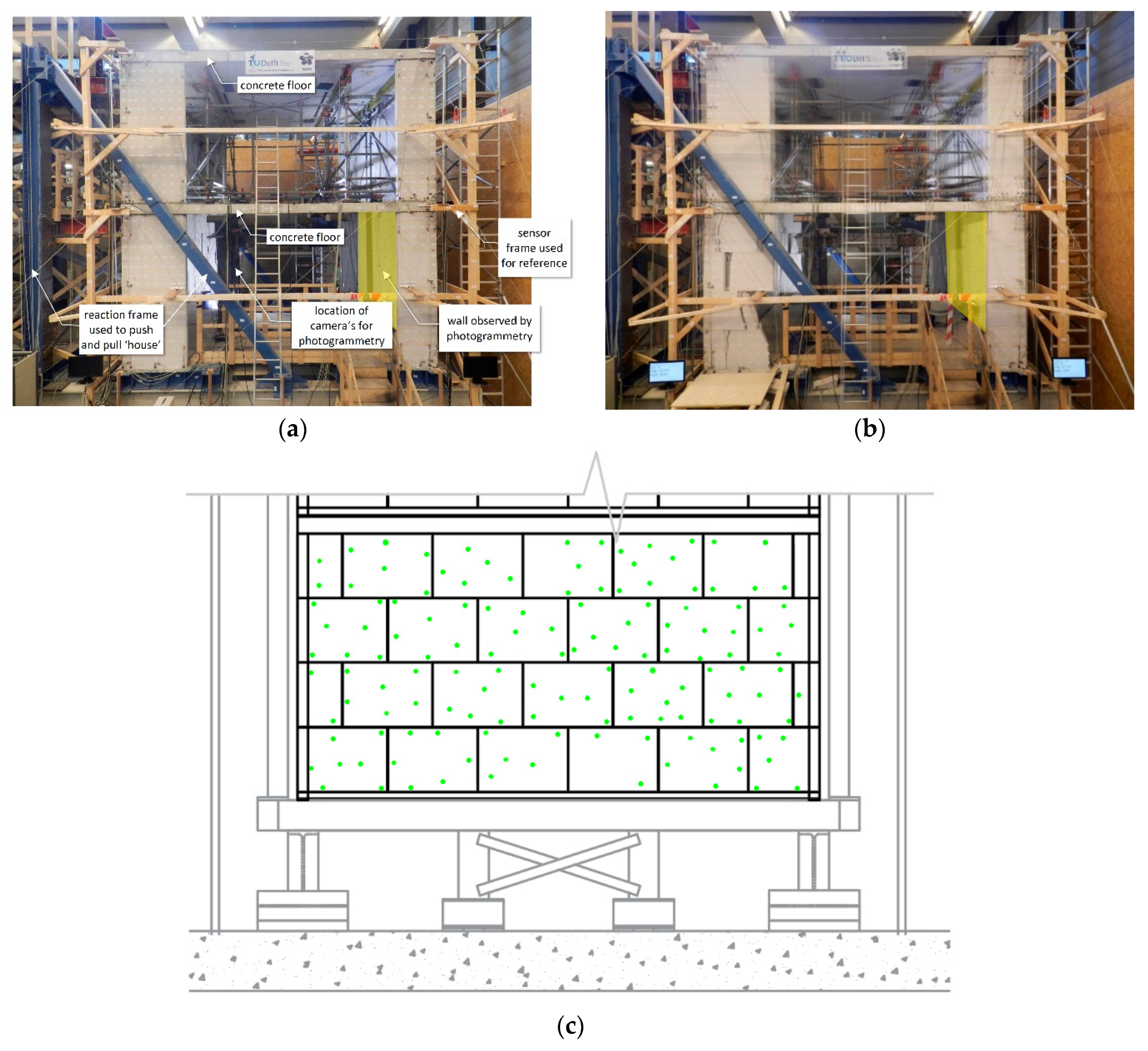
2.1. Quasi-Static Cyclic Test

To validate the photogrammetric method, measurements were carried out in parallel to an ongoing test on a full-scale masonry structure in the Macolab/Stevinlaboratorium of Delft University of Technology. The test aimed at studying the damage evolution in a structure subjected to a horizontal load representative of the seismic loading. For more details on the structural aspects of this experiment, the reader is kindly referred to References [33,35]. The building was a two-story structure having walls made of calcium silicate (CS) element masonry and reinforced concrete slabs as floors (Figure 1). The structure was designed to represent the load-bearing part of a typical Dutch terraced house. It had a floor plan of 5.4 × 5.2 m and a total height of 5.4 m. In top view, the structure can be best seen as two C-shaped walls facing each other. Each C-shaped wall consisted of a transversal wall and two “piers” (pier: term used in structural design for a short wall stabilizing a building against horizontal wind or seismic load) (Figure 1). The piers had two sizes: on the western side (left pier in Figure 1 and Figure 2a), the wide piers PIER1 and PIER3 had a width of 1.1 m, while, on the eastern side (right pier in Figure 1 and Figure 2a), the narrow piers PIER2 and PIER4 had a width of 0.6 m.

The structure was loaded by four actuators, two at each floor level, fixed between the reaction frame and the concrete floors on the west side. A displacement was cyclically imposed (Figure 2) at the second floor level, while a ratio 1:1 was maintained between the forces at the two floor levels. The positive loading direction was defined as displacement from the west to the east side of the structure. More detailed information about the forces applied during the experiment can be found in Reference [33]. Due to the applied displacement, the piers deformed in their own plane, while the transversal walls were subject to out-of-plane deformation. The photogrammetric analysis presented in this paper was performed in the post-peak phase, after reaching the maximum force capacity.

To control the displacements of the actuators and to verify local deformations of the structure, over 200 electronic sensors were placed prior to the tests. The majority of the sensors were displacement measurement devices, such as linear potentiometers and wire potentiometers. These sensors either connected two discrete locations within the structure or they measured its global deformation with respect to an external timber reference frame. These sensors measured with a very high accuracy, in the order of magnitude of a few micrometers. At a number of locations, where physical contact was not possible, the displacements were measured from continuous laser reflections.

2.2. Photogrammetric Approach

A point-tracking photogrammetric method was adopted. This method was chosen since the wall being tested lacked the texture (Figure 2a) to carry out either the photogrammetric approach based on digital image correlation or the structure from motion strategy. To this end, a similar strategy as proposed by Tong et al. [24,25] was used, in which an edge detection algorithm was used to estimate the edges of the targets, followed by a minimization strategy based on the Levenberg–Marquardt method, to estimate the center of the targets. Instead of using a morphological edge detector, our strategy employs state-of-the-art edge detectors based on the partial area effect proposed by Trujillo et al. [36]. This edge detector was used extensively in several recent experimental tests since it provides better accuracies than traditional methods (e.g., the Canny edge detector) [37,38,39]. Additionally, the proposed approach includes the latest advances in camera calibration, based on the self-calibration model [40], as well as the latest strategies for the processing clusters of points such as principal component analysis [41]. This photogrammetric method was used to evaluate the out-of-plane displacements of the east wall at the ground floor (Figure 1). During the test, the east wall experienced limited damage compared with the rest of the structure, mainly consisting of cracking at the top and bottom of the wall [33]. For this reason, it is assumed that a limited error was made while comparing absolute displacement of the wall, measured with contact sensors, with the photogrammetric measurements. The proposed photogrammetric approach is shown in Figure 3.

The proposed photogrammetric approach is shown in Figure 3. Before the data acquisition, a network design was carried out with the aim of optimizing the quality of the photogrammetric network (Section 2.2.2). After the data acquisition, a target detection and matching process was carried out (Section 2.2.3). A network adjustment was performed with the aim of obtaining the external orientation of the camera and the 3D triangulation of the targets. Specifically, this network adjustment followed a threefold approach combining fundamental matrix computation [42], direct linear transformation (DLT) [43], and bundle adjustment [44] (Section 2.2.4). Finally, the movement of each monitored target was tracked by comparing the position of each target with respect to the initial one (Section 2.2.5).

2.2.1. Photographic Sensor

In order to characterize the out-of-plane behavior of the masonry building throughout the quasi-static test, four Basler ace acA2500–14 gm scientific cameras (Basler, Ahrensburg, Germany) equipped with a 4-mm wide-angle prime lens (Basler, Ahrensburg, Germany) were used to perfectly trigger still images. Their technical specifications are illustrated in

Table 1. Technical specifications of the photographic sensors. CMOS—complementary metal–oxide–semiconductor.

Basler acA2500–14 gm
Type of sensor	MT9P031 (CMOS)
Sensor size	5.7 × 4.3 mm
Pixel size	2.2 µm
Resolution (H × V)	2592 × 1944 pixels
Maximum frame rate	14 fps
Focal length	4 mm

. Complementary to this, and with the aim of guarantying the stability of the photogrammetric system during the test, all the cameras were fixed to an isolated steel structure, placed inside the structure, comprising a normal imaging geometry as shown in Figure 1.

Taking into consideration that the point-tracking technique was used in the present study, a total of 138 black circular targets were placed along the entire masonry wall (Figure 1 and Figure 4a). These targets, with a diameter of 35.00 mm, were printed with a high-quality laser printer to ensure a maximum accuracy of the results (Figure 4b).

2.2.2. Photogrammetric Network Design

Prior to the data acquisition, a photogrammetric network was designed with the aim of obtaining accurate and reliable results. Network design involves the spatial distribution of the cameras to monitor the masonry structure based on photogrammetric tasks. Although its definition seems simple, different constraints and design decisions need to be taken. In this case, three different constraints were imposed [45]: (i) to obtain exterior orientation parameters and target coordinates, an optimal datum (i.e., coordinate reference system) was defined (zero-order design, ZOD); (ii) the configuration of an optimal camera geometry, which provided an optimal triangulation of the object coordinates (first-order design, FOD); and (iii) the adoption of suitable measurement precision for the image coordinates, which was reinforced with the coarse-to-fine strategy used for extracting the targets’ centers (second-order design, SOD).

2.2.3. Target Detection and Matching

The reason for choosing circular targets lies in the fact that the distortion of their shape (due to the non-orthogonality between the camera’s sensor and the target) could be expressed mathematically by means of the conic or canonical equation of the ellipse.

Taking this into consideration, the estimation of the ellipse parameters, especially its center, passes through the use of the image coordinates (x and y) of the pixels that belong to the ellipse’s edge. Accordingly, the following coarse-to-fine strategy was implemented. Firstly, the coarse detection of the circular targets was performed based on the Hough transform [46] defining a search window. Secondly, a fine centroid extraction was performed. During this stage, an edge detection algorithm was used, complemented by a non-linear optimization algorithm with the aim of obtaining, with sub-pixel accuracy, the position of the centers of each circular target detected by means of the Hough transform.

An edge detection phase was implemented to define the ellipse that represents each circular target. The edge detector based on the partial area effect proposed by Trujillo-Pino et al. [36] was considered. By extracting image coordinates during the edge detection phase, it is possible to calculate the center of each circular target in each image by a non-linear optimization approach, which finds the optimal conic equation of the ellipse. This non-linear optimization strategy was executed by adopting the Levenberg–Marquardt method [47]. This strategy is highly used in least squares curve-fitting problems due to its robustness [26,48]. In the present study, the considered cost function was as follows:

$$ϵ={\displaystyle \sum }_{i=1}^n{\left(\frac{{\left(x_i-x_0\right)}^2}{a^2}+ \frac{{\left(y_i-y_0\right)}^2}{b^2}-1\right)}^2,$$

(1)

where x_i and y_i are the image coordinates of the detected edge points, x₀ and y₀ are the image coordinates of the centroid of the ellipse, a and b are the length, in pixels, of the main axis of the ellipse, and n denotes the number of pixels matched during the edge detection stage.

2.2.4. Photogrammetric Network Adjustment

The photogrammetric network adjustment consists of the computation of image orientation ($X_{0c}$, $Y_{0c}$, $Z_{oc},$ $r_{i,j}$) together with the triangulation of 3D object points (X,Y,Z). Since the 3D coordinates of the targets are unknown, a first approximation to relative image orientation is provided based on the fundamental matrix (Equation (2)), taking the extracted and matching target centers as input data (Section 2.2.3). The fundamental matrix is independent of scene structure; thus, it can be computed from correspondences of imaged scene points alone, without requiring knowledge of the object coordinates.

$$x^{\prime }x{f}_{11}+x^{\prime }y{f}_{12}+x^{\prime }{f}_{13}+y^{\prime }x{f}_{21}+y^{\prime }y{f}_{22}+y^{\prime }{f}_{23}+x{f}_{31}+y{f}_{32}+f_{33}=0,$$

(2)

where f_ij is the coefficient of the fundamental matrix that encloses the external and internal orientation parameters (without lens distortion), and x, y and x′, y′ are the image coordinates of the extracted and matched target, respectively. At least eight matched targets were required to solve the fundamental matrix and, thus, the relative orientation of images.

Having estimated the relative orientation of images, a direct linear transformation (DLT) was applied to compute the 3D object coordinates of the targets as follows:

$$\left[\begin{array}{ccc}{l}_{4j}-l_{1j}x& l_{5j}-l_{2j}x& l_{6j}-l_{3j}x\\ l_{8j}-l_{1j}y& l_{9j}-l_{2j}y& l_{10j}-l_{3j}y\end{array}\right]\left[\begin{array}{c}X\\ Y\\ Z\end{array}\right]+ \left[\begin{array}{c}{l}_{7j}-x\\ l_{11j}-y\end{array}\right]=V,$$

(3)

where l_i encloses the internal and external orientation of the images linearized by the DLT, x, y represent the image coordinates of the extracted target, X, Y, Z represent the corresponding 3D object coordinates of this target, and V is the residual matrix. Note that the subscript j accounts for the images where the point X, Y, Z appears; therefore, it is required to analyze at least two images (Equation (3)).

Once the external and internal orientation parameters of the camera together with the 3D object coordinates are known, an iterative bundle adjustment, based on collinearity condition, is applied (Equation (4)) in order to refine camera parameters (including lens distortion, $\Delta x^{\prime }$, $\Delta y^{\prime }$ ) and then refine 3D object coordinates.

$$\begin{array}{l}{x}^{\prime }=x_0^{\prime }+f\frac{r_{11}\left(X-X_{oc}\right)+r_{21}\left(Y-Y_{oc}\right)+r_{31}\left(Z-Z_{oc}\right)}{r_{13}\left(X-X_{oc}\right)+r_{23}\left(Y-Y_{oc}\right)+r_{33}\left(Z-Z_{oc}\right)}+ \Delta x^{\prime },\\ y^{\prime }=y_0^{\prime }+f\frac{r_{12}\left(X-X_{oc}\right)+r_{22}\left(Y-Y_{oc}\right)+r_{32}\left(Z-Z_{oc}\right)}{r_{13}\left(X-X_{oc}\right)+r_{23}\left(Y-Y_{oc}\right)+r_{33}\left(Z-Z_{oc}\right)}+ \Delta y^{\prime },\end{array}$$

(4)

where f, $x_o^{\prime }$, $y_o^{\prime }$, $\Delta x^{\prime }$, $\Delta y^{\prime }$ are the inner parameters of the camera, $X_{0c}$, $Y_{0c}$, $Z_{oc},$ $r_{i,j}$ are the external camera parameters, X, Y, Z are the object coordinates, and x’ and y’ are the image coordinates of the targets extracted and matched.

Note that the first part of the bundle adjustment (camera self-calibration) is non-linear; thus, initial approximations and an iterative process are required, whereas the second part (triangulation) is linear and does not require an iterative scheme.

As a result of this photogrammetric approach, a full network defined by the resection of cameras and 3D object coordinates (targets) establishes the reference stage (Figure 3). Last but not least, and in order to compare our results metrically with those provided by sensors (linear potentiometers), the following procedure was applied: (i) estimation of the 3D object coordinates of the target edges with the assistance of the epipolar geometry; and (ii) definition of the model´s scale, confronting the value of the target’s diameters obtained by the photogrammetric approach (expressed in pixels) and their real value (35.00 mm).

2.2.5. Target Tracking and Extraction of Out-Of-Plane Movements

By assuming that the external orientation of each camera remains stable during the experiment, the bundle adjustment obtained during the reference stage was used to estimate the 3D coordinates of each tracked target along the subsequent stages (Figure 3). For this purpose, the following approach was implemented in each set of captured frames:

• Extraction of the new image coordinates of each tracked target: the extraction of the new center coordinates firstly required constraining the search space, i.e., the area within the image in which the target could be found. For the present study case, a search window with a fixed size was used. This value was established in accordance with the size of the targets, the camera resolution, and the expected displacement of the target. Afterward, the coarse-to-fine strategy shown in Section 2.2.3 was applied with the aim of detecting the new target’s centers.
• Estimation of the new 3D coordinates: by assuming that the external orientation of the cameras remained stable along the test, it was possible to use the bundle adjustment solution to estimate the new 3D coordinates. In this sense the collinearity condition (Equation (4)) was applied, using the new image coordinates of the target’s center as input data.

This strategy was repeated in the different sequences (2474 in total). Each set was made up by a total of four images simultaneously acquired by the triggered cameras during the experimental campaign. The 3D coordinates obtained in each stage were later transformed into displacements (difference between the new target’s coordinates and the initial ones).

At this point, it was possible to determine, with sub-pixel accuracy, the center of each monitored target and, thus, the displacements undergone by the masonry wall during the different load steps. However, since the photogrammetric network was solved in a local coordinate system, i.e., the datum of the photogrammetric block was not aligned with the main directions of the masonry wall, an additional step was required. To solve this limitation, an additional step based on the principal component analysis (PCA) approach was carried out. This mathematical strategy can be used to extract the direction of minimum dispersion (first eigenvector) of a dataset (i.e., 3D target’s centers), allowing for the estimation of the normal vector of the masonry wall (Equations (5)–(7)). This consideration allowed establishing a proper photogrammetric datum, being in line with the constraints required for the definition of a ZOD photogrammetric network.

$$\mathsf{\Sigma }={\displaystyle \sum }_{i=1}^k\frac{1}{k}\left(p_i-\overline{p}\right)\ast {\left(p_i-\overline{p}\right)}^T,$$

(5)

where Σ is the covariance matrix, k represents the number of targets tracked, $\overline{p}$ is the centroid made up by all the targets, and $p_i$ the center of target i.

$$\left|\mathsf{\Sigma }- \lambda \ast I=0\right|,$$

(6)

$$\mathsf{\Sigma }\ast v_i={\mathsf{\lambda }}_i\ast v_i,i \in \left\{0,1,2\right\},$$

(7)

where $v_i$ is the column matrix that contains the eigenvector ($v_{i,0}, v_{i,1}, v_{i,2}$) associated with the eigenvalue ${\mathsf{\lambda }}_i$, and I is the identity matrix. Thus, the first eigenvalue (${\lambda }_0)$ corresponds to the direction of minimum dispersion (plane’s normal) whose eigenvector is ($v_{0,0},v_{0,1},v_{0,2}$).

Once the orthogonal direction of the masonry wall was obtained, a six-parameter solid–rigid transformation was achieved over all the target centers tracked. On the one hand, the translation vector was obtained as the difference between the origin of the set of targets and its centroid. On the other hand, the angle between the normal vector of the plane, defined by the coordinates ($v_{0,0},v_{0,1},v_{0,2}$) and the x-axis vector (1,0,0), was used as the rotation vector. Both vectors allowed placing the set of targets in each stage of the test in the proper datum on which the x-axis represents the out-of-plane direction of the wall.

3. Experimental Results

3.1. Network Design and Data Acquisition

The design of the photogrammetric network was established with a set of 138 circular targets distributed all over the masonry wall (Figure 5), and four perfectly triggered still-image cameras located at 3.10 m on the wall (ground sample distance, GSD, of 1.71 mm) in a fixed and stable position, providing a normal imaging geometry (Figure 1, Figure 5 and Figure 6). The photographic acquisition was controlled by a central personal computer (PC) for triggering the four cameras synchronously and storing the images. This resulted in a total of 9896 images with a mean overlap of 61% and a minimum number of three intersecting rays for improving accuracy and reliability. The mean baseline between adjacent images was about 2.21 m, implying a base/depth (B/D) ratio of 0.70. To avoid errors coming from the rolling shutter, the images were acquired under the global reset release shutter mode. Furthermore, velocities of the captured moving object were relatively slow (7 μm/s) compared to the exposure time (order of magnitude of tens of μs). Images were captured with 30-s intervals during several hours of testing.

3.2. Photogrammetric Network Adjustment

The photogrammetric processing was done using a network with only normal images. The datum was arbitrarily defined through the fixed spatial and angular position of cameras and assuming a target diameter of 35.00 mm as a scale factor. The photogrammetric network adjustment was supported by self-developed routines within the mathematical software Matlab R2015b^®.

Specifically, the Hough transformation for circle detection was implemented using as inliers all circles with a radius between 7 and 13 pixels (Figure 7b). To detect the center of the monitored circular targets, the non-linear least squares procedure reported in Section 2.2.3 was applied (Figure 7). During this phase, an average residual was obtained from the circular fitting process of 0.09 pixels (0.15 mm), highlighting the robustness of the process. Within this dataset, a minimum value of 0.05 pixels was obtained in the points placed at the center of the wall, and a maximum value of 0.28 pixels was obtained in the points detected at the edges of the walls. This difference of residuals could be assigned to the geometrical distortion of the lens, which was especially apparent at the edges (Figure 6).

Then, eight centers were manually matched with the homologous center, allowing the introduction of these two-dimensional (2D) coordinates into the workflow defined in Section 2.2.4 and determining the external orientation of the cameras. Finally, the remaining target centers were matched in a semi-automatic way by means of epipolar geometry. These centers were later introduced into the photogrammetry network, allowing the refinement of the external orientation. Between images, the movements of the targets were limited to a small fraction of the absolute size of the targets, so that following the same target from image to image was no problem. It is worth mentioning that, during this adjustment, a self-calibration model based on the Fraser model [49] was implemented with the aim of adapting the inner parameters of each camera to the real conditions of the test (

Table 2. Inner parameters of the camera obtained from laboratory calibration and after the self-calibration.

Parameter		Initial Values (Laboratory Calibration)	Refined Values (Self-Calibration)
Focal length (mm)		4.043 ± 0.002	4.025
Format size (mm)	Height	5.661 ± 0.005	5.655
	Width	4.281 ± 0.005	4.277
Principal point (mm)	X value	2.982 ± 1.314 × 10−3	2.989
	Y value	2.264 ± 2.673 × 10−3	2.233
Radial lens distortion	K1 value	1.502 × 10−2 ± 2.641 × 10−5	1.151 × 10−2
	K2 value	7.084 × 10−5 ± 3.242 × 10−6	4.422 × 10−5
	K3 value	3.447 × 10−6 ± 1.113 × 10−8	3.443 × 10−6
Decentering Lens distortion	P1 value	4.851 × 10−4 ± 1.235 × 10−5	1.334 × 10−4
	P2 value	1.461 × 10−3 ± 3.471 × 10−5	−7.840 × 10−4

). In addition, several invariants (target diameter) were used to scale the photogrammetric model (Figure 8). As a result, it was possible to estimate the spatial position of each camera with a re-projection root-mean-square error (RMSE) error of 0.16 pixels and a relative error in terms of invariants (re-projected diameters) of 1.53% (

Table 3. Accuracy of the photogrammetric model in terms of target diameters (re-projection error). The error in pixels is provided in parentheses. ID—identifier.

ID	Expected Value (mm)	Obtained Value (mm)	Absolute Error (mm)	Relative Error (%)
Chd-1	35.00	34.42	0.58 (0.34)	1.65
Chd-2	35.00	34.96	0.04 (0.00)	0.11
Chd-3	35.00	35.77	−0.77 (0.45)	−2.20
Chd-4	35.00	35.25	−0.25 (0.15)	−0.71
Chd-5	35.00	34.14	0.86 (0.50)	2.45
Chd-6	35.00	35.86	−0.86 (0.50)	−2.45
Chd-7	35.00	34.74	0.26 (0.15)	0.74

). Regarding the checkpoints, the re-projection error obtained had a sub-pixel accuracy of 0.30 pixels (0.52 mm) with a maximum value of 0.50 pixels for those checkpoints placed at positions 3, 5, and 6 (Table 3).

3.3. Analysis of the Out-Of-Plane Displacements Experienced by the Masonry Wall

The subsequent set of images, distributed in 2473 stages, was processed following the approach defined in Section 2.2.5, investing a total of 115 min on an Intel® XEON E3-1240 v3 processor at 3.4 GHz and 16 GB of double data rate 2 (DDR2) random-access memory (RAM) (around 3 s per stage). As a result, it was possible to estimate the displacement undergone by each target during the experiment. As stated in Section 2.2.5, a PCA approach was used to estimate the transformation matrix that allowed transforming the initial photogrammetric datum with respect to the main axis of the wall. A six-parameter solid–rigid transformation was applied over all the targets (

Table 4. Parameters of the three-dimensional (3D) solid–rigid transformation to align the data.

Parameters		Values
Translation	x (mm)	−336.14
	y (mm)	−467.46
	z (mm)	3947.02
Euler angles	φ (°)	−4.67
	θ (°)	−11.54
	Ψ (°)	10.04

). This step was applied in all the sequences (including the reference stage) (Figure 3).

As a consequence, it was possible to evaluate the out-of-plane displacements experienced by the masonry wall during the quasi-static cyclic test in the different cycles (

Table 5. Out-of-plane displacements captured by target 1386.

Cycle	Peak Displacements		Average Velocity (mm/s)	Cycle Duration (s)
	Δ− (mm)	Δ+ (mm)
C17b	−21.38	15.95	0.007	682
C18	−27.46	19.70	0.007	671
C19	−32.72	20.25	0.007	684
C20	−36.68	23.64	0.007	920
C21	−41.48	31.83	0.007	1450
C22	−48.19	44.51	0.007	666

and

Table 6. Out-of-plane displacements captured by target 1134.

Cycle	Peak Displacements		Average Velocity (mm/s)	Cycle Duration (s)
	Δ− (mm)	Δ+ (mm)
C17b	−21.42	16.03	0.007	682
C18	−27.03	20.02	0.007	671
C19	−32.35	20.75	0.007	684
C20	−37.34	24.98	0.007	920
C21	−41.10	33.18	0.007	1450
C22	−48.34	45.93	0.007	666

) (Figure 9). As expected for the considered loading conditions, the target 1464 at mid-height of the wall showed a smaller displacement than the target 1386.

3.4. Accuracy Assessment of the Photogrammetric Approach

With the aim of corroborating the accuracy of the proposed photogrammetric approach, a comparison between the data obtained from the potentiometers and the photogrammetric results was carried out. The comparison was made by considering the displacement measured by the sensors P1 and P2 and the displacement of targets 1134 and 1386, as well as the displacement experienced by targets 1464 and 1199 and the sensors P3 and P4 (Figure 5b). It should be noted that the sensors P1 and P2 were positioned between the reaction frame and the reinforced concrete floor on the west side of the building (Figure 1), whereas the photogrammetric targets refer to the inside surface of the east wall of the building. For the design of the test, it was expected that the floor equally redistributed the imposed load on both the western and eastern walls (Figure 1). To this end, the absolute errors and the root-mean-square error (RMSE) were calculated between the peaks of the different runs carried out (

Table 7. Absolute errors obtained for the comparison between the average values of the peaks captured by target 1386 and sensor P1 after outlier removal. RMSE—root-mean-square error.

Cycle	Average Displacement (Potentiometer)		Average Displacement (Photogrammetry)		Absolute error (Extremes in Bold)		RMSE (mm)
	Δ− (mm)	Δ− (mm)	Δ− (mm)	Δ+ (mm)	Δ− (mm)	Δ+ (mm)
C17b	−21.98	15.80	−21.42	16.03	0.56	0.23	0.94
C18	−27.92	19.18	−27.03	20.02	0.89	0.84
C19	−33.33	19.77	−32.35	20.75	0.98	0.98
C20	−37.46	24.09	−37.34	24.98	0.12	0.89
C21	−42.62	31.68	−41.10	30.40	1.52	−1.28
C22	−47.81	44.32	−48.34	43.94	−0.53	−0.38

,

Table 8. Absolute errors obtained for the comparison between the average values of the peaks captured by target 1134 and sensor P2 after outlier removal.

Cycle	Average Displacement (Potentiometer)		Average Displacement (Photogrammetry)		Absolute Error (Extremes in Bold)		RMSE (mm)
	Δ− (mm)	Δ+ (mm)	Δ− (mm)	Δ+ (mm)	Δ− (mm)	Δ+ (mm)
C17b	−22.02	16.11	−21.31	15.91	0.71	−0.20	1.04
C18	−27.99	19.55	−27.38	19.64	0.61	0.09
C19	−33.52	19.97	−32.63	20.19	0.89	0.22
C20	−37.67	24.19	−36.57	23.57	1.10	−0.62
C21	−42.64	29.46	−41.35	30.48	1.02	−0.37
C22	−47.81	44.87	−48.23	44.06	−0.42	−0.58

,

Table 9. Absolute errors obtained for the comparison between the average values of the peaks captured by target 1199 and sensor P3 after outlier removal.

Cycle	Average Displacement (Potentiometer)		Average Displacement (Photogrammetry)		Absolute Error (Extremes in Bold)		RMSE (mm)
	Δ− (mm)	Δ+ (mm)	Δ− (mm)	Δ+ (mm)	Δ− (mm)	Δ+ (mm)
C17b	−10.10	7.23	−10.10	6.39	0.00	−0.84	1.03
C18	−12.85	9.17	−13.51	7.62	−0.66	−1.55
C19	−15.34	9.19	−15.70	8.26	−0.36	−0.93
C20	−17.34	11.21	−17.62	10.02	−0.28	−1.19
C21	−19.73	13.63	−20.24	12.11	−0.51	−1.52
C22	−21.00	22.69	−19.39	23.11	1.61	−1.58

and

Table 10. Absolute errors obtained for the comparison between the average values of the peaks captured by target 1464 and sensor P4 after outlier removal.

Cycle	Average Displacement (Potentiometer)		Average Displacement (Photogrammetry)		Absolute Error (Extremes in Bold)		RMSE (mm)
	Δ− (mm)	Δ+ (mm)	Δ− (mm)	Δ+ (mm)	Δ− (mm)	Δ+ (mm)
C17b	−10.21	7.07	−10.67	7.46	−0.46	0.39	0.95
C18	−12.94	9.18	−12.86	10.66	0.08	1.48
C19	−15.37	9.01	−15.57	10.15	0.20	1.14
C20	−17.24	11.02	−18.20	11.16	−0.96	0.14
C21	−19.56	13.49	−20.72	15.10	−1.16	1.61
C22	−22.55	20.71	−21.92	21.86	0.63	1.15

). With the aim of neglecting possible outliers, the 3σ cut-off criterion was applied. During this outlier removal stage, a total of 10 measures were not considered: (i) four measures within cycles C21 and C22 for target 1134; (ii) one measure within cycle C22 for target 1386; (iii) three measures within cycles C21 and C22 for target 1199; and (iv) two measures within cycles C21 and C22 for target 1464. As a result of this, the RMSE of the photogrammetric approach was reduced from 1.40 mm (0.82 pixels) to 0.99 mm (0.58 pixels), bearing out the accuracy of the proposed method. It is worth mentioning that this error was similar to the error estimated within the checkpoints (Table 3), suggesting that the photogrammetric platform was stable during the data acquisition.

4. Discussion and Conclusions

This work investigated the use of a contactless method in monitoring the out-of-plane displacements suffered by masonry structures in large-scale laboratory tests, with the aim of overcoming the main limitations of traditional contact sensors. To achieve this, a quasi-static cyclic test on a full-scale two-story unreinforced masonry structure at the Delft University of Technology, in an ongoing experimental campaign, was carried out as a case study. In particular, the out-of-plane deformation of a wall located at the ground floor of the structure was considered in this paper.

The photogrammetric method adopted was based on a target-tracking approach that allowed measuring the displacements suffered by the structure through the use of several circular targets located along its surface. Firstly, the centers of these circular targets were extracted by means of a coarse-to-fine strategy: (i) a coarse detection of each target through the use of the Hough transform; (ii) an extraction, with sub-pixel accuracy, of the target’s edge through an edge extractor based on the partial area effect; and (iii) an accurate extraction of the target’s center by a non-linear least squares optimization procedure that used the data obtained by the edge detector, as well as the canonical equation of the ellipse to determine the optimal position of its center. Secondly, the centers of the tracked targets were used to solve the external orientation of a photogrammetric network, designed under three different constraints (ZOD, FOD, and SOD). This network design, which took into account the base/depth ratio, as well as a proper datum, was used with the aim of optimizing the final accuracy of the photogrammetric approach. Finally, a rigid transformation was defined with the aim of obtaining the normal vector of the wall by principal component analysis, allowing the evaluation of the out-of-plane displacements experienced by the wall during the test.

The results obtained during the present research work highlight the following:

• In comparison with traditional contacted sensors, such as linear variable differential transformers (LVDTs), potentiometers, or displacement gauges, the proposed methodology offers a contactless methodology that is able to monitor the whole surface of the specimen with a unique photogrammetric network and several tracking targets. Complementary to this, the contact nature of the traditional sensors made it necessary to place them in specific positions with the risk of not capturing the deformation suffered by other locations, or even the cracks.
• The residual error obtained during the detection of the circular targets, which was estimated as 0.09 pixels, corroborates the robustness of the proposed approach.
• The proposed method showed great performance, requiring 115 min for processing the whole dataset. This dataset was made up of 9896 images.
• By comparing the measurements obtained via the traditional contact sensors and the contactless method, it was possible to conclude that the photogrammetric approach was able to detect the out-of-plane movements of the masonry wall with sub-pixel accuracy. This accuracy was estimated at 0.58 pixels (0.99 mm).
• The proposed approach can be applied to specimens subjected to quasi-static cyclic tests for which the laser scanning strategy may not be continuously applied due to the time needed to scan each epoch. Highlighting also its low cost, this approach requires the use of several digital cameras and printed targets.
• This method highlights its flexibility through its application in texture-less structures for which the digital image correlation and the structure from motion cannot be applied property. These two methods require the proper preparation of the surface specimen. This preparation involves the application of a white layer over the specimen and then the application of a black paint pattern made by black spots randomly distributed (speckle pattern) [32]. Furthermore, the use of structure from motion requires the removal of the point cloud noise, as well as the normal estimation of each point to apply a change detection algorithm such as cloud-to-cloud comparison by means of the M3C2 proposed by Lague et al. [50] or even a comparison between the DSMs obtained in different stages as proposed by Scaioni et al. [17].

Thanks to the obtained accuracy, the proposed photogrammetric approach can be considered as a competitive method among other contactless approaches in detecting the deformation of specimens in large-scale laboratory experiments. Its application in real situations (i.e., real earthquakes) could entail some problems due to the absence of fixed structures on which the cameras can be placed and/or the change in light conditions that could hinder the image capturing. The first aspect seems to be a common limitation in all remote sensing techniques previously shown.

Future work will focus on the evaluation of additional photogrammetric parameters, namely (i) the optimization of the number of cameras, (ii) the use of coded targets with ringed automatically detected (RAD) codes or targets with speckle textures to improve the tracking results, and (iii) the use of high-end complementary metal–oxide–semiconductor (CMOS) scientific cameras. Additionally, the capabilities of this approach in monitoring in-plane movements will be investigated. This will allow evaluating the 3D deformations of each structural element (i.e., wall) and the assemblage of structural components (i.e., wall and pier) to acquire further knowledge on the structural response. With respect to computation time, future improvements will include the use of a graphics processing unit during the tracking stage.

References

1. Scaioni, M.; Marsella, M.; Crosetto, M.; Tornatore, V.; Wang, J. Geodetic and remote-sensing sensors for dam deformation monitoring. Sensors 2018, 18, 3682. [Google Scholar] [CrossRef] [PubMed]
2. Alba, M.; Fregonese, L.; Prandi, F.; Scaioni, M.; Valgoi, P. Structural Monitoring of a Large Dam by Terrestrial Laser Scanning. In Proceedings of the ISPRS Commision V Symposium: Image Engineering and Vision Metrology, Dresden, Germany, 25–27 September 2006. [Google Scholar]
3. González-Aguilera, D.; Gómez-Lahoz, J.; Sánchez, J. A new approach for structural monitoring of large dams with a three-dimensional laser scanner. Sensors 2008, 8, 5866–5883. [Google Scholar] [CrossRef] [PubMed]
4. Jiang, R.; Jáuregui, D.V.; White, K.R. Close-range photogrammetry applications in bridge measurement: Literature review. Measurement 2008, 41, 823–834. [Google Scholar] [CrossRef]
5. Gawronek, P.; Makuch, M. Tls measurement during static load testing of a railway bridge. ISPRS Int. J. Geo-Inf. 2019, 8, 44. [Google Scholar] [CrossRef]
6. Valença, J.; Júlio, E.; Araújo, H. Application of photogrammetry to bridge monitoring. In Proceedings of the 12th Conference, Structural Faults and Repair, Edinburgh, UK, 10–12 June 2008. [Google Scholar]
7. Yu, C.; Zhang, G.; Liu, X.; Fan, L.; Hai, H. Monitoring bridge dynamic deformation in vibration by digital photography. In Proceedings of the 3rd International Conference on Enviromental Science and Material. Application (ESMA2017), Chongqing, China, 25–26 November 2018. [Google Scholar]
8. Lee, H.; Han, D. Deformation measurement of a railroad bridge using a photogrammetric board without control point survey. J. Sens. 2018. [Google Scholar] [CrossRef]
9. Puente, I.; Lindenbergh, R.; Van Natijne, A.; Esposito, R.; Schipper, R. Monitoring of progressive damage in buildings using laser scan data. In Proceedings of the International Archives of the Photogrammetry, Remote Sensing and Spatial Information Sciences-ISPRS Archives, Riva del Garda, Italy, 4–7 June 2018; Remondino, F., Toschi, I., Fuse, T., Eds.; pp. 923–929. [Google Scholar]
10. Gazić, G.; Dokšanović, T.; Draganić, H. Evaluation of out-of-plane deformation of masonry infill walls due to in-plane loading by digital image correlation. Mater. Today Proc. 2018, 5, 26661–26666. [Google Scholar] [CrossRef]
11. Tung, S.-H.; Shih, M.-H.; Sung, W.-P. Applying the digital-image-correlation technique to measure the deformation of an old building’s column retrofitted with steel plate in an in situ pushover test. Sadhana 2014, 39, 699–711. [Google Scholar] [CrossRef]
12. Salmanpour, A.; Mojsilovic, N. Application of digital image correlation for strain measurements of large masonry walls. In Proceedings of the APCOM & ISCM, Singapore, 11–14 December 2013. [Google Scholar]
13. Yang, H.; Xu, X.; Neumann, I. Deformation behavior analysis of composite structures under monotonic loads based on terrestrial laser scanning technology. Compos. Struct. 2018, 183, 594–599. [Google Scholar] [CrossRef]
14. Lehman, D.E.; Turgeon, J.A.; Birely, A.C.; Hart, C.R.; Marley, K.P.; Kuchma, D.A.; Lowes, L.N. Seismic behavior of a modern concrete coupled wall. J. Struct. Eng. 2013, 139, 1371–1381. [Google Scholar] [CrossRef]
15. Scaioni, M.; Feng, T.; Barazzetti, L.; Previtali, M.; Roncella, R. Image-based deformation measurement. Appl. Geomat. 2015, 7, 75–90. [Google Scholar] [CrossRef]
16. Fedele, R.; Scaioni, M.; Barazzetti, L.; Rosati, G.; Biolzi, L. Delamination tests on CFRP-reinforced masonry pillars: Optical monitoring and mechanical modeling. Cem. Concr. Compos. 2014, 45, 243–254. [Google Scholar] [CrossRef]
17. Scaioni, M.; Feng, T.; Barazzetti, L.; Previtali, M.; Lu, P.; Qiao, G.; Wu, H.; Chen, W.; Tong, X.; Wang, W. Some applications of 2-D and 3-D photogrammetry during laboratory experiments for hydrogeological risk assessment. Geomat. Nat. Hazards Risk 2015, 6, 473–496. [Google Scholar] [CrossRef]
18. González-Aguilera, D.; Gómez-Lahoz, J.; Muñoz-Nieto, Á.; Herrero-Pascual, J. Monitoring the health of an emblematic monument from terrestrial laser scanner. Nondestruct. Test. Eval. 2008, 23, 301–315. [Google Scholar] [CrossRef]
19. Gordon, S.J.; Lichti, D.D. Modeling terrestrial laser scanner data for precise structural deformation measurement. J. Surv. Eng. 2007, 133, 72–80. [Google Scholar] [CrossRef]
20. Lowes, L.N.; Lehman, D.E.; Birely, A.C.; Kuchma, D.A.; Marley, K.P.; Hart, C.R. Earthquake response of slender planar concrete walls with modern detailing. Eng. Struct. 2012, 43, 31–47. [Google Scholar]
21. Garcia-Martin, R.; Bautista-De Castro, Á.; Sánchez-Aparicio, L.J.; Fueyo, J.G.; Gonzalez-Aguilera, D. Combining digital image correlation and probabilistic approaches for the reliability analysis of composite pressure vessels. Arch. Civ. Mech. Eng. 2019, 19, 224–239. [Google Scholar] [CrossRef]
22. Sánchez-Aparicio, L.; Villarino, A.; García-Gago, J.; González-Aguilera, D. Photogrammetric, geometrical, and numerical strategies to evaluate initial and current conditions in historical constructions: A test case in the church of san lorenzo (zamora, spain). Remote Sens. 2016, 8, 60. [Google Scholar] [CrossRef]
23. Barazzetti, L.; Scaioni, M. Development and Implementation of Image-based Algorithms for Measurement of Deformations in Material Testing. Sensors 2010, 10, 7469–7495. [Google Scholar] [CrossRef] [PubMed] [Green Version]
24. Tong, X.; Luan, K.; Liu, X.; Liu, S.; Chen, P.; Jin, Y.; Lu, W.; Huang, B. Tri-camera high-speed videogrammetry for three-dimensional measurement of laminated rubber bearings based on the large-scale shaking table. Remote Sens. 2018, 10, 1902. [Google Scholar] [CrossRef]
25. Tong, X.; Gao, S.; Liu, S.; Ye, Z.; Chen, P.; Yan, S.; Zhao, X.; Du, L.; Liu, X.; Luan, K. Monitoring a progressive collapse test of a spherical lattice shell using high-speed videogrammetry. Photogramm. Rec. 2017, 32, 230–254. [Google Scholar] [CrossRef]
26. Liu, X.; Tong, X.; Yin, X.; Gu, X.; Ye, Z. Videogrammetric technique for three-dimensional structural progressive collapse measurement. Measurement 2015, 63, 87–99. [Google Scholar]
27. Baqersad, J.; Poozesh, P.; Niezrecki, C.; Avitabile, P. Photogrammetry and optical methods in structural dynamics—A review. Mech. Syst. Signal Process. 2017, 86, 17–34. [Google Scholar] [CrossRef]
28. Hallermann, N.; Morgenthal, G.; Rodehorst, V. Unmanned aerial systems (UAS)—Case studies of vision based monitoring of ageing structures. In Proceedings of the Non-Destructive Testing in Civil Engineering, Berlin, Germany, 15–17 September 2015. [Google Scholar]
29. Teza, G.; Pesci, A.; Ninfo, A. Morphological analysis for architectural applications: Comparison between laser scanning and structure-from-motion photogrammetry. J. Surv. Eng. 2016, 142, 04016004. [Google Scholar] [CrossRef]
30. Byrne, J.; O′Keeffe, E.; Lennon, D.; Laefer, D.F. 3D reconstructions using unstabilized video footage from an unmanned aerial vehicle. J. Imaging 2017, 3, 15. [Google Scholar]
31. Chen, C.-C.; Wu, W.-H.; Tseng, H.-Z.; Chen, C.-H.; Lai, G. Application of digital photogrammetry techniques in identifying the mode shape ratios of stay cables with multiple camcorders. Measurement 2015, 75, 134–146. [Google Scholar]
32. Pan, B. Digital image correlation for surface deformation measurement: Historical developments, recent advances and future goals. Meas. Sci. Technol. 2018, 29, 082001. [Google Scholar]
33. Esposito, R.; Messali, F.; Ravenshorst, G.J.; Schipper, H.R.; Rots, J.G. Seismic assessment of a lab-tested two-storey unreinforced masonry Dutch terraced house. Bull. Earthq. Eng. 2019, 17, 4601–4623. [Google Scholar] [CrossRef] [Green Version]
34. Fraser, C.S. Network design considerations for non-topographic photogrammetry. Photogramm. Eng. Remote Sens. 1984, 50, 1115–1126. [Google Scholar]
35. Esposito, R.; Jafari, S.; Ravenshorst, G.; Schipper, H.; Rots, J. Influence of the behaviour of calcium silicate brick and element masonry on the lateral capacity of structures. In Proceedings of the 10th Australasian Masonry Conference (AMC), Sydney, Australia, 11–14 February 2018; Masia, M., Alterman, D., Totoev, Y., Page, A., Eds.; [Google Scholar]
36. Trujillo-Pino, A.; Krissian, K.; Alemán-Flores, M.; Santana-Cedrés, D. Accurate subpixel edge location based on partial area effect. Image Vis. Comput. 2013, 31, 72–90. [Google Scholar]
37. Zhang, Y.; Jiang, J.; Zhang, G.; Lu, Y. High-accuracy location algorithm of planetary centers for spacecraft autonomous optical navigation. Acta Astronaut. 2019, 161, 542–551. [Google Scholar] [CrossRef]
38. Burson-Thomas, C.B.; Wellman, R.; Harvey, T.J.; Wood, R.J. Water droplet erosion of aeroengine fan blades: The importance of form. Wear 2019, 426, 507–517. [Google Scholar] [CrossRef]
39. Li, Y.; Huo, J.; Yang, M.; Zhang, G. Algorithm of locating the sphere center imaging point based on novel edge model and zernike moments for vision measurement. J. Odern Opt. 2019, 66, 218–227. [Google Scholar] [CrossRef]
40. Gonzalez-Aguilera, D.; López-Fernández, L.; Rodriguez-Gonzalvez, P.; Hernandez-Lopez, D.; Guerrero, D.; Remondino, F.; Menna, F.; Nocerino, E.; Toschi, I.; Ballabeni, A. Graphos—Open-source software for photogrammetric applications. Photogramm. Rec. 2018, 33, 11–29. [Google Scholar] [CrossRef]
41. Sánchez-Aparicio, L.J.; Del Pozo, S.; Ramos, L.F.; Arce, A.; Fernandes, F.M. Heritage site preservation with combined radiometric and geometric analysis of tls data. Autom. Constr. 2018, 85, 24–39. [Google Scholar] [CrossRef]
42. Hartley, R.; Zisserman, A. Multiple View Geometry in Computer Vision; Cambridge University Press: Cambridge, UK, 2003. [Google Scholar]
43. Abdel-Aziz, Y.; Karara, H.; Hauck, M. Direct linear transformation from comparator coordinates into object space coordinates in close-range photogrammetry. Photogramm. Eng. Remote Sens. 2015, 81, 103–107. [Google Scholar] [CrossRef]
44. Kraus, K. Photogrammetry. V. 2, Advanced Methods and Applications; Dümmlers: Berlin, Germany, 1997. [Google Scholar]
45. Grafarend, E.W.; Sansò, F. Optimization and Design of Geodetic Networks; Springer Science & Business Media: Berlin, Germany, 2012. [Google Scholar]
46. Ballard, D.H. Generalizing the hough transform to detect arbitrary shapes. Pattern Recognit. 1981, 13, 111–122. [Google Scholar] [CrossRef]
47. Moré, J.J. The levenberg-marquardt algorithm: Implementation and theory. In Proceedings of the Conference on Numerical analysis, Dundee, UK, 28 June–1 July 1977; pp. 105–116. [Google Scholar]
48. Liu, C.; Hu, W. Real-time geometric fitting and pose estimation for surface of revolution. Pattern Recogniti. 2019, 85, 90–108. [Google Scholar] [CrossRef]
49. Fraser, C.S. Digital camera self-calibration. ISPRS J. Photogramm. Remote Sens. 1997, 52, 149–159. [Google Scholar] [CrossRef]
50. Lague, D.; Brodu, N.; Leroux, J. Accurate 3D comparison of complex topography with terrestrial laser scanner: Application to the rangitikei canyon (nz). ISPRS J. Photogramm. Remote Sens. 2013, 82, 10–26. [Google Scholar] [CrossRef]
Figure 1. Schematic representation of the photogrammetric set-up used to monitor the out-of-plane deformations of the east transversal wall on ground floor (part highlighted in yellow). Red circles indicate the four Basler cameras used to obtain the three-dimensional (3D) photogrammetric network. The cameras were fixed on an isolated and stable steel frame inside the house, ensuring that the photogrammetric network remained stable during the experimental test. The positive loading direction went from west to east.
Remotesensing 11 01871 g001
Figure 2. Front view from the south of the masonry structure in the test set-up for the quasi-static cyclic test: (a) detailed view of the south part; (b) impression of the deformation of the structure under horizontal load obtained by showing the extreme displacement in the east and west directions in one image. The extreme east–west displacement of the top concrete floor of the house was approximately 100 mm.
Remotesensing 11 01871 g002
Figure 3. Proposed photogrammetric workflow developed to evaluate the out-of-plane behavior of the masonry wall during the quasi-static cyclic test.
Remotesensing 11 01871 g003
Figure 4. Circular printed targets used for point-tracking technique: (a) general view from the upper left camera; (b) detailed view of one circular target.
Remotesensing 11 01871 g004
Figure 5. Photogrammetric network: (a) camera network used during the test, and (b) spatial distribution of monitored targets: the monitored targets (in green) and the nearest targets (in red) (1386, 1134, 1199, 1464) to the potentiometers P1, P2, P3, and P4, respectively, used to monitor out-of-plane displacements. The location of sensors P1 to P4 was chosen as a consequence of the possibility to connect these sensors to the external timber reference frame at those locations. P3 and P4 were wire potentiometers, and the other were two linear potentiometers.
Remotesensing 11 01871 g005
Figure 6. Field of view captured by each camera: (a) the top-left, (b) the top-right, (c) the bottom-left, and (d) the bottom-right cameras.
Remotesensing 11 01871 g006
Figure 7. Results obtained during the detection of the target center: (a) general view of one image captured during the test; (b) detailed view of the results obtained by the Hough transform; (c) detailed view of the sub-pixel edge detector; (d) center obtained after the non-linear optimization.
Remotesensing 11 01871 g007
Figure 8. Invariants (target diameters) used to scale and check the photogrammetric model accuracy. The diameters used to scale (Cd) are shown in red, and the diameters used to check the accuracy (Chd) are shown in blue.
Remotesensing 11 01871 g008
Figure 9. Graphical representation of the out-of-plane displacements captured by the photogrammetric approach on targets 1386 and 1464.
Remotesensing 11 01871 g009