Abstract
Spatial and temporal information on oceanic flow is fundamental to oceanography and crucial for marine-related social activities. This study attempts to describe the short-term surface flow variation in the area south of the Lombok Strait in the northern summer using the hourly Himawari-8 sea surface temperature (SST). Although the uncertainty of this temperature is relatively high (about 0.6 C), it could be used to discuss the flow variation with high spatial resolution because sufficient SST differences are found between the areas north and south of the strait. The maximum cross-correlation (MCC) method is used to estimate the surface velocity. The Himawari-8 SST clearly shows Flores Sea water intruding into the Indian Ocean with the high-SST water forming a warm thermal plume on a tidal cycle. This thermal plume flows southward at a speed of about 2 . The Himawari-8 SST indicates a southward flow from the Lombok Strait to the Indian Ocean, which blocks the South Java Current flowing eastward along the southern coast of Nusa Tenggara. Although the satellite data is limited to the surface, we found it useful for understanding the spatial and temporal variations in the surface flow field.
1. Introduction
Information on ocean currents is important for marine-related activities, such as weather routing for reducing fuel consumption and rescue works related to marine leisure accidents. Ocean currents are also important for fisheries biology and ecology because they transport nutrients and fish larvae. Furthermore, ocean currents play an important role in the climate system because they transport and redistribute heat and salt; thus, understanding the physical process of ocean currents is essential for improving climate change predictions. Although the accuracy of present velocity measurements (e.g., acoustic Doppler current profiler) using research vessels or moorings is sufficiently high, the spatial coverage of such measurements is often too sparse to capture the spatial and temporal variations in ocean currents. The acoustic Doppler current profiler is also unable to measure the surface current, which is the subject of this study.
Satellite remote sensing has been applied to various ocean studies and has contributed to advancing our knowledge of the ocean during the past few decades (e.g., [1]). Various algorithms have been devised to convert satellite data into geophysical data. Examples of such geophysical data for oceanography are sea surface temperature (SST), sea surface salinity, concentration of chlorophyll-a, sea surface height, and wind speed. These geophysical data are available over a wide area and in relatively short time intervals. The dense data coverage of satellite remote sensing is a great advantage over the direct measurements that use research vessels or moorings. Owing to the broad data coverage, satellite SSTs have been used for the study of meso to basin scales, such as El Niño, upwellings due to winds, and predictions of hurricane intensities (e.g., [2,3]). In addition, daily SSTs were recently used to investigate the spatial distribution of the tidal mixing signatures in the Indonesian Sea [4].
There are two main approaches to satellite remote sensing in the estimation of current velocity, depending on the type of the satellite data [5]. The first one uses the sea surface height and derives the geostrophic current (e.g., [6,7]). The second one uses two sequential (in time) images in the infrared (e.g., the SST) or visible (e.g., the concentration of chlorophyll-a) band. Using sequential infrared images, Kelly (1989) estimated the sea surface current by solving a two-dimensional nondiffusive heat equation [8]. Emery et al. (1986) also used sequential images but estimated the surface current from the displacements of spatial patterns between the images [9]. The displacements were determined by finding the highest cross-correlation between the patterns in the two images, and this method is now often referred to as the maximum cross-correlation (MCC) method. The MCC method has been studied and used in many applications (e.g., [10,11,12,13,14]). For example, with regard to the validation, Chubb et al. (2008) estimated the surface currents using both the heat equation and MCC method and compared these results with the surface current obtained from Rutgers University coastal ocean dynamics radar (CODAR) [13]. They showed that the surface velocities obtained from the two methods have comparative accuracy with respect to the result obtained from the CODAR and that the average ratio of the current magnitude of the MCC method to that of the CODAR is 0.9 [13]. Heuzé et al. (2017) examined the performance of the MCC method using a numerical ocean model. They evaluated the difference between the reproduced velocity and original modeled velocity and concluded that the MCC method is accurate enough and could be used operationally on actual satellite SST data, such as those coming from an advanced very-high resolution radiometer (AVHRR) [14].
The latest geostationary satellites have the potential to provide images of the SST and the concentration of chlorophyll-a with relatively high resolutions in both time and space. For example, the Korean satellite Geostationary Ocean Color Imager (GOCI) provides eight scenes of the visible spectrum (over the Korean peninsula) per day at hourly intervals, with a spatial resolution of 500 m [15]; the Japanese geostationary weather satellite Himawari-8 provides the full disk observation at 16 bands in the visible and infrared every ten minutes [16]. Using the SST or concentration of chlorophyll-a derived from these satellites data with a high temporal resolution, it would be possible to know the short-term variation in the flow patterns (e.g., [17]). Satellites that install AVHRR and the moderate resolution imaging spectroradiometer (MODIS) can also provide SST images of high spatial resolutions; however, they provide only two to four images per day. The high-temporal SSTs from the geostationary satellites such as the Himawari-8 and the series of geostationary operational environmental satellite systems (e.g., GOES-17 and -18) are more capable of studying the short-term variation of mixing and advection near the coast. The SSTs from these satellites are retrieved from infrared measurements. A disadvantage of the infrared SST is that the infrared measurement is obstructed by clouds. The SST measurement using the microwave is not obstructed by clouds; however, the spatial resolutions of the microwave SST are not sufficient to resolve small scales near coasts, the focus of this study.
It is still important to accumulate knowledge of the characteristics of ocean currents. This study attempts to describe the flow patterns in the area south of the Lombok Strait, Indonesia using the Himawari-8 SST. It also attempts to describe the velocity field by applying the MCC method to the SST. In particular, we focus on the short-term (hourly) variation of the surface current, taking advantage of the short time interval of the Himawari-8 SST. The Lombok Strait is the one of the main paths of the Indonesian throughflow (ITF), which plays an important role in climate change [18,19,20]. However, the spatial variation associated with this flow has never been observed with high spatial resolution. Direct observations of the current velocity and water properties (temperature and salinity) have been conducted in the Indonesian Sea to understand the physical processes connecting the Western Pacific and Indian oceans, but these were either at a point or cross-section across straits (e.g., [20,21,22,23,24]). In the Lombok Strait, few in situ observations of the current velocity have been conducted (e.g., [21,23,25,26]), and these observations have shown a strong tidal current and ITF in the Lombok Strait. We will show that the MCC method reproduced those strong currents.
2. Data and Method
2.1. Himawari-8 SST and Study Area
The SST data used in this study is the hourly product provided by the Japan Aerospace Exploration Agency’s (JAXA) Himawari Monitor System (P-Tree System; http://www.eorc.jaxa.jp/ptree/index.html), which is produced using Himawari Standard Data provided by the Japan Meteorological Agency [16]. The Himawari-8 SST is produced by an algorithm that uses three thermal infrared bands (wavelengths of 10.4, 11.2, and 8.6 m and of 10.4, 11.2, and 3.9 m) of the Advanced Himawari Imager [27]. The observation area of the original full disk data spans from 80 E and 60 S to 160 W and 60 N. The number of pixels is 6001 × 6001, and the spatial resolution is 2 km at nadir. The accuracy of the SST was estimated at about 0.6 C by comparing the Himawari-8 SST with in situ buoy data [27]. The JAXA P-Tree System also provides the concentration of chlorophyll-a. However, the spatial resolution of chlorophyll-a is 1 km around Japan but 5 km outside of Japan. In other words, the spatial resolution of chlorophyll-a is higher than that of the SST around Japan but lower than that of the SST outside Japan.
This study focuses on the SST and surface velocity in the area south of the Lombok Strait (between 115E and 116E, and 9.75S and 8.5S). Figure 1 shows the coastline and water depth around the Lombok Strait. The Lombok Strait is located between the islands of Bali and Lombok, and connects the western part of the Flores Sea and the Indian Ocean. At the opening to the Indian Ocean, an island (Nusa Penida) divides the Lombok Strait into two passages. The passage between Bali and Nusa Penida is called the Badung Strait. In this study, we refer to the passage between Nusa Penida and Lombok as the “main passage”. The width of the main passage is about 20 km (nine SST pixels between Lombok and Nusa Penida), and that of the narrowest part in the Badung Strait is about 10 km (four SST pixels). There is a shallow sill between Lombok and Nusa Penida, and the water depth along the sill is about 250 m. The water depth of the Badung Strait is shallower than that of the sill between Lombok and Nusa Penida. Direct measurements of the current velocity were performed in the Lombok Strait using moored current meters (e.g., [21,23,25]). The tidal current at the narrowest part of the main passage was quite strong (the maximum is in the spring tide), and the drag force was too severe to maintain the mooring line there [21,25].
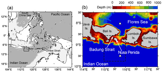
Figure 1.
(a) Overview of the Indonesian archipelago and Indonesian Sea. The area around the Lombok Strait, indicated by black rectangles, is enlarged in (b). In (b), the color contour indicates the water depth. Depths deeper than 1000 m are indicated by the same color (blue). The black dashed line indicates the area focused on this study. The two white triangles indicate the representative positions of the Flores Sea and Indian Ocean to show the difference between the sea surface temperatures (SSTs) at these two positions in Figure 2.
This study focuses on the short-term variation of the SST on a relatively clear day from 20:00 on 27 August 2017 to 5:00 on 28 August 2017. This period covers the semi-diurnal tide (e.g., 12.42 h of the M2 constituent). During the northern summer, the southeasterly monsoon causes the southwestward Ekman transport, which induces coastal upwelling along the southern side of Nusa Tenggara and coastal downwelling along the northern side [28,29]. The coastal upwelling decreases the SST along the southern side of Nusa Tenggara. Figure 2 shows the monthly SST at pixels on the Flores Sea and Indian Ocean in 2017. In the northern summer, a relatively large temperature difference is found between these SSTs (about 2 C in August 2017; larger than the Himawari-8 SST uncertainty). In addition, the general flow pattern through the Lombok Strait is from the Flores Sea to the Indian Ocean in the northern summer [23]; this is due to the ITF, which is the strongest in the northern summer (e.g., [23]). Therefore, we describe how the high-SST water from the Flores Sea intrudes into the Indian Ocean during the northern summer.
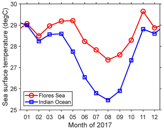
Figure 2.
Monthly SST in the Flores Sea and Indian Ocean in 2017. The representative position of the Flores Sea is 115.45 E and 8 S, and that of the Indian Ocean is 115.45 E and 9.5 S (shown as the white triangles in Figure 1b).
2.2. Maximum Cross-Correlation Method
The MCC method was applied to the sequential Himawari-8 SST images in order to draw the surface current velocity fields. The MCC method is simple in principle and has been widely used to retrieve the surface currents from sequential satellite images such as the SST and ocean color (e.g., [9,10,11,12,13]). The specific procedure is as follows. First, we prepare two consecutive SST images. In the first image, we focus on the SST pattern over an area consisting of several pixels in both the x- and y-directions. The focused pixels of the SST are referred to as the “template.” Then, we find where an SST pattern similar to the template is located in the second image. Specifically, for a template centered at , we compute the normalized cross-correlation between the template and the sub-image centered at in the second image for various p and q [10]:
Here, i and j are the index of the pixels in the x- and y-directions; is the SST in the template centered at and is the SST of the sub-image of the second image; the overline indicates the mean of the SST in the template or sub-image; is the standard deviation of the SST in the template, and is the standard deviation of the SST of the sub-image centered at ; the sigma symbol represents the summation of all of the pixels (i.e., i and j) in the template or sub-image; and n is the number of the pixel in the template or sub-image. The displacement of the template corresponds to the (), where the cross-correlation reaches the maximum. We can then estimate the current velocity due to advection by , where and are the pixel intervals in the x and y directions, respectively; and is the time interval of the two consecutive SST images. Performing the same procedure for the templates centered at various x and y, one can draw the current velocity field.
In this study, the MCC method is applied to the hourly Himawari-8 SST. In general, the MCC method is appropriate for sequential images with a time interval of four to nine hours (e.g., [11,14]). In the area south of the Lombok Strait, however, an interval of one hour would be sufficient because the surface current is strong and the horizontal displacement in one hour corresponds to several pixels.
The SST data were first smoothed, and small-scale image noise was reduced using a two-dimensional Gaussian filter ( pixels with a standard deviation of one pixel). Then, the pixel resolution of 2 km was increased to about 1 km by linear interpolation. With this pixel resolution, the minimum velocity in the estimate (i.e., discretization error) was about 0.28 .
There are three additional important parameters when applying the MCC method: (1) the size of the template, (2) the size of the searching area, and (3) the acceptance criterion of the cross-correlation value. We chose pixels (about 225 km) as the template size, considering the spatial scale of the SST variation. The sides of the search area for the sub-image were 11 km to the south, 5 km to the west, 4 km to the east, and 3 km to the north. The uneven lengths of the sides of the search area were because the southward velocity component was larger than those in the other directions. A search area with a size of 11 km in the southern direction could cover a southward current of up to 3.1 . The acceptance criterion was determined by following a previous study [9], which determined the criterion using a statistical significance test. In this study, cross-correlation values smaller than 0.85 were ignored.
The MCC method assumes that the SST patterns are solely advected and tracks the SST patterns between sequential images using the cross-correlation. South of the Lombok Strait, the SST variation due to advection dominates the variation caused by mixing and diffusion; therefore the MCC method is applicable. Heat flux through the sea surface has a relatively large spatial scale and would affect the SST equally over all pixels in the template and search area; therefore the normalized cross-correlation is likely not affected by the effect of the surface heat flux. However, the limitation of the MCC method is that it cannot accurately estimate the velocity component in directions parallel to the isotherms. Therefore, we focus on the southward velocity of the warm thermal plume (see the Results section below). The flow direction is nearly perpendicular to the isotherms at the southern head of the thermal plume.
3. Results
Figure 3 and Figure 4 show hourly SST fields in the area south of the Lombok Strait. As the general SST pattern, it is clear that Flores Sea water with a high SST (over 27 C) flowed into the Indian Ocean through both passages, forming warm thermal plumes. The SST of the thermal plume from the main passage is higher than that from the Badung Strait. The lower SST of the Badung Strait might be due to river discharge and vertical mixing in the shallow area, which has a strong current. The current inside the Lombok Strait is stronger in the western part than in the eastern part [23]. Although the thermal plume from the Badung Strait flows mainly southward, that from the main passage flows mainly in the south-southwest direction in the Indian Ocean. The SST patterns also show that the cold SST water at the south of Nusa Penida and Bali Island flows southward as well.
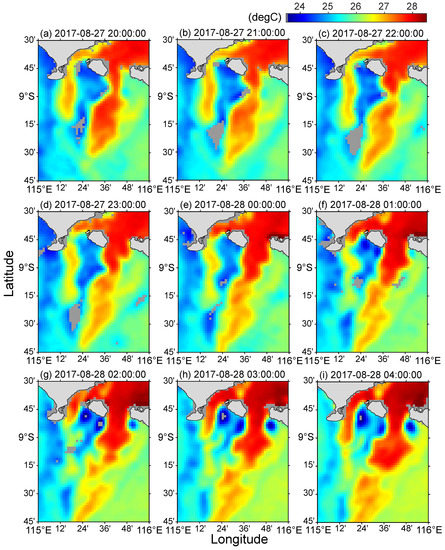
Figure 3.
Hourly SST fields in the area south of the Lombok Strait from (a) 20:00 on 27 August 2017 to (i) 4:00 on 28 August 2018. The gray pixels indicate no SST data for those pixels because of cloud or land.
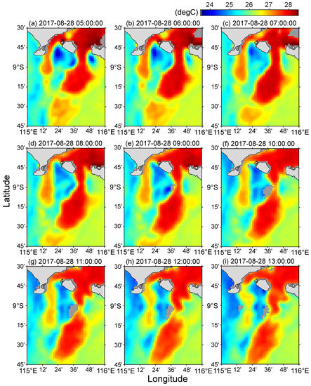
Figure 4.
Same images as Figure 3 but for the periods from (a) 5:00 to (i) 13:00 on 28 August 2017.
The SST to the south of Nusa Penida and Lombok temporarily decreases during certain periods (see Figure 3g–Figure 4a). Such low-SST water moves northward and intrudes into the Lombok Strait from the eastern side of the two passages (see Figure 4b–d), decreasing the SST on the east side of the two passages. The intrusion of low-SST water is more conspicuous in the Badung Strait. As a result of the northward intrusion, the warm water flowing into the Indian Ocean forms a new thermal plume (Figure 3c–e and Figure 4g–i). This short-term flow variation may be due to the tides, which are more active in the Indian Ocean than in the Flores Sea (e.g., [30]). The time difference between the two new warm thermal plumes corresponds closely to the period of the semi-diurnal tide (about 12 h). The warm SST patch that splits from the thermal plume moves southward while deforming its shape. The warm SST patch from the main passage of the Lombok Strait is clearly seen, even at a distance 100 km south of the Lombok Strait.
Figure 5 shows the surface current velocity field estimated by applying the MCC method to the SST images of Figure 3 and Figure 4. In Figure 5, two isotherms of 26 C and 27 C are also shown. Blank locations without an arrow indicate that velocity data do not exist because of clouds or a low cross-correlation value. The estimated velocity of the surface current explains the displacements of the isotherms (from blue to red lines) at the head of the warm thermal plume and of the warm SST patch that split from it. The relatively low SST water to the south of Bali and Nusa Penida flows southward, although the flow patterns of the low-SST water near the Nusa Penida (further north than 9.25 S) are not clear. Current speeds of about 2 are found around the southern head of the warm thermal plume and the warm SST patch that is flowing southward. The warm SST patch keeps its southward speed, even when it is 100 km south of the Lombok Strait (near 9.75 S; see, for example, Figure 5h).
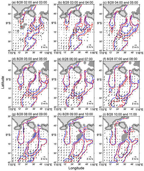
Figure 5.
Surface current velocity fields estimated by applying the MCC method to the sequential SST images of Figure 3 and Figure 4. The results shown are obtained from the SST images from 2:00 to 11:00 on 28 August 2017. In each panel, the blue and red lines are isotherms of 26 C and 27 C of the first and next SST images, respectively.
The spatial and temporal variations of SST were small within the Lombok Strait, and the estimated current velocity would be uncertain inside the strait. For example, when the thermal plume advected southward (see Figure 5a,b), we expected a strong current around the narrowest part of the main passage, considering the continuity of flow. However, the estimated current velocity shows small current there (Figure 5a,b) likely because the temperature gradient is small in the high SST water from the north. The MCC method showed the large current velocity around the main passage only when a new thermal plume was formed (Figure 5i). The maximum velocity was about 2.8 . Because the velocity obtained by the MCC method is an average velocity of the template (225 km in this study), the maximum speed at a particular location can be greater than 2.8 .
4. Discussion
We used the hourly variation of the Himawari-8 SST to gain knowledge of the characteristics of the surface current. Basic spatial SST patterns observed by satellites can also be observed through a series of CTD (conductivity, temperature, and depth) measurements using a research vessel, if the spatial coverage of the survey area are limited. Murray et al. (1990) examined the spatial pattern of the thermal plume around the Lombok sill (excluding the Badung Strait) by CTD measurements [25]. They observed a strong temperature gradient at the west side of the thermal plume. In the Himawari-8 SST, a strong SST gradient is also found at the west side of the thermal plume (Figure 3g–i). The dense data coverage of Himawari-8 SST in both time and space is a great advantage over a series of CTD measurements. While the water property maps (such as temperature maps at some depths) drawn by CTD measurements include the uncertainty due to the time lags of each CTD cast, the satellite SST maps do not include such uncertainty. Using the hourly Himawari-8 SST, we could find the temporal variation of the thermal plume and the warm SST patch that split from it. It would be hard task to capture similar temporal variation of the thermal plume using a series of CTD measurement. Note that CTD measurements are still important because they contain subsurface information and enable discussion on water mass origin (e.g., [31,32]).
We estimated the surface current velocity by applying the MCC method to the hourly Himawari-8 SST. Around the main passage, our estimates suggested that the maximum southward speed reaches about 3 m/s when a new thermal plume is formed. This strong current consists of the tidal current and the ITF. Previous in situ observations of the current velocity have shown that the maximum tidal current exceeds 3 m/s at the Lombok sill (the shallowest area in the main passage) and ranges 0.2 to 0.5 m/s in the northern area of the strait [21,25], and that the surface current of the ITF ranges 0.5 to 1 m/s in the northern summer (e.g., [21,23,26]). Although the MCC method estimated the strong current of the tidal current and ITF, it was unable to separate the two contributions. To separate the two contributions, we need to estimate the current continuously over the period of the M tidal constituent (12.42 h). However, present results appear to underestimate the flow for a period because of the small SST variation around the main passage. It is necessary to improve the tracking technique of the MCC method when applying it to SSTs with small spatial and temporal variations.
In the area south of the Lombok Strait, our estimates suggest that the thermal plume and the warm SST patch that split from the plume flow south–southwestward, with a speed of about 2 m/s. We are unaware of any in situ observations that measured the current velocity of this thermal plume flowing southward. Some numerical ocean models do show the southward outflow from the Lombok Strait (e.g., [33,34]). Since these models do not include tides, our estimates of the southward speed cannot be quantitatively compared with the simulated flow. However, the directions of current velocity of these models are mainly south–southwestward [33,34] and agree with this study. The agreement of the current velocity direction supports the results of the numerical models.
One of the oceanic current systems relating to the south of the Lombok Strait is the South Java Current (SJC), which flows along the south of Java Island and is driven primarily by winds (e.g., [33]). The SJC flows eastward along the south of Java in August [35]. The SJC has a relatively cold signature, and the low-SST water at the south of Bali corresponds to the SJC in the study period. An eastward velocity was continuously observed at the Ombai Strait (Figure 1) over the year, which led Sprintall et al. (2010) to suggest that the SJC reaches the Ombai Strait nearly all year round [36]. However, the Himawari-8 SST shows that the relatively cold signature of the SJC near the surface is discontinuous south of the Lombok Strait because of the thermal plume advecting southward from the strait. The discontinuity of the cold SST south of the Lombok Strait is also found in the Himawari-8 monthly SST and also in the monthly SST atlas, which was produced using the SST product observed by AVHRR [37]. The estimated flow field suggests that the surface flow of the SJC is directed southward together with the outflow from the Lombok Strait and possibly becomes a part of the Indian South Equatorial Current flowing westward at around 13 S. The eastward surface current observed at the Ombai Strait in the northern summer [36] is unlikely to be the one continuously flowing from the south of Java. Note, however, that the Himawari-8 provides surface information only; how the SJC behaves at the subsurface requires a more detailed discussion based on subsurface information.
5. Conclusions
The hourly Himawari-8 SST was used to gain knowledge of the characteristics of the surface current in the area south of the Lombok Strait. The intrusion of Flores Sea water into the Indian Ocean was clearly observed in the form of the warm thermal plume, not only from the main passage of the Lombok Strait but also from the Badung Strait. The short-term variation associated with the tide was also observable in the hourly Himawari-8 SST; the relatively cold water south of Lombok and Nusa Penida intruded into the Lombok Strait for a certain period, although this northward intrusion was very minor compared to the intrusion of Flores Sea water into the Indian Ocean. Due to this northward intrusion, the thermal plume appears to split repeatedly following the tidal cycle (about 12 h). The warm SST patch that split from the thermal plume advected south–southwestward while deforming its shape. The warm SST patch was clearly seen even at a distance 100 km south of the Lombok Strait.
The maximum cross-correlation (MCC) method was applied to the hourly Himawari-8 SST to estimate the surface current velocity. In the area south of the Lombok Strait, a current speed of about 2 was commonly found around the southern head of the warm thermal plume and warm SST patch flowing south–southwestward. This outflow from the Lombok Strait kept its southward speed even at a distance 100 km south of the strait. At the Lombok sill, the present MCC method was able to estimate strong currents only when a new thermal plume was formed. Nonetheless, the estimated speed was in agreement with previous in situ observations.
This study focused on the flow patterns south of the Lombok Strait, which is one of the main paths of the ITF. The ITF is the only flow that connects the Pacific and Indian oceans near the equator, making the Lombok Strait one of the most important regions in oceanography. However, its close proximity to land and various islands have made it hard to directly observe its flow field. We have shown that the satellite SST provides rich information about this flow, not only on temperature but also on the flow field. Although subsurface information is also required for estimating the total heat and volume transport of the ITF, the spatial distribution of the SST and the surface flow field provide a useful reference that would supplement other observations and modeling studies. Finally, although we focused on the SST around the Lombok Strait in this study, satellite SSTs can be used to capture flow patterns in the entire Indonesian Sea and design an effective means of observation for the ITF.
Author Contributions
Conceptualization and methodology, Y.S., H.M., and F.S.; formal analysis and visualization, N.T.; supervision, Y.S. and S.K.; investigation and writing—original draft preparation, N.T., and S.K.; writing—review and editing, all authors.
Funding
This work was supported by JSPS KAKENHI Grant Number 17H04625, 17H03494, 18H03731, 19H04292.
Acknowledgments
The SST product (produced from Himawari-8) used in this paper was supplied by the P-Tree System (https://www.eorc.jaxa.jp/ptree/userguide.html) of JAXA.
Conflicts of Interest
The authors declare no conflict of interest.
References
- Johannessen, O.M.; Sandven, S.; Jenkins, A.D.; Durand, D.; Pettersson, L.H.; Espedal, H.; Evensen, G.; Hamre, T. Satellite earth observation in operational oceanography. Coast. Eng. 2000, 41, 155–176. [Google Scholar] [CrossRef]
- Lee, T.; McPhaden, M.J. Increasing intensity of El Niño in the central-equatorial Pacific. Geophys. Res. Lett. 2010, 37. [Google Scholar] [CrossRef]
- Wentz, F.J.; Gentemann, C.; Smith, D.; Chelton, D. Satellite Measurements of Sea Surface Temperature Through Clouds. Science 2000, 288, 847–850. [Google Scholar] [CrossRef] [PubMed]
- Ray, R.D.; Susanto, R.D. Tidal mixing signatures in the Indonesian seas from high-resolution sea surface temperature data. Geophys. Res. Lett. 2016, 43, 8115–8123. [Google Scholar] [CrossRef]
- Klemas, V. Remote Sensing of Coastal and Ocean Currents: An Overview. J. Coast. Res. 2012, 28, 576–586. [Google Scholar] [CrossRef]
- Ducet, N.; Le Traon, P.Y.; Reverdin, G. Global high-resolution mapping of ocean circulation from TOPEX/Poseidon and ERS-1 and -2. J. Geophys. Res. Ocean. 2000, 105, 19477–19498. [Google Scholar] [CrossRef]
- Scharffenberg, M.G.; Stammer, D. Seasonal variations of the large-scale geostrophic flow field and eddy kinetic energy inferred from the TOPEX/Poseidon and Jason-1 tandem mission data. J. Geophys. Res. Ocean. 2010, 115. [Google Scholar] [CrossRef]
- Kelly, K.A. An Inverse Model for Near-Surface Velocity from Infrared Images. J. Phys. Oceanogr. 1989, 19, 1845–1864. [Google Scholar] [CrossRef]
- Emery, W.J.; Thomas, A.C.; Collins, M.J.; Crawford, W.R.; Mackas, D.L. An objective method for computing advective surface velocities from sequential infrared satellite images. J. Geophys. Res. Ocean. 1986, 91, 12865–12878. [Google Scholar] [CrossRef]
- Garcia, C.A.E.; Robinson, I.S. Sea surface velocities in shallow seas extracted from sequential coastal zone color scanner satellite data. J. Geophys. Res. Ocean. 1989, 94, 12681–12691. [Google Scholar] [CrossRef]
- Tokmakian, R.; Strub, P.T.; McClean-Padman, J. Evaluation of the Maximum Cross-Correlation Method of Estimating Sea Surface Velocities from Sequential Satellite Images. J. Atmos. Ocean. Technol. 1990, 7, 852–865. [Google Scholar] [CrossRef]
- Wahl, D.D.; Simpson, J.J. Physical processes affecting the objective determination of near-surface velocity from satellite data. J. Geophys. Res. Ocean. 1990, 95, 13511–13528. [Google Scholar] [CrossRef]
- Chubb, S.R.; Mied, R.P.; Shen, C.Y.; Chen, W.; Evans, T.E.; Kohut, J. Ocean Surface Currents From AVHRR Imagery: Comparison With Land-Based HF Radar Measurements. IEEE Trans. Geosci. Remote. Sens. 2008, 46, 3647–3660. [Google Scholar] [CrossRef]
- Heuzé, C.; Carvajal, G.K.; Eriksson, L.E.B. Optimization of Sea Surface Current Retrieval Using a Maximum Cross-Correlation Technique on Modeled Sea Surface Temperature. J. Atmos. Ocean. Technol. 2017, 34, 2245–2255. [Google Scholar] [CrossRef]
- Ryu, J.H.; Han, H.J.; Cho, S.; Park, Y.J.; Ahn, Y.H. Overview of geostationary ocean color imager (GOCI) and GOCI data processing system (GDPS). Ocean. Sci. J. 2012, 47, 223–233. [Google Scholar] [CrossRef]
- Bessho, K.; Date, K.; Hayashi, M.; Ikeda, A.; Imai, T.; Inoue, H.; Kumagai, Y.; Miyakawa, T.; Murata, H.; Ohno, T.; et al. An introduction to Himawari-8/9—Japan’s new-generation geostationary meteorological satellites. J. Meteorol. Soc. Jpn. Ser. II 2016, 94, 151–183. [Google Scholar] [CrossRef]
- Warren, M.A.; Quartly, G.D.; Shutler, J.D.; Miller, P.I.; Yoshikawa, Y. Estimation of ocean surface currents from maximum cross correlation applied to GOCI geostationary satellite remote sensing data over the Tsushima (Korea) Straits. J. Geophys. Res. Ocean. 2016, 121, 6993–7009. [Google Scholar] [CrossRef]
- Wyrtki, K. Indonesian through flow and the associated pressure gradient. J. Geophys. Res. Ocean. 1987, 92, 12941–12946. [Google Scholar] [CrossRef]
- Meyers, G. Variation of Indonesian throughflow and the El Niño-Southern Oscillation. J. Geophys. Res. Ocean. 1996, 101, 12255–12263. [Google Scholar] [CrossRef]
- Gordon, A.L. Oceanography of the Indonesian Seas and Their Throughflow. Oceanography 2005, 18, 14–27. [Google Scholar] [CrossRef]
- Murray, S.P.; Arief, D. Throughflow into the Indian Ocean through the Lombok Strait, January 1985–January 1986. Nature 1988, 333, 444. [Google Scholar] [CrossRef]
- Gordon, A.L.; Susanto, R.D.; Ffield, A.; Huber, B.A.; Pranowo, W.; Wirasantosa, S. Makassar Strait throughflow, 2004 to 2006. Geophys. Res. Lett. 2008, 35. [Google Scholar] [CrossRef]
- Sprintall, J.; Wijffels, S.E.; Molcard, R.; Jaya, I. Direct estimates of the Indonesian Throughflow entering the Indian Ocean: 2004–2006. J. Geophys. Res. Ocean. 2009, 114. [Google Scholar] [CrossRef]
- Iskandar, I.; Masumoto, Y.; Mizuno, K.; Sasaki, H.; Affandi, A.K.; Setiabudidaya, D.; Syamsuddin, F. Coherent intraseasonal oceanic variations in the eastern equatorial Indian Ocean and in the Lombok and Ombai Straits from observations and a high-resolution OGCM. J. Geophys. Res. Ocean. 2014, 119, 615–630. [Google Scholar] [CrossRef]
- Murray, S.P.; Arief, D.; Kindle, J.C.; Hurlburt, H.E. Characteristics of Circulation in an Indonesian Archipelago Strait from Hydrography, Current Measurements and Modeling Results. In The Physical Oceanography of Sea Straits; Pratt, L.J., Ed.; Springer: Dordrecht, The Netherlands, 1990; pp. 3–23. [Google Scholar] [CrossRef]
- Hautala, S.L.; Sprintall, J.; Potemra, J.T.; Chong, J.C.; Pandoe, W.; Bray, N.; Ilahude, A.G. Velocity structure and transport of the Indonesian Throughflow in the major straits restricting flow into the Indian Ocean. J. Geophys. Res. Ocean. 2001, 106, 19527–19546. [Google Scholar] [CrossRef]
- Kurihara, Y.; Murakami, H.; Kachi, M. Sea surface temperature from the new Japanese geostationary meteorological Himawari-8 satellite. Geophys. Res. Lett. 2016, 43, 1234–1240. [Google Scholar] [CrossRef]
- Susanto, R.D.; Gordon, A.L.; Zheng, Q. Upwelling along the coasts of Java and Sumatra and its relation to ENSO. Geophys. Res. Lett. 2001, 28, 1599–1602. [Google Scholar] [CrossRef]
- Kida, S.; Wijffels, S. The impact of the Indonesian Throughflow and tidal mixing on the summertime sea surface temperature in the western Indonesian Seas. J. Geophys. Res. Ocean. 2012, 117. [Google Scholar] [CrossRef]
- Ray, R.D.; Egbert, G.D.; Erofeeva, S.Y. Tides in the Indonesian seas. Oceanography 2005, 18, 74–79. [Google Scholar] [CrossRef]
- Atmadipoera, A.; Molcard, R.; Madec, G.; Wijffels, S.; Sprintall, J.; Koch-Larrouy, A.; Jaya, I.; Supangat, A. Characteristics and variability of the Indonesian throughflow water at the outflow straits. Deep. Sea Res. Part I Oceanogr. Res. Pap. 2009, 56, 1942–1954. [Google Scholar] [CrossRef]
- Bayhaqi, A.; Iskandar, I.; Surinati, D.; Budiman, A.S.; Wardhana, A.K.; Dirhamsyah; Yuan, D.; Lestari, D.O. Water mass characteristic in the outflow region of the Indonesian throughflow during and post 2016 negative Indian ocean dipole event. IOP Conf. Ser. Earth Environ. Sci. 2018, 149, 012053. [Google Scholar] [CrossRef]
- Iskandar, I.; Tozuka, T.; Sasaki, H.; Masumoto, Y.; Yamagata, T. Intraseasonal variations of surface and subsurface currents off Java as simulated in a high-resolution ocean general circulation model. J. Geophys. Res. Ocean. 2006, 111. [Google Scholar] [CrossRef]
- Metzger, E.; Hurlburt, H.; Xu, X.; Shriver, J.F.; Gordon, A.; Sprintall, J.; Susanto, R.; van Aken, H. Simulated and observed circulation in the Indonesian Seas: 1/12° global HYCOM and the INSTANT observations. Dyn. Atmos. Ocean. 2010, 50, 275–300. [Google Scholar] [CrossRef]
- Sprintall, J.; Chong, J.; Syamsudin, F.; Morawitz, W.; Hautala, S.; Bray, N.; Wijffels, S. Dynamics of the South Java Current in the Indo-Australian Basin. Geophys. Res. Lett. 1999, 26, 2493–2496. [Google Scholar] [CrossRef]
- Sprintall, J.; Wijffels, S.; Molcard, R.; Jaya, I. Direct evidence of the South Java Current system in Ombai Strait. Dyn. Atmos. Ocean. 2010, 50, 140–156. [Google Scholar] [CrossRef]
- Wijffels, S.E.; Beggs, H.; Griffin, C.; Middleton, J.F.; Cahill, M.; King, E.; Jones, E.; Feng, M.; Benthuysen, J.A.; Steinberg, C.R.; et al. A fine spatial-scale sea surface temperature atlas of the Australian regional seas (SSTAARS): Seasonal variability and trends around Australasia and New Zealand revisited. J. Mar. Syst. 2018, 187, 156–196. [Google Scholar] [CrossRef]
© 2019 by the authors. Licensee MDPI, Basel, Switzerland. This article is an open access article distributed under the terms and conditions of the Creative Commons Attribution (CC BY) license (http://creativecommons.org/licenses/by/4.0/).