3D Point Cloud Semantic Modelling: Integrated Framework for Indoor Spaces and Furniture

Abstract

3D models derived from point clouds are useful in various shapes to optimize the trade-off between precision and geometric complexity. They are defined at different granularity levels according to each indoor situation. In this article, we present an integrated 3D semantic reconstruction framework that leverages segmented point cloud data and domain ontologies. Our approach follows a part-to-whole conception which models a point cloud in parametric elements usable per instance and aggregated to obtain a global 3D model. We first extract analytic features, object relationships and contextual information to permit better object characterization. Then, we propose a multi-representation modelling mechanism augmented by automatic recognition and fitting from the 3D library ModelNet10 to provide the best candidates for several 3D scans of furniture. Finally, we combine every element to obtain a consistent indoor hybrid 3D model. The method allows a wide range of applications from interior navigation to virtual stores.

1. Introduction

3D point cloud geometric depiction is implemented in many 3D modelling techniques to best represent underlying shapes. This need is driven by applications in numerous industries—architecture, construction, engineering and facility management; Risk assessment and emergency planning; Simulations; Marketing; Entertainment; Robotics; Transportation and mobility—for tasks such as structural deformation scenarios [1,2], quality and progress control [3], or even for asset creation in the entertainment business [4,5]. To extend this range of applications, the data mining and processing research communities have focused on adding additional information to the 3D model through semantic descriptors [6]. This in turn leads to more advanced uses of 3D virtual data, of which many have indoor scenario benefits. For instance, we employ 3D semantic models to plan/monitor emergency routes [7,8,9,10,11], for serious gaming [12,13], 3D wave propagation simulations [14,15,16,17], localization of safety-relevant features [18], virtual museums [19], and product lifecycle management [20]. More recently, the field of robotics has demonstrated a great interest in these enhanced 3D geometries for creation [21,22], scan planning [23], and for 3D autonomous indoor navigation [24,25,26] with regard to transportation and mobility problematics [27]. However, bridging the gap between point cloud data, 3D models and semantic concepts is a very complicated task which usually requires a good knowledge of the specific application domain.

Our contribution is an attempt to narrow this gap by leveraging formalized knowledge and expert systems [28] based on point clouds. We want to take advantage of computer reasoning over semantic representations of our environment. However, this demands highly challenging knowledge processing due to the heterogeneity of the application domains and the various 3D representations.

Our approach addresses Knowledge Extraction (KE), Knowledge Integration (KI) and Knowledge Representation (KR) [29] to better assimilate point cloud data of various quality [30]. Indeed, most software and tools existing in our computerized environment were developed to work primarily with 3D models. The landscape in standards, practices and usages is mostly established for these representations. This motivates a flexible and modular infrastructure, for which point clouds can be the starting point [31,32,33,34], allowing interoperable and two-way exchanges (from and to the point cloud enrichment frameworks). If enhanced with additional information (geometry/topology/semantics), they could be used for deriving more representative 3D shapes and to provide a higher compatibility with 3D modelling workflows. As such, we need new methods that can directly derive application-driven 3D semantic representations while conserving interoperability over centralized semantics. This hypothesis considers point clouds to be semantically rich (i.e. it contains semantics linking group of points together, such as segment or class information) and efficiently organized for various processing tasks.

While the present paper is based on the Smart Point Cloud (SPC) Infrastructure [31], it can be replicated over any segmented dataset that benefits from different sets of attribute information. The main idea is that, based on a 3D point cloud describing an indoor environment, we can extract 3D models of each object instance with regard to an application ontology and combine them to generate tailored 3D representations suited for specific indoor scenarios. To provide a multi-LoD framework for different utilizations, we support the modelling process with a characterization mechanism that can deepen the geometric analysis of shapes. We study the structuring and reasoning aptitude of ontologies for pulling contextual information and enhancing the modelling fit. Thus, we explore the possibility of leveraging formalized knowledge to recreate occluded areas and to infer non-existent geometries. Our approach is extended with a 3D shape-matching approach through data mining using the 3D library ModelNet10 [35]. The end goal of this contribution is to derive a comprehensive 3D model extended with semantic information. In this paper, we focus on indoor reconstructions and asset management.

In the first part (Section 2), we review significant related work studying 3D point cloud modelling approaches and several use cases in which they were successfully employed. Driven by this state of the art, we then present in Section 3 our designed 3D reconstruction framework following a part-to-whole outline. We finally describe the results (Section 4), looking at the precisions and performances for different datasets. Based on a critical analysis, we provide the main findings, the limitations and the perspectives (Section 5) that the approach brings to 3D point cloud modelling of building interiors.

2. Related Work

In this section, we briefly review most recent methods for point cloud modelling. We organize the related works as follows: Section 2.1 includes recent methods for geometric reconstruction based on indoor point clouds; Section 2.2 describes instance-based recognition, featuring and model fitting; and Section 2.3 describes knowledge integration for object relationship modelling.

2.1. Methods for 3D Point Cloud Geometric Modelling

3D reconstruction from indoor point cloud data gravitates around different approaches for automatic modelling with different granularities. The chosen method is often guided by the application needs in term of precision, resolution, complexity and completeness. For example, semantic model utilizations [36] include the creation of as-built models for the monitoring of construction processes, while visually appealing virtual models of historical sites enable immersive experiences. While the latter emphasize high-quality visuals, semantic applications often rely on approximate reconstructions of the global scene which convey the object arrangement. Both semantic and virtual indoor 3D models can be extended using precise metric information to provide key information for public buildings or to assist indoor navigation. Several works address these different characteristics through shape representation, which has been extensively studied in the last century. Generally, we look for perceptually important shape features in either the shape boundary information, or the boundary plus interior content, as noted in [37].

We can primarily distinguish between explicit and implicit shape representations. Explicit representations translate the shape of an object (e.g., a triangle mesh), while implicit representations indirectly encode the shape using a set of features (histograms, normal, curvature, etc.). Explicit representations are well suited for modelling 3D objects, whereas implicit representations are most often used for 3D object recognition and classification [38]. In most reviews, point cloud modelling approaches are categorized regarding the type of representation, the type of input data or the type of algorithms used. In this section, we will study the algorithms depending on their context and available information, similar to F. Remondino in [39].

3D reconstructions that make use only of the spatial attributes within point cloud data are found in many works. Delaunay-based methods are quite common in this area, and we invite the reader to study [40] for a comprehensive survey of these methods. These approaches place rather strong requirements on the data and are impractical for scanned real-world scenes containing significant imperfections. Also, it is often necessary to optimize the polycount (total number of triangular polygons it takes to draw the model in 3D space) for memory efficiency. As such, quad meshing [41] can lighten the representation and smoothness. A practical example of Boundary-Representation (B-Rep) can be found in Valero et al. [42] for the reconstruction of walls. While these are interesting for their low input requirements, we investigate techniques more fitted toward dealing with challenging artifacts such as occlusion. Berger et al. [43,44] propose an exhaustive state-of-the-art surface reconstruction from point clouds. They reviewed thirty-two point cloud modelling methods by comparing their fit to noisy data, missing data, non-uniform sampling, and outliers, but also their requirements in terms of input features (normal, RGB data, scan data, etc.) and shape class (CAD, indoor, primitives, architectural, etc.). While surface smoothness approaches such as tangent planes, Poisson and Graph-Cut [44] can quickly produce a mesh, they often lack robustness to occlusion and incompletion. Sweeping models, primitive instancing, Whitney regular stratification or Morse decompositions [45] may be used for applications in robot motion planning and generally provide a higher tolerance for missing data.

Primitives are good candidates for indoor modelling with a high generalization potential, a low storage footprint and many application scenarios. Indeed, as noticed by the authors in [46], parametric forms are “mathematically complete, easily sampled, facilitate design, can be used to represent complex object geometries and can be used to generate realistic views”. They describe a shape using a model with a small number of parameters (e.g., a cylinder may be represented by its radius, its axis, and the start and end points). They can also be represented non-parametrically or converted through the process of tessellation. This step is used in polygon-based rendering, where objects are broken down from abstract primitive representations to meshes. As noted by authors in [47], indoor environments are often composed of basic elements, such as walls, doors, windows, furniture (chairs, tables, desks, lamps, computers, cabinets) which come from a small number of prototypes and repeat many times. Such building components are generally formed of rigid parts whose geometries are locally simple (they consist of surfaces that are well approximated by planar, cylindrical, conical and spherical shapes.). An example is given in the work of Budroni and Boehm [48], where the authors model walls by fitting CAD primitives. Furthermore, although variability and articulation are central (a door swings, a chair is moveable or its base rotates), such changeability is often limited and low dimensional. Thus, simple shapes are extensively used in the first steps of as-built modelling due to their compactness and the low number of parameters allowing efficient fitting methods [49]. For more complex shapes, explicit parametric representations are still available (e.g., Bézier curves, B-spline, NURBS) but they are mostly used as design tools. Since their control points cannot easily be inferred from point cloud data, these representations are rarely used in shape analysis. An example of parametric collection is given by Lee et al. [50]. They propose a skeleton-based 3D reconstruction of as-built pipelines from laserscan data. The approach allows the fully automated generation of as-built pipelines composed of straight cylinders, elbows, and tee pipes directly fitted. While the method provides good results, its specificity restrains a possible generalization. Fayolle and Pasko [51] highlight the interaction potential given by parametrized objects within indoor environments. Indeed, through a clever binary CSG (Constructive Solid Geometry) or n-ary (FRep) construction tree structure, they store object-relations such that the user could modify individual parts impacting the entire logic of the object construction, including its topology. Such a parametrized model reconstruction is required in many fields, such as mechanical engineering or computer animation. Other relevant works highlight the papers of Fathi et al. [36] for civil infrastructure reconstruction, or Adan and Huber [52], which provides a 3D reconstruction methodology (wall detection, occlusion labelling, opening detection, occlusion reconstruction) of interior wall surfaces which is robust to occlusion and clutter. Both results are a primitive-based assembly based on these surfaces.

While parametric assemblage gives a lot of flexibility, in some cases, such as for highly complex shapes, there is a need for low geometric modelling deviations. In such scenarios, non-parametric representations such as polygonal meshes are employed to better fit the underlying data. However, the lack of compactness of these representations limits their use, especially when dealing with large point clouds. Hence, using a combination of both representations is advisable when a global representation is required. In such approaches, parametric representations are usually used as local representations and decomposed into parts (e.g., using CSG to represent each part with one or more geometric primitives). In contrast, triangle meshes are flexible enough to be used as global representations, since they can describe free-form objects in their entirety [38]. For example, Stamos et al. [53] present such a 3D modelling method on a church environment by combining planar segments and mesh elements. Using a different approach, Xiao and Furukawa [19] propose the “Inverse CSG” algorithm to produce compact and regularized 3D models. A building is sliced, and for each slice, different features (free space constraint, line extraction, iterative 2D CSG model reconstruction) are extracted, stacked and textured to obtain a 3D model of walls. The method is interesting for its approach to leveraging 2D features and its noise robustness, but it will not process complex structures, furniture or non-linear walls. Other hybrid approaches introduced knowledge within workflows to try to overcome the main challenges, especially missing data. A significant work was published by Lafarge et al. [54], which develops a hybrid modelling process where regular elements are represented by 3D primitives whereas irregular structures are described by mesh-based surfaces. These two different types of 3D representation interact through a non-convex energy minimization problem described in [55]. The approach successfully employed for large outdoor environments shows the benefits of leveraging semantics for better point cloud fitting. The authors in [56] present a reverse engineering workflow based on a hybrid modelling approach while also leveraging knowledge. They propose a linear modelling approach through cross-section of the object by fitting splines to the data and then sweeping the cross-section along a trajectory to form the object model. To realize such operations, they first extracted architectural knowledge based on the analysis of architectural documents to be used for guiding the modelling process. An example illustrated in [57] provides a method to reconstruct the boundaries of buildings by extracting walls, doors, roofs and windows from façade and roofs point clouds. The authors use convex or concave polygons adjusted to different features separately. Interestingly, we note that the authors use knowledge to generate assumptions for the occluded parts. Finally, all polygons are combined to generate a polyhedron model of a building. This approach is interesting for its whole-to-part consideration, which leverages knowledge to optimize the ratio approximation/compactness.

While triangulation and hybrid modelling can be successfully used for various indoor scenarios, we notice that the most prominent module is the parametric modelling method. Its fit to both B-Rep and volumetric modelling accompanied by its high flexibility in representativity at different granularity levels will thus be further investigated in Section 3. Also, we notice that in some works, the use of knowledge makes it possible to better describe shapes when used within the modelling workflow. We will thus investigate the literature for KI and KR in Section 2.3.

2.2. Instance-Based Object Recognition and Model Fitting

Man-made objects populating indoor scenes often have low degrees of freedom and are arrangements of simple primitives. Beneath representation and compression efficiency [53,54,55], there is a real need to independently model different objects of interest that can in turn host different relationship information. The process of instance-based object recognition is required for identifying objects with a known shape, or objects that are repeated throughout a facility. The predominance of primitive forms in these environments gives specific shape descriptors major control over the implicit representation. These can be categorized as geometric feature descriptors and symmetric feature descriptors. In many works, we find that planar detection plays a predominant role for the detection of elements in KE, specifically segmentation workflow.

Geometric feature descriptors: As such, predominant algorithms for geometric featuring in scientific literature are RANSAC [58,59,60,61,62,63,64,65,66], Sweeping [67], Hough [68,69,70,71] and PCA [61,72,73,74,75,76,77]. The authors [61,78] provide a robust PCA approach for plane fitting. The paper by Sanchez [63] primarily makes use of RANSAC to detect most building interiors, that may be modelled as a collection of planes representing ceilings, floors, walls and staircases. Mura et al. [79] partitions an input 3D model into an appropriate number of separate rooms by detecting wall candidates and then studying the possible layout by projecting the scenarios in a 2D space. Arbeiter et al. [80] present promising descriptors, namely the Radius-Based Surface Descriptor (RSD), Principal Curvatures (PC) and Fast Point Feature Histograms (FPFH). They demonstrate how they can be used to classify primitive local surfaces such as cylinders, edges or corners in point clouds. More recently, Xu et al. [81] provide a 3D reconstruction method for scaffolds from a photogrammetric point cloud of construction sites using mostly point repartitions in specific reference frames. Funkhouser et al. [82] also propose a matching approach based on shape distributions for 3 models. They pre-process through random sampling to produce a continuous probability distribution later used as a signature for each 3D shape. The key contribution of this approach is that it provides a framework within which arbitrary and possibly degenerate 3D models can be transformed into functions with natural parameterizations. This allows simple function comparison methods to produce robust dissimilarity metrics and will be further investigated in this paper.

We find that using other sources of features both from analytical workflows as well as domain knowledge can contribute heavily to better segmentation workflows or for guiding 3D modelling processes.

Symmetry feature descriptors: Many shapes and geometrical models show symmetries—isometric transforms that leave the shape globally unchanged. If one wants to extract relationship graphs among primitives, symmetries can provide valuable shape descriptions for part modelling. In the computer vision and computer graphics communities, symmetry has been identified as a reliable global knowledge source for 3D reconstruction. The review in [83] provides valuable insights on symmetry analysis both at a global and local scale. It highlights the ability of symmetries to extract features better, describing furniture using a KR, specifically an ontology. In this paper, the extracted symmetric patches are treated as alphabets and combined with the transforms to construct an inverse-shape grammar [84]. The paper of Martinet et al. [85] provides an exhaustive review of accurate detection of symmetries in 3D Shapes. These are used for planar and rotational symmetries in Kovacs et al. [86] to define candidates’ symmetry planes for perfecting CAD models by reverse engineering. The paper is very interesting for its ability to leverage knowledge about the shape symmetries. Adan and Huber [52] list façade reconstruction methods, mainly based on symmetry study and reconstitution of planar patches, and then proposes a method that can handle clutter and occluded areas. While they can achieve a partial indoor reconstruction of walls and openings, it necessitates specific scan positions independently treated by ray-tracing. All these features play an important role for implicit geometric modelling, but also in shape-matching methods.

Feature-based shape matching: For example, symmetry descriptors are used to query a database for shape retrieval in [87]. The authors in [88] propose a model reconstruction by fitting from a library of established 3D parametric blocks, and Nan et al. [89] make use of both geometric and symmetric descriptors to best-fit candidates from a 3D database, including a deformable template fitting step. However, these methods often include a pre-segmentation step and post-registration phase, which highly condition the results and constrain the methodology to perfect shapes without outliers or missing data. Following this direction, F. Bosché [90] proposes a method using CAD model fitting for dimensional compliance control in construction. The approach is robust to noise and includes compliance checks of the CAD projects with respect to established tolerances to validate the current state of construction. While the approach permits significant automation, it requires a coarse registration step to be performed by manually defining pair points in both datasets. To automate the registration of models with candidates, the Iterative Closest Point (ICP) method [91] is often used for fine registration, with invariant features in [92], based on least squares 3D surface and curve matching [93], non-linear least squares for primitive fitting [94] or using an energy minimization in graph [95]. The recent works of Xu et al. in [96,97] present a global framework where co-segmented shapes are deformed by scaling corresponding parts in the source and target models to fit a point cloud in a constrained manner using non-rigid ICP and deformation energy minimization. These works are foundations and provide research directions for recovering a set of locally fitted primitives with their mutual relations.

We have seen that knowledge extraction for indoor scenario is mostly driven by three categories of features namely geometric, symmetric and for shape matching. Moreover, object-relationships among the basic objects of these scenes satisfy strong priors (e.g., a chair stands on the floor, a monitor rests on the table) as noted by [47], which motivates the inclusion of knowledge through KI for a better scene understanding and description.

2.3. Knowledge Integration (KI) for Object-Relationship Modelling

3D indoor environments demand to be enriched with semantics to be used in the applications described in Section 1. This has led to the creation of standards such as LADM [98], IndoorGML [99] or IFC (Industry Foundation Class) [100], which were motivated by utilizations in the AEC industry, navigation systems or land administration. Indeed, the different models can deal with semantically annotated 3D spaces and can operate with abstract spaces and subdivision views, and have a notion of geometry and topology while maintaining the relationship between objects. The choice of one model or another is mainly guided by usage and its integration within one community. Therefore, semantically rich 3D models provide a great way to extend the field of application and stresses new ways to extract knowledge a priori for a fully autonomous Cognitive Decision System (CDS). The CDS can, in turn, open up new solutions for industries listed in the Global Industry Classification Standard [101].

In their work, Tang et al. [38] separate this process into geometric modelling, object recognition, and object relationship modelling. Whereas a CAD model would represent a wall as a set of independent planar surfaces, a BIM model would represent the wall as a single, volumetric object with multiple surfaces, as well as adjacency relationships between the wall and other entities in the model, the identification of the object as a wall, and other relevant properties (material characteristics, cost, etc.). This includes topological relationships between components, and between components and spaces. Connectivity relationships indicate which objects are connected to one another and where they are connected. Additionally, containment relationships are used to describe the locations of components that are embedded within one another (e.g., a window embedded within a wall).

Ochmann et al. [69] present an automatic reconstruction of parametric walls and openings from indoor point clouds. Their approach reconstructs walls as entities with constraints on other entities, retaining wall relationships and deprecating the modification of one element onto the other. The authors of [23,102,103,104] extend the processes of the parametric modelling of walls and openings to BIM modelling applications. More recently, the paper by Macher et al. [68] presented a semi-automatic approach for the 3D reconstruction of walls, slabs and openings from a point cloud of a multi-storey building, and provides a proof of concept of OBJ for IFC manual creation. While these approaches have contributed to new possibilities for the semantic modelling of walls and slabs, the object-relationship is limited to topological relationships.

The work of Fisher in [105] introduces domain knowledge of standard shapes and relationships into reverse engineering problems. They rightfully state that there are many constraints on feature relationships in manufactured objects and buildings which are investigated in this paper. Indeed, for a general workflow, one must provide a recovery process even when data is very noisy, sparse or incomplete through a general shape knowledge. Complete data acquisition (impossible in practice for some situations) through inference of occluded data permits the discovery of shape and position parameters that satisfy the knowledge-derived constraints. Formalizing knowledge would therefore be useful to apply known relationships when fitting point cloud data and get better shape parameter estimates. It can also be used to infer data about unseen features, which directs our work to consider ontologies. In this area, the work of Dietenbeck et al. [6] makes use of multi-layer ontologies for integrating domain knowledge in the process of 3D shape segmentation and annotation. While they provide only an example and a manual approach for meshes, they describe an expert knowledge system for furniture in three conceptual layers, directly compatible with the three meta-models of the Smart Point Cloud Infrastructure introduced in [31] and extended in [29]. The first layer corresponds to the basic properties of any object, such as shapes and structures, whereas the upper layers are specific to each application domain and describe the functionalities and possible configurations of the objects in this domain. By using domain knowledge, the authors perform searches among a set of possible objects, while being able to suggest segmentation and annotation corrections to the user if an impossible configuration is reached. This work will be further investigated within our workflow. Using a different approach, Son and Kim [106] present a semantic as-built 3D modelling pipeline to reconstruct structural elements of buildings based on local concavity and convexity. They provide different types of functional semantics and shapes with an interesting parameter calculation approach based on analytic features and domain knowledge. These works are fundamental and greatly illustrate the added benefit of leveraging knowledge.

KI and KR are an important part of any intelligent system. In this review, we noticed that the use of ontologies provided an interesting addition to knowledge formalization and made it possible to better define object-relationships. Coupled with a KE approach treating geometric, symmetric and shape matching features, they could provide a solid foundation for procedural modelling based on a 3D point cloud. Therefore, we develop a method (Section 3) inspired by these pertinent related works.

3. Materials and Methods

In this section, we present a global framework for modelling pre-segmented/classified indoor point cloud data. The approach is divided into four steps, A, B, C, D (as illustrated in Figure 1), respectively described in the four Section 3.1, Section 3.2, Section 3.3 and Section 3.4. The methodology follows a part-to-whole design where each instance is treated separately before aggregation to reconstruct a semantically rich global 3D model.

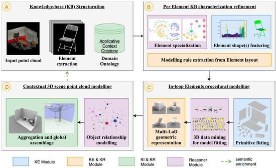
Figure 1. Global workflow for modelling indoor point cloud data. Our approach takes as an input a semantically rich point cloud (A) and uses knowledge-based processes (B–D) to extract a hybrid 3D model.

In Section 3.1, we describe how semantics are integrated within point cloud data and we provide details on the design of a multi-LoD ontology and its interactions (Figure 1A).

3.1. Knowledge-Base Structuration

Indoor 3D point clouds that host semantic information such as segments and classes are the starting point of our methodology for generating semantic models, and give insight into the morphology and geometry of building’s interiors. For this purpose, we leverage the flexibility given by the Smart Point Cloud (SPC) Infrastructure [29] to consider point cloud data at different granularity levels. It permits to reason solely spatially, semantically, but also includes functionality description and descriptor characterization following the four levels of the Tower of Knowledge concept [107]. The SPC conceptual model [31] makes it possible to integrate annotated 3D point clouds, can operate with abstract space definitions, and can handle multiple geometric representations. Its structure handles datasets at three levels, as illustrated in Figure 2.

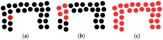
Figure 2. The handled geometry is colored red: (a) point level; (b) patch level; (c) object level.

At the point level (lowest level), the geometry is sparse and defines the lowest possible geometric description. While this is convenient for point-based rendering [108] that can be enhanced through deep learning [109], leading to simpler and more efficient algorithms [110], geometric clustering covers applications identified in Section 1. At the patch level, subsets of points are grouped to form small spatial conglomerates. These are better handled in a Point Cloud Database Management System (PC-DBMS) using a block-scheme approach which gives additional hints on the spatial context. At the object level, patches are grouped together to answer the underlying segmentation or classification approach. These three geometric levels are managed within the PC-DBMS module (Figure 3) and directly integrate semantics (segment, class, function, etc.) and space (abstract, geometric, etc.) information. While 3D modelling approaches solely based on spatial attributes can leverage both the SPC point and patch levels, using the additional information linked to the object level extend the range of shape representations, and thus applications.

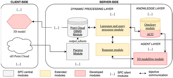
Figure 3. The Smart Point Cloud [29] tailored Infrastructure for 3D modelling.

Moreover, the SPC provides enough elasticity to centralize knowledge for decision-making scenarios. Its conception allows a mapping between domain specializations such as formalized IFC-inspired ontologies to provide additional reasoning possibilities. As a first step toward 3D point cloud modelling, and to permit knowledge-based reasoning for indoor applications, we tailored the SPC Server-Side Infrastructure as in Figure 3 with an applicative context ontology (ACO) for efficient KE, KI and KR.

In this infrastructure, we added a two-way mapping expert 3D modelling module (agent layer) to link 3D geometries to point data with semantic enrichment. The expert system consumes the SPC point cloud data with the ACO and will be further described in Section 3.2, Section 3.3 and Section 3.4.

To achieve semantic injection, we construct a multi-LoD IFC-inspired ontology (see Supplementary Materials). This provides knowledge about the object shapes, knowledge about the identities of objects and knowledge about the relationships between objects. Integrated into the knowledge layer (Figure 3) of the SPC, this ACO is used to best describe the morphological features of indoor elements in an interoperable manner. This new knowledge base is mainly used for refining the definition of objects within the SPC (Section 3.2), inferring modelling rules (Section 3.2) and providing clear guidelines for object-relationship modelling through the reasoner module (Section 3.4). For example, if the considered point cloud dataset benefits from additional information handled by the SPC such as the “space” definition, the reasoner will permit higher characterization (e.g., if the object is within an “office room”, there is a high chance that the chair is a “desk chair” with rolls). Moreover, the local topology available through the SPC provides additional information that is crucial regarding CSG-based modelling or for our object-relationship modelling approach (e.g., if a chair is topologically marked to be touching the floor, occlusion at its base can be treated accordingly).

With the aim of pooling our ontology in the Web of Linked Data, each object concept, if it exists, is defined as an extension of the DBpedia knowledge base. Providing such a link is an important interoperable feature when it comes to an object that is referred to as a DBpedia resource (e.g., for a chair object, http://dbpedia.org/page/Chair). The class hierarchy illustrated in Figure 4 is split into three main conceptual levels.

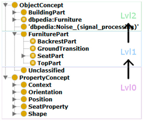
Figure 4. Class hierarchy in the ACO.

Level 0 is the first level of classified elements and defines properties established on point cloud features (shape, orientation, etc.). These features are stored in the knowledge base as datatype properties. Datatype properties are relations pointing from entities to literals (character strings, numbers, etc.). The values describe different bounding box characteristics: (length, width, etc.). Level 1 encapsulates Sub-Elements (SE) that are part of an Aggregated-Element (AE), defined in level 2. All entities that are not described within this hierarchy are categorized as “Unclassified”. Modelling rules at higher definition levels restrict the lower levels’ inferences through hierarchical constraints, similarly to [6]. These are strictly based on Sub-Elements, except for the topology relations between building parts and/or furniture. This consistency check permits the construction of complex definitions, but maintains a modularity for interoperability purposes. Semantic definitions of pre-labelled objects are extracted from the ACO ontology as depicted in Figure 5. Input variables are formed by labels of the retrieved object encapsulated in a JSON object part of the language processing module (Figure 3). Labels are then used to set SPARQL queries on a graph structure to query the ontology.

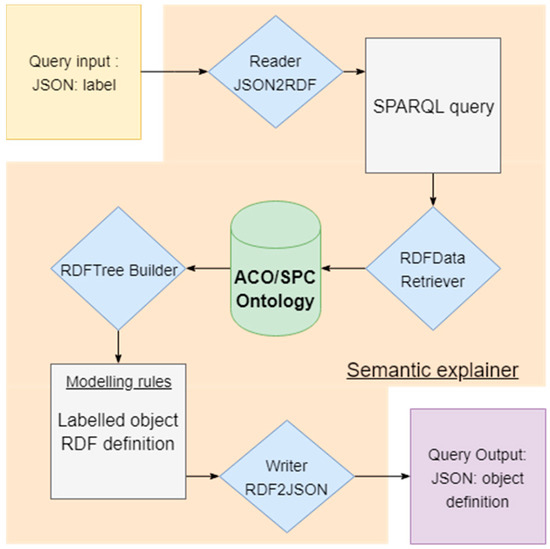
Figure 5. Framework for the extraction of an object definition from ACO to be readable by other modules of the SPC Infrastructure.

The ontology-based extraction of an object’s definition is the reverse-process of classification. It is thus possible to extract mandatory elements of objects for reconstruction and to guide their modelling. As each level is independent, reconstruction can be made at different LoD considerations. Graph-mining is guided by relation types between the elements of each level. E.g., a “chair” is composed of a chair back (BackrestPart) located somewhere above (this information is extracted from gravity-based topology analysis, as described in Section 3.2) a seat (oneSeat), with some ground transition parts (GroundTransitionPart) under it. Ontologies as XML-written files are well suited for hierarchical structures. A dedicated parser finally allows the answer to be structured in a JSON-file and communicated with the object characterization step (Section 3.2). Listing 1 shows the results of querying ACO/SPC Ontology about the “KitchenChair” label. It is structured as a hierarchical tree of characteristics, where each level is detailed by its sub-levels. In this tree, each line specifies a triple that refers to the object description (e.g., “hasNormale some PerpendicularOrientation” specifies that the normal needs to be perpendicular to the main orientation for this specific Sub-Element).

Listing 1 Kitchen Chair semantic definition extracted from the ACO

Label queried: “KitchenChair”

Detected element: http://www.geo.ulg.ac.be/nyspoux/SPC#KitchenChair hasPart min 4 http://www.geo.ulg.ac.be/nyspoux/SPC#GroundTransition hasNormale some PerpendicularOrientation hasIntersectionPerpendicular some http://www.geo.ulg.ac.be/nyspoux/SPC#FurniturePart hasAverageHistogram maxExclusive 0.25 hasContext some http://www.geo.ulg.ac.be/nyspoux/SPC#ContextKitchen hasPart some http://www.geo.ulg.ac.be/nyspoux/SPC#OneSeat hasWidth maxInclusive 0.45 hasThickness maxInclusive 0.45 hasLength maxInclusive 0.45 hasNormale some MainOrientation hasPart some http://www.geo.ulg.ac.be/nyspoux/SPC#BackrestPart hasNormale some PerpendicularOrientation hasIntersectionPerpendicular some http://www.geo.ulg.ac.be/nyspoux/SPC#SeatPart hasNormale some MainOrientation hasAverageHistogram minInclusive 0.75 hasFlatness maxExclusive 0.5 hasElongation minInclusive 0.5

The reasoning module depends on the language processing module (Figure 3). As the OWL formalism is a Description-Logic-based language, it allows logical consequence inferences from a set of stated axioms. We describe asserted facts in both the terminological box (TBox) and assertional box (ABox). TBox is constituted of class definitions in the ACO ontology, whereas individuals populate the ABox. Because of editing rules and restrictions on class definitions, those boxes are inferred and constitute our structure for knowledge discovery on logical reasoning. Listing 2 provides a simple example of inference based on both TBox and ABox. While TBox rules define the conditions for classifying an object as a Wall, ABox specifies that three objects exist. The first object is constituted by the two others as a collection, and these two subparts are defined as WallSurfaces.

Listing 2 Simple example of inferences on TBox and ABox

TBox rules and restrictions: :Wall owl:equivalentTo (hasPart min 2:WallSurface)

ABox population: :SubElement1 a:WallSurface :SubElement2 a:WallSurface :Object hasPart:Collection(:SubElement1 and:SubElement2)

Inferences: :Object a:Wall

Our approach was for indoor point clouds; thus, the ACO retains information for the following elements: beams, ceilings, floors, chairs, columns, doors, tables, walls and windows. These were primarily chosen due to existing workflows providing robust recognition. These elements are considered correctly categorized, and it is not necessary to filter point cloud artefacts. In Section 3.2, we present the second step (Figure 1B) of our workflow, which aims at generating modelling rules while retaining the specificity of each element.

3.2. Instance-Based Characterization, Feature Extraction and Description Refinement

While the SPC-integrated point cloud holds a minima class or segment information, these are not necessarily optimal with regard to indoor applications. The ACO makes it possible to deepen the classification of considered classes presented in Table 1 through the Web of Linked Data. For each class, every element is extracted independently from the point cloud and considered for instance characterization.

Table 1. Objects to be modelled from the S3-DIS point cloud dataset [111] are highlighted in red, identified by a major primitive (Cuboid, Plane, or CSG model assembly) and a category, being Normal-Element (NE), Sub-Element (SE) or Aggregated-Element (AE).

Beam	CeilingS	Chair	Column	Door	Table	WallS	Window
Cuboid	Plane	CSG model	Cuboid	CSG model	CSG model	Plane	Cuboid
NE	SE	AE	NE	AE	AE	SE	NE

Let $p_i$ be a point in ${ℝ}^s$, with $s$ the number of dimensions. We have a point cloud $\mathcal{P}={\left\{p_i\right\}}_{i=1}^n$ with $n$ the number of points in the point cloud. Let ${\mathcal{E}}_i$ be an element of $\mathcal{P}$ identified by a label ${\mathcal{L}}_i$, containing $m$ points from $\mathcal{P}$. Let $ℊ$ be a directed graph defined by a set $𝓋(ℊ)$ of inner nodes, a set $ℯ(ℊ)$ of edges and a set ${𝓋}_e(ℊ)$ of end nodes. Each edge is oriented regarding a specified topology relation between one or multiple nodes (its ends). Then, three processing cases arise from the definition of elements (Figure 6), where:

Figure 6. (a) ${\mathcal{E}}_i$ is a Normal-Element; (b) ${\mathcal{E}}_i$ is an Aggregated-Element, it goes through part-segmentation; (c) ${\mathcal{E}}_i$ is a Sub-Element.

(a)

${\mathcal{E}}_i$ is an element that is described in $ℊ$ as an end ${𝓋}_e(ℊ)$ (the final level of the elements decomposition, e.g., a wall, a beam, etc.). These elements are directly identified as Normal-Elements (NE) in the ACO Level 2 (Figure 4) and refer to a DBpedia resource. Such a case does not necessitate a part segmentation, and therefore allows the expert system to directly address the modelling phase (Section 3.3).

(b)

When ${\mathcal{E}}_i$ is an element described in $ℊ$ as a combination of multiple Sub-Elements (and therefore is in the category of Aggregated-Element from the SPC), it goes through part-segmentation (Section 3.2) before modelling the entity. This segmentation is guided by inferred rules extracted from the ACO ontology. For instance, if an object is labelled as a “kitchen chair”, its definition will specify that segmentation need to find an upper-part, which is a backrest, a middle-part, which is a oneSeat, and some ground transition parts—at least 3 for the example of the “kitchen chair”.

(c)

When ${\mathcal{E}}_i$ is a Sub-Element in the ACO and refers to an Aggregated-Element, the point cloud subset goes through an aggregation step before modelling. This step is guided by semantic definitions and symmetric operations to find (recreate) other Sub-Elements of the Aggregated-Element. For instance, when a WallSurface is considered to be ${\mathcal{E}}_i$, its parallel wall surface will be searched for in the SPC database to constitute the Aggregated-Element “Wall”.

The main processes of this second step are described in Algorithm 1 as part of the global workflow.

Algorithm 1 Element characterization, featuring and generation of modelling rules (Figure 1B)

Require: A point cloud $\mathcal{P}\in {ℝ}^s,$ decomposed in n ${\mathcal{E}}_i$ each with a label ${\mathcal{L}}_i$

For each ${\mathcal{E}}_i$ do  ${\mathrm{C}}_{{\mathcal{E}}_i}\leftarrow$ characterization of ${\mathcal{E}}_i$ (NE, SE or AE)  if ${\mathrm{C}}_{{\mathcal{E}}_i}==‘AE’$ then  specialization of ${\mathcal{E}}_i$ through part-segmentation  end if  ${\mathcal{E}}_i{}^{+}\leftarrow$ Add Bag of features, Object relationship information and Contextual semantics  $\mathcal{R}\leftarrow$ Generation of modelling rules through ACO  end for  end  return (${\mathcal{E}}_i{}^{+},\mathcal{R}$)

While NE and SE’s characterization avoids part-segmentation, AE goes through case (b) for a higher representativity. Looking at the considered AE classes (chair, door, table), the “chair” class provides the highest variability for testing and will thus be used as the main illustration of AE specialization and shape featuring (Figure 1B). We decompose this mechanism (Algorithm 1: line 4) into three sub-steps.

Sub-Step 1. Pose determination of 3D shapes: we use a robust variant of Principal Component Analysis (PCA) inspired by Liu and Ramani [76], to compute the principal axis of points composing ${\mathcal{E}}_i$ (Algorithm 2). The eigen vector with the largest value in the covariance matrix is chosen as the first estimate of the principal direction.

Algorithm 2 Robust Principal Axis Determination (RPAD)

Require: A point cloud object ${\mathcal{E}}_i\in {ℝ}^3$ filtered for considering only spatial attributes along $\overrightarrow{x},\overrightarrow{y},\overrightarrow{z}$, $\max \_iteration$ the maximum number of iteration (by default: 1000),

$𝓅\leftarrow$ inliers candidates from Statistical Outlier Identification Filter [112] applied to ${\mathcal{E}}_i$  while $j<\max \_iteration$ do  $ℴ,\overrightarrow{e_1},\overrightarrow{e_2},\overrightarrow{e_3}\leftarrow$ origin and three principal axes of $𝓅$ through PCA  $r\leftarrow {\mathcal{E}}_i-𝓅$, remaining points as a matrix in ${ℝ}^3$, $r_i$ being a point $p_i\in r$  $res(r_i)\leftarrow$ the distance between $r_i$ and its projection onto $\overrightarrow{e_1}$  if $\left|res(r_i)\right|<\left|mean(res)+\sigma \right|$ then  $𝓅.append(r_i)$  end if  end while  $\overrightarrow{e_2},\overrightarrow{e_3}\leftarrow$ Update by a 2D RPAD over ${\mathcal{E}}_i$ projection onto the plane defined by $\overrightarrow{e_2},\overrightarrow{e_3}$  end  return ($ℴ,\overrightarrow{e_1},\overrightarrow{e_2},\overrightarrow{e_3}$)

We provide an additional refinement layer leveraging georeferenced datasets and gravity-based scenes by constraining the orientation of Sub-Elements (Algorithm 3):

Algorithm 3 Gravity-based constraints for Sub-Elements ${\mathcal{E}}_{sub-i}$

Require: A point cloud Sub-Element ${\mathcal{E}}_{sub-i}\in {ℝ}^3$ and $ℴ,\overrightarrow{e_1},\overrightarrow{e_2},\overrightarrow{e_3}$, the output of Algorithm 2

${ℴ}_s,\overrightarrow{s_1},\overrightarrow{s_2},\overrightarrow{s_3}\leftarrow$ origin and three principal axes of ${\mathcal{E}}_{sub-i}$ through RPAD  $\overrightarrow{p_{\overrightarrow{s1}}}\leftarrow$ projection of the main axis $\overrightarrow{s_1}$ onto the plane defined by the normal $\overrightarrow{e_3}$ from $mainElement({\mathcal{E}}_i)$ as defined in ACO  ${\alpha }_1, {\alpha }_2\leftarrow$ angle respectively $\widehat{(\overrightarrow{e_1,}\overrightarrow{p_{\overrightarrow{s1}}})}$ and $\widehat{(\overrightarrow{e_2,}\overrightarrow{p_{\overrightarrow{s1}}})}$  if ${\alpha }_1\le {\alpha }_2$ then  $\overrightarrow{s_2}\leftarrow R_z({\alpha }_1)\overrightarrow{s_2}$ and $\overrightarrow{s_3}=\overrightarrow{s_1}\times \overrightarrow{s_2}$  elif: $\overrightarrow{s_2}\leftarrow R_z({\alpha }_2)\overrightarrow{s_2}$  end  return (${ℴ}_s,\overrightarrow{s_1},\overrightarrow{s_2},\overrightarrow{s_3}$)

Sub-Step 2. The 2nd sub-step in the part-segmentation process extracts several shape features which guide the process. Every point $p_i$ composing ${\mathcal{E}}_i$ is processed following Algorithm 4:

Algorithm 4 Histogram and bin featuring of an element ${\mathcal{E}}_i$

Require: A point cloud object ${\mathcal{E}}_i\in {ℝ}^3$ filtered for considering only spatial attributes $X,Y,Z$ along $(\overrightarrow{x},\overrightarrow{y},\overrightarrow{z})$ axis, $X_e,Y_e,Z_e$ the spatial attributes along principal directions $(\overrightarrow{e_1},\overrightarrow{e_2},\overrightarrow{e_3})$

$\mathcal{B}\leftarrow$ bin gridded elementary subset of ${\mathcal{E}}_i$, by default an octree-based voxel [33]  $done\leftarrow \varnothing$  for each $\mathcal{B}$ do  if $\mathcal{B}.index$ is not in $done$ then  $done\leftarrow$ $done.append(\mathcal{B}.index)$  ${\mathrm{C}}_{\mathcal{B}} \leftarrow$ Coordinates $(X_{\mathcal{B}c},Y_{\mathcal{B}c},Z_{\mathcal{B}c})$ of the center of $\mathcal{B}$ as a vector in ${ℝ}^3$  ${\mathcal{F}}_{(\overrightarrow{e_2},\overrightarrow{e_3})}\leftarrow$ count number of bin $\mathcal{B}$ with same $(Y_{\mathcal{B}c},Z_{\mathcal{B}c})$ along $\overrightarrow{e_2},\overrightarrow{e_3}$, and different $X_{\mathcal{B}c}$ along $\overrightarrow{e_1}$  ${\mathcal{F}}_{\overrightarrow{e_1}}\leftarrow$ count number of bin $\mathcal{B}$ with same $X_{\mathcal{B}c}$ along $\overrightarrow{e_1}$, and different $(Y_{\mathcal{B}c},Z_{\mathcal{B}c})$ along $\overrightarrow{e_2},\overrightarrow{e_3}$  end if  end for  end  return (${\mathcal{F}}_{(\overrightarrow{e_2},\overrightarrow{e_3})},{\mathcal{F}}_{\overrightarrow{e_1}}$) as a dictionary with the ${\mathrm{C}}_{\mathcal{B}}$ as a key, and ${\mathcal{F}}_{(\overrightarrow{e_2},\overrightarrow{e_3})},{\mathcal{F}}_{\overrightarrow{e_1}}$ as values

Outputs of Algorithm 4 are used as initial shape descriptors for studying local maxima. This is done through a gradient approach with different neighborhoods to avoid over/under segmentation. The gradient $\overrightarrow{\nabla }(f)$ is computed using central difference in the interior and first differences at the boundaries:

$$\overrightarrow{\nabla }(f)=\frac{\delta f}{\delta x}\overrightarrow{i}+\frac{\delta f}{\delta y}\overrightarrow{j}$$

(1)

$${\delta }_h\left[f\right](x)=f(x+\frac{1}{2}h)-f(x-\frac{1}{2}h),\mathrm{with}h=1(\mathrm{interior})$$

(2)

$${\Delta }_h\left[f\right](x)=f(x+h)-f(x)(\mathrm{boundaries})$$

(3)

From the extrema, we descend the gradient to find the two cut candidates: downcut and upcut. This is iteratively refined by studying each extremum and their relative cuts. When two extrema have a common value for their cuts, they are studied for possible under segmentation, and therefore aggregated into the initial candidate. Cut candidates are extracted by fitting a linear least-square model to each gradient after extrema’s filtering to identify the baseline (Figure 7: line 5). This makes it possible to be robust to varying sampling distances, missing point cloud data and outliers. We then extract the candidate for the Main-Element, and we further process Sub-Elements.

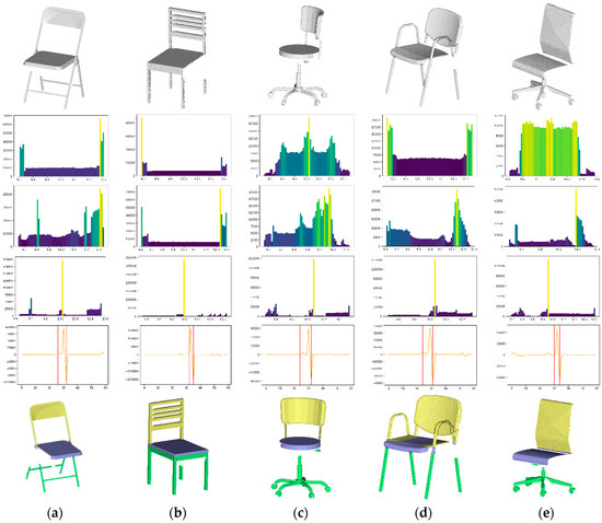
Figure 7. Each AE from (a–e) is projected in a voxelized space, studied against voxel count per unit over $\overrightarrow{e_1},\overrightarrow{e_2},\overrightarrow{e_3}$ to extract extrema and find patterns that define each Sub-Element in the ACO. For each object, line 1 is the considered AE, line 2 to 4 illustrates the repartition histogram along $\overrightarrow{e_1},\overrightarrow{e_2},\overrightarrow{e_3}$, line 5 the principal cuts extracted, line 6 the results.

Sub-Step 3. The ontology contains a knowledge-based symmetry indicator which provides insights on the possible symmetric properties of each class, expressed regarding the Main-Element (see Supplementary Materials). We first use these, and if the test fails, we undertake a specific symmetry search using analytic knowledge, similarly to [86]. In the context of indoor point clouds, we mostly deal with approximate symmetries due to measured data. Therefore, we use a measure of overlap by mapping the pixels as binary grid of the projection on a plane the normal of which is coplanar to the symmetry plane and vice-versa (Figure 8: line 2). The symmetry analysis is conducted over the repartition histogram projected onto the plane $(\overrightarrow{e_2},\overrightarrow{e_3})$. Then we run mean-shift clustering to detect candidate axis positions among all pairs of neighboring patches, similarly to [87].

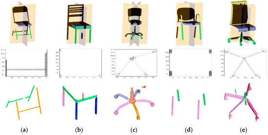
Figure 8. Symmetric feature characterization for Sub-Elements of chairs (a–e). Line 1: symmetric planes; line 2: 2D projection features; line 3: similarity feature tag results for other Sub-Elements.

At this point, we benefit from a better characterization of AE through the ACO and the described threefold mechanism. Each initial element composing the scene (NE, SE and AE) is then processed to extract object relationships. We construct a connected component graph $ℊ$ in a voxel-space based on the initial bounding-box parameters of $\mathcal{P}$ and the one of the considered element ${\mathcal{E}}_a$. We then use the available topology information ${\mathcal{T}}_v(v_a,{\left\{v_i\right\}}_{i=1}^{26})$, computed with regard to DE-9IM [113] in the voxel space and extended using spatial operators, to identify elements related to ${\mathcal{E}}_i$ along $\overrightarrow{e_1}$:

$$relation=\left\{guest,host,twin\right\},$$

(4)

$$\forall i \in relation, \exists ({\mathcal{E}}_a,{\mathcal{E}}_b) | \mathcal{T}({\mathcal{E}}_a,{\mathcal{E}}_b)=i,$$

(5)

$$ℯ(ℊ)= \mathcal{T}({\mathcal{E}}_a,{\mathcal{E}}_b) with {\mathcal{E}}_a=𝓋(ℊ), {\mathcal{E}}_b={𝓋}_e(ℊ)$$

(6)

The basic object relationship is defined as $\mathcal{T}({\mathcal{E}}_a,{\mathcal{E}}_b)$ and determined using Algorithm 5:

Algorithm 5 Object-relationship definition for indoor elements

Require: A point cloud object ${\mathcal{E}}_i\in {ℝ}^3$ filtered for considering only spatial attributes $X,Y,Z$ along $(\overrightarrow{x},\overrightarrow{y},\overrightarrow{z})$ axis, ($\overrightarrow{e_1},\overrightarrow{e_2},\overrightarrow{e_3}$) the principal directions, $X_e,Y_e,Z_e$ the spatial attributes along $\overrightarrow{e_1},\overrightarrow{e_2},\overrightarrow{e_3}$

${\mathcal{T}}_v(v_a,{\left\{v_i\right\}}_{i=1}^{26})\leftarrow$ SPC voxel-based feature for direct voxel topology between $\mathcal{E}$  for each $\mathcal{E}$ do  if ${\mathcal{T}}_v(v_a,{\left\{v_i\right\}}_{i=1}^{26})=true$ and $v_i \in {\mathcal{E}}_b$ then  if ${\max }_{\overrightarrow{e_1}}(BBox({\mathcal{E}}_b))<{\min }_{\overrightarrow{e_1}}(BBox({\mathcal{E}}_a)) \mathbf{and} |{\min }_{\overrightarrow{e_1}}(BBox({\mathcal{E}}_a))-{\max }_{\overrightarrow{e_1}}(BBox({\mathcal{E}}_b))|<K{B}_{th}$ then  $\mathcal{T}({\mathcal{E}}_a,{\mathcal{E}}_b)=guest$  elif $\mathcal{T}({\mathcal{E}}_b,{\mathcal{E}}_a)=guest$ then $\mathcal{T}({\mathcal{E}}_a,{\mathcal{E}}_b)=host$  elif ($\mathcal{T}({\mathcal{E}}_a,{\mathcal{E}}_b)=guest$ or $\mathcal{T}({\mathcal{E}}_a,{\mathcal{E}}_b)=host$) and $\left|X_{\overrightarrow{e_1}}(CenterBBox({\mathcal{E}}_a))-X_{\overrightarrow{e_1}}(CenterBBox({\mathcal{E}}_b))\right|<K{B}_{th}$ then $\mathcal{T}({\mathcal{E}}_a,{\mathcal{E}}_b)=twin$  end if  end if  end for  end  return ($\mathcal{T}({\mathcal{E}}_a,{\mathcal{E}}_b)$) for every $\mathcal{E}$ composing $\mathcal{P}$

With regard to AE, Sub-Elements that create new segments are similarly refined, using the ACO (e.g., if ${\mathcal{E}}_i$ is a “Kitchen Chair” and the number of ${\mathcal{E}}_{sub-i}$ in “someDown” position is lower than 3, then the results are refined, as a “Kitchen Chair” is described having at least 3 legs). Guided by ACO, we cross-relate ${\mathcal{E}}_i$ information $\mathcal{F}\ell$, $\mathcal{W}\mathcal{𝒾}$, $\mathcal{L}e$, ${\mathcal{F}}_{(\overrightarrow{e_2},\overrightarrow{e_3})}, {\mathcal{F}}_{\overrightarrow{e_1}}$, $\mathcal{H}ℯ$ and $\mathcal{E}\ell$ with the highest maximas, where:

$$\forall X_e<Y_e, \exists \mathcal{L}e\in ℝ | \mathcal{L}e=Y_e, \forall X_e>Y_e, \exists \mathcal{L}e\in ℝ | \mathcal{L}e=X_e$$

(7)

$$\mathcal{W}𝒾=\min (\overrightarrow{e_1},\overrightarrow{e_2}), \mathcal{T}𝒽=Z_e, \mathcal{F}\ell =\frac{\mathcal{T}𝒽}{\mathcal{W}𝒾}, \mathcal{E}\ell =\frac{\mathcal{W}𝒾}{\mathcal{L}e}$$

(8)

These are grouped as a bag of features and we infer modelling rules (e.g., Figure 9) after going through a language processing step to provide three groups of features:

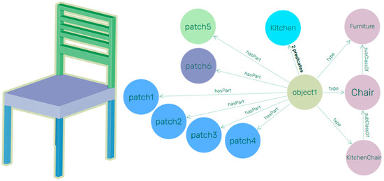
Figure 9. The ACO graph representation of the chair and the relations within Sub-Elements.

-

Bag of features: Flatness $\mathcal{F}\ell$, Width $\mathcal{W}𝒾$, Length $\mathcal{L}e$, Histogram features (${\mathcal{F}}_{(\overrightarrow{e_2},\overrightarrow{e_3})}, {\mathcal{F}}_{\overrightarrow{e_1}}$), Height $\mathcal{H}ℯ$, Elongation $\mathcal{E}\ell$, Thickness $\mathcal{T}𝒽$, Main orientation $\overrightarrow{e_1}$.

-

Object-relationship information: Topology relation $\mathcal{T}({\mathcal{E}}_a,{\mathcal{E}}_b)$, Relative position to elements in fixed radius $\mathcal{R}({\mathcal{E}}_a,{\mathcal{E}}_b)$, Direct voxel-based Topology ${\mathcal{T}}_v(v_a,{\left\{v_i\right\}}_{i=1}^{26})$

-

Contextual semantics: Semantic position ${\mathcal{R}}_s({\mathcal{E}}_a,\mathcal{P})$, Function ${\mathcal{F}}_i$, Label ${\mathcal{L}}_i$

Contrary to [6], we do not reason based on decision trees that are extracted from an ontology. Indeed, we create a JSON object per element ${\mathcal{E}}_i$ that holds the Bag of features, Object-relationship information and Contextual semantics. These include concepts of physics and causation such as stability, clearance, proximity and dimensions defined as Knowledge Primitives by Sutton et al. [114]. The reasoning module of the expert system can in turn provide the guiding modelling rules $\mathcal{R}$ for the considered object as developed in Section 3.1.

In the next sub-section (Figure 1C) we explain the third step of our global workflow, which provides a modelling approach for obtaining multiple geometries for each ${\mathcal{E}}_i$ composing $\mathcal{P}$.

3.3. Procedural Instance 3D Modelling

As reviewed in Section 2.1, most indoor scenes are primitive-based decompositions. As such, we provide a simple yet efficient parametric instance-modelling, described in Algorithm 6, that reconstructs each element ${\mathcal{E}}_i$ using cuboid and bounded plane representations.

Algorithm 6 Multi-LoD object instance modelling (Figure 1C)

Require: Algorithm 1 output: $({\mathcal{E}}_i{}^{+},\mathcal{R})$

For each ${\mathcal{E}}_i{}^{+}$ do  if ${\mathrm{C}}_{{\mathcal{E}}_i{}^{+}}==‘AE’$ then  ${\mathcal{E}}_i{}^{+}$ goes through part-modelling and part-assemblage  end if  ${\mathcal{E}}_i{}^{+}$ parameters refinement through context adaptation following $\mathcal{R}$ specifications  {${\mathcal{M}}_{L0},{\mathcal{M}}_{L1},{\mathcal{M}}_{L2},{\mathcal{M}}_{L3}\}\leftarrow$ Primitive fitting for multi-LoD 3D model generation  ${\mathcal{M}}_{3DM}\leftarrow$ Model from 3D Data mining using ModelNet10 based on $\{{\mathcal{M}}_{L0},{\mathcal{M}}_{L1},{\mathcal{M}}_{L2}\}$  end for  end  return (${\mathcal{M}}_{L0},{\mathcal{M}}_{L1},{\mathcal{M}}_{L2},{\mathcal{M}}_{L3},{\mathcal{M}}_{3DM}$)

Similar to Step 2 (Figure 1B, Section 3.2) of the global workflow, the characterization of the AE element as ${\mathcal{E}}_i{}^{+}$ is accounted for by going through a specific part-modelling and part-assemblage processing (necessitate AE’s characterization and part-segmentation, as detailed in Section 3.2). This is done by considering each Sub-Element of the initial element ${\mathcal{E}}_i$ an independent element. Then, using intra-${\mathcal{E}}_i$ topology (relations between Sub-Elements from part-segmentation) defined within the ACO, geometric parameters are adjusted (Figure 10).

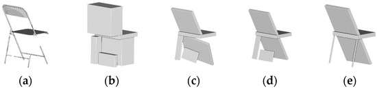
Figure 10. The different phases of the primitive fitting for AE. (a) Point cloud; (b) Raw parameters and generation of grid-aligned cuboid; (c) Refinement by non-constrained PCA-Analysis; (d) Refinement by constrained PCA-Analysis; (e) parameters refinement through ACO.

The parametrization of generated models gives users the ability to alter the entire logic of the object construction by adjusting individual parts.

We parametrize a cuboid with three orthogonal directions $\overrightarrow{c_1},\overrightarrow{c_2},\overrightarrow{c_3}$ where:

$$\overrightarrow{c_3}=\overrightarrow{c_1}\times \overrightarrow{c_2}$$

(9)

The cuboid parameters also include the center coordinates $X_c,Y_c,Z_c$, as well as the length, width and height, respectively, along $\overrightarrow{c_1},\overrightarrow{c_2},\overrightarrow{c_3}$. Its finite point set representation is obtained by tessellation and generated as an obj file. A bounded plane is represented by a set of parameters $p=\left\{p_1,p_2,p_3,p_4\right\}$ that defines a plane, and a set of edge points $e$ that lies in the plane and describes the vertices of the plane’s boundary.

Depending on ${\mathcal{E}}_i$’s characterization, we obtain a geometric model composed of a bounded plane, a cuboid, a cuboid assembly or a cuboid and bounded plane aggregation. These geometries are then refined to provide multiple LoD. ${\mathcal{E}}_i$ are found represented as Bounding-box (${\mathcal{M}}_{L0}$), Trivial knowledge-based parametric shape (${\mathcal{M}}_{L1}$), Parametric assemblage (${\mathcal{M}}_{L2}$) and hybrid voxel-based refined model (${\mathcal{M}}_{L3})$, as illustrated in Figure 11 and executed in Algorithm 6: line 6.

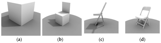
Figure 11. (a) Bouding-box ${\mathcal{M}}_{L0}$; (b) KB model ${\mathcal{M}}_{L1}$; (c) Assemblage ${\mathcal{M}}_{L2}$; (d) hybrid model ${\mathcal{M}}_{L3}$.

As an alternative to the 3D models extracted from the procedural engine, we study a 3D database shape matching approach for higher geometric flexibility, but also to provide a way to extract additional information from external database sources through mining. We consider database objects from the ModelNet10 [35] library, specifically the chair, desk and table furniture due to the non-availability of wall, beam, ceiling and floor models (Figure 12). Each candidate is oriented in the same way (Main-Element’s $\overrightarrow{e_3}$ is $\overrightarrow{z}$-aligned, $\overrightarrow{e_2}$ is $\overrightarrow{y}$-aligned), which makes it possible to avoid global alignment search and local refinement via ICP. Only a rigid translation and deformable step is executed. The main challenges include the present noise in scanned data, isotropic shapes, partial views and outliers. As such, global matching methods based on exhaustive search (efficient if we can strongly constrain the space of possible transformations), normalization (not applicable to partial views, or scenes with outliers) and RANSAC (need at least 3 pairs of points) are limited. We investigate an invariance-based method to try and characterize the shapes using properties that are invariant under the desired transformations. We describe each database 3D model by computing a rank $R_{Level-1}$ to define a first set of best fit candidates $C_i$, where:

$$R_{Level-1}(C_i)=\left|\frac{\mathcal{H}ℯ({\mathcal{M}}_{L1})}{\mathcal{L}e({\mathcal{M}}_{L1})}-\frac{\mathcal{H}ℯ(C_i)}{\mathcal{L}e(C_i)}\right|+\left|\frac{\mathcal{H}ℯ({\mathcal{M}}_{L1})}{\mathcal{W}𝒾({\mathcal{M}}_{L1})}-\frac{\mathcal{H}ℯ(C_i)}{\mathcal{W}𝒾(C_i)}\right|$$

(10)

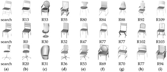
Figure 12. Results of the shape matching over different datasets (a). The rank RXX represents the score of each candidate. The closer to 0, the better the shape fits the search from (b–i).

We then compare each rank for each candidate within the database and filter by score. We narrow the set of candidates by comparing its symmetry pointer to ${\mathcal{E}}_i{}^{+}$ and each Sub-Element (when applicable), which highly constrains the repartition. This is done regarding the symmetry descriptors as defined in Section 3.2. The new rank descriptor $R_{Level-2}$ is given by:

$$R_{Level-2}(C_i)=R(similarit{y}_{ratio})+R_{Level-1}(C_i)$$

(11)

We compute the transformation parameters by matching the centroids of $C_i$ and ${\mathcal{M}}_{L1}$, refined using ${\mathcal{M}}_{L2}$ and ACO-inferred ${\mathcal{E}}_i{}^{+}$ for its orientation. We finally adjust scale by matching shape parameters. This is done using the symmetry indicators and planes as coplanar constraints for global transformation with independent shape deformation along each principal axis.

Finally, in the next section we present the closing step in aggregating every modelled element to create a 3D model accompanied by object relationships (Figure 1D, Section 3.4).

3.4. 3D Aggregation for Scene Modelling

At this stage, every element ${\mathcal{E}}_i$ composing $\mathcal{P}$ is enhanced to retain contextual information and object-relationship through Algorithm 1, becoming ${\mathcal{E}}_i{}^{+}$. It is then processed in accordance with $\mathcal{R}$ from the ACO to obtain a set of models {${\mathcal{M}}_{L0},{\mathcal{M}}_{L1},{\mathcal{M}}_{L2},{\mathcal{M}}_{L3},{\mathcal{M}}_{3DM}$} using Algorithm 6. The final step (Figure 1D) is to leverage the context with related elements for general modelling, with adjusted parametric reconstruction, notably following the topology and symmetric considerations. E.g., the constraints extracted by processing the ACO—such as “the feet have the same height”, derived from topological reasoning with the ground—permit contextual inference. Every element is then aggregated as described in Algorithm 7, and object-relationships ${\mathcal{R}}_{G3D}$ are retained to be usable concurrently with the global 3D indoor model ${\mathcal{M}}_{G3D}$. This step follows a part-to-whole design which starts with the floors, ceilings, walls, beams/columns and then goes to doors, windows then furniture.

Algorithm 7 Element aggregation for global geometric and relationship modelling (Figure 1D)

Require: Algorithm 1 output $({\mathcal{E}}_i{}^{+},\mathcal{R})$ and Algorithm 6 output (${\mathcal{M}}_{L0},{\mathcal{M}}_{L1},{\mathcal{M}}_{L2},{\mathcal{M}}_{L3},{\mathcal{M}}_{3DM})$

${\mathcal{M}}_{G3D}\leftarrow \varnothing$  For every ${\mathcal{E}}_i{}^{+}\in \mathcal{P}$ do  if ${\mathcal{L}}_i \ne door$ or ${\mathcal{L}}_i \ne window$ then  ${\mathcal{M}}_{G3D}\leftarrow$ ${\mathcal{M}}_{G3D}\cup {\mathcal{M}}_{Xi}$: Aggregate desired ${\mathcal{E}}_i$ geometry (${\mathcal{M}}_{Xi})$ from the set of models {${\mathcal{M}}_{L0},{\mathcal{M}}_{L1},{\mathcal{M}}_{L2},{\mathcal{M}}_{L3},{\mathcal{M}}_{3DM}$} for natural or hybrid models  elif: ${\mathcal{M}}_{G3D}\leftarrow {({\mathcal{M}}_{G3D}\cap {\mathcal{M}}_{Xi})}^C+{\mathcal{M}}_{Xi}\cap {({\mathcal{M}}_{G3D}\cap {\mathcal{M}}_{Xi})}^C$  end if  ${\mathcal{R}}_{G3D}\leftarrow$ Object Relationship modelling of ${\mathcal{M}}_{G3D}$  end for  end  return (${\mathcal{M}}_{G3D},{\mathcal{R}}_{G3D}$)

To be topologically consistent in the sense of 3D modelling, we treat overlapping similarly to Fayolle and Pasko [51]. We represent a constructive model using a binary (CSG) construction tree structure with primitive solids at the leaves and operations at the internal nodes of the tree. For any given point in space, an evaluation procedure traverses the tree and evaluates membership predicates at this point. After evaluation, we obtain a consistent 3D model of the entire scene retaining object-relationships. We use the Union (U) and Intersection (∩) operators and their set complements to refine the CSG-tree for modelling the point cloud (Figure 13).

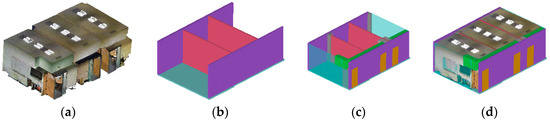
Figure 13. (a) S3-DIS Point Cloud extract; (b) SE modelling (walls, floors, ceilings); (c) NE completion and CSG operations; (d) 3D global model with point cloud superimposition.

The ability to use several representations from the set of instance models {${\mathcal{M}}_{L0},{\mathcal{M}}_{L1},{\mathcal{M}}_{L2},{\mathcal{M}}_{L3},{\mathcal{M}}_{3DM}$} makes it possible to obtain hybrid models following the same mechanism as illustrated in Figure 14.

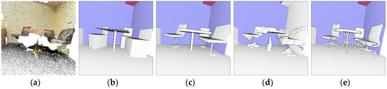
Figure 14. (a) S3-DIS; (b) (${\mathcal{M}}_{L0},{\mathcal{M}}_{L1}$) model; (c) (${\mathcal{M}}_{L0},{\mathcal{M}}_{L2}$ ) model; (d) (${\mathcal{M}}_{L0},{\mathcal{M}}_{L3}$ ) model; (e) (${\mathcal{M}}_{L1},{\mathcal{M}}_{3DM}$ ) model.

With the aim of aggregating semantics outside the SPC Infrastructure and for interoperability with existing standards, we obtain a parsing-ready JSON object for IFC file construction. ${\mathcal{M}}_{L0},{\mathcal{M}}_{L1},{\mathcal{M}}_{L2},{\mathcal{M}}_{L3}$ and ${\mathcal{M}}_{3DM}$ geometries follow the obj physical file format to be mapped in the IFC scheme using the EXPRESS data definition language. For beams, floors, and walls, IFC entity types, such as IfcBeam, IfcWall, IfcWallStandardCase, IfcBulidingElementProxy, IfcRelDecomposes and IfcRelConnects, are defined with their geometric and connectivity properties following the IFC scheme. In this way, an as-built 3D model of the structural elements compliant with industry standards can be inferred.

4. Results

In this section, we detail the results of our methodology through several comparisons. We start by describing the underlying datasets, we then present the results of our evaluations to finally provide the details of our implementation and computation time. Then we provide identified limitations and research directions.

4.1. Datasets

The methodology was tested over three different datasets. The first dataset (SIM) is simulated data using the ModelNet10 library as scanning environment. The second (DAT) contains real data from actual sites using both the Leica P30 and Trimble TX5 terrestrial laser scanner. The last dataset is the S3-DIS created using the Matterport. The main idea behind using these various datasets is to use the simulated one to test the theoretical basis of the proposed approach, while the real datasets cover the difficulties and the efficiency of the method. The two real-world scenes (DAT and S3-DIS) represent indoor built environments. For the simulated cases (SIM), the point cloud was generated by 3D mesh tessellation and then by adding 2 mm of noise, which is representative of many current laser scanners. Subsampling is not employed at any stage, here, both for point clouds and 3D models. The simulated dataset is solely comprised of furniture (chair, desk, table), with around 1 million points per element. The DAT dataset is comprised of 800 million points, whereas the S3-DIS dataset contains over 335 million points, with an average of 55 million points per area (6 areas). The DAT presents many large planar surfaces and has a high device accuracy, resulting in low noise and a homogeneous point repartition. In contrast, the S3-DIS dataset is very noisy and presents many occluded areas. As these are typical scenes from the built environment, it is worth noting that they all present some significant levels of symmetry and/or self-similarity. Moreover, the DAT and 3D-DIS rely on a scan acquisition methodology that does not cover the full environment, presenting many occluded areas.

4.2. Comparisons

We tested our approach on both simulated and real-world point clouds of indoor buildings. We first provide in Table 2 the results of the part-segmentation for AE characterization (Section 3.2).

Table 2. Results of the part-segmentation mechanism against manually annotated Sub-Elements. The precision and recall were obtained by studying True Positives, False Positives and False Negatives ($\mathit{precision}=\frac{\mathit{True}\mathit{Positive}}{\mathit{True}\mathit{Positive}+\mathit{False}\mathit{Positive}},\mathit{recall}=\frac{\mathit{True}\mathit{Positive}}{\mathit{True}\mathit{Positive}+\mathit{False}\mathit{Negative}}$).

Dataset	Element	Legs		OneSeat		BackRest
		precision	recall	precision	recall	precision	recall
	chair_0001	99.99%	97.34%	93.52%	99.62%	99.99%	96.87%
	chair_0007	59.18%	99.99%	99.99%	87.22%	99.99%	99.99%
SIM	chair_0008	99.99%	99.99%	98.60%	99.99%	99.99%	98.56%
	chair_0029	99.99%	90.93%	95.82%	99.72%	99.99%	99.99%
	chair_0041	99.99%	99.99%	96.68%	99.99%	99.99%	97.31%
	overall	91.84%	97.65%	96.92%	97.37%	99.99%	98.55%
	F1-score	94.66%		97.14%		99.27%
		precision	recall	precision	recall	precision	recall
	chair_0001	99.99%	99.90%	98.32%	99.99%	99.99%	99.29%
	chair_0002	99.99%	93.57%	93.59%	83.68%	92.09%	98.97%
	chair_0005	99.99%	99.99%	99.99%	38.36%	29.70%	99.99%
DAT	chair_0006	96.14%	99.99%	87.29%	99.56%	95.02%	96.50%
	chair_0007	96.60%	99.99%	92.35%	88.25%	83.89%	98.79%
	overall	98.55%	98.69%	94.31%	81.97%	80.14%	98.71%
	F1-score	98.62%		87.71%		88.46%
		precision	recall	precision	recall	precision	recall
	chair_0001	99.99%	99.99%	89.26%	99.99%	99.99%	87.56%
	chair_0002	87.53%	99.99%	80.76%	73.31%	94.98%	91.85%
	chair_0003	99.99%	99.99%	97.51%	99.99%	99.99%	97.54%
S3-DIS	chair_0004	99.99%	99.99%	90.88%	99.99%	99.99%	92.13%
	chair_0005	99.99%	99.99%	90.55%	72.25%	74.94%	92.66%
	overall	97.51%	99.99%	89.79%	89.11%	93.98%	92.35%
	F1-score	98.74%		89.45%		93.16%

Firstly, we notice an overall precision and recall score above 90% for every Sub-Element of the SIM dataset. While the backRest gives the higher F1-score (99.27%), the oneSeat and the legs achieve lower scores of 97.14% and 94.66%, respectively. Indeed, these Sub-Elements are more subject to missing data which induce False Negatives. Specifically, the SIM chair_0007 represents a problematic case in which the point distribution’s features impact the segmentation through a high number of True Negatives. This can be solved if we include a connectivity step to merge similar Connected Components by looking at their Bag of features and their voxel topology. As for the recall indices, the problematic zones are often localized at the joints between each Sub-Element, which could be further refined if an additional (time-consuming) nearest neighbor search was implemented. Logically, the non-simulated datasets DAT and S3-DIS achieve lower scores for the backRest and oneSeat robustness detection. Recall drops by 7.43%, on average, and precision by 8.90%. This is specifically due to the non-uniform sampling of real-world datasets which present many occluded areas for these Sub-Elements, inducing many False Positives. Interestingly, we note that both DAT and S3-DIS datasets present an increase of around 4% for the F1-score. Indeed, the low precision and scan angle play in favor of joint identification between the oneSeat and the legs, which in turn increase the segmentation accuracy. We could highlight that the quality and robustness of our AE’s characterization approach depends on the plane detection quality, which is influenced by scanner noise, point density, registration accuracy, and clutter inside of the building.

Secondly, we assess the different LoD models obtained following Section 3.3. As the modelling approach does not aim at a perfect fitting of the underlying point cloud, we used an RMSE indicator for comparison between the model and the different reconstructions (Figure 15). We also compared the different sizes of generated geometries to obtain ratios of precision over complexity.

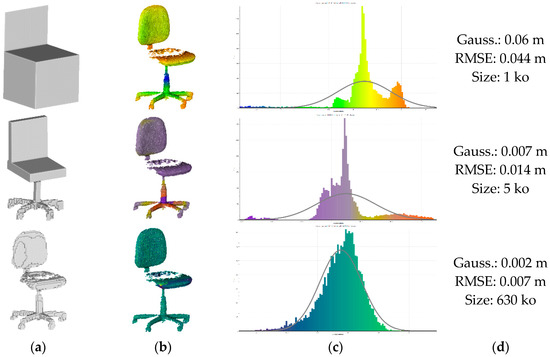
Figure 15. 3D modelling results over $\mathcal{M}L1,\mathcal{M}L2,\mathcal{M}L3$ of the DAT dataset. (a) 3D representation; (b) color-coded deviations from (a); studied repartition in (c); main indicators presented in (d).

We notice that the higher the LoD, the better the accuracy, but also the higher the data volume. Generalized to the elements processed, we extrapolate that RMSE is expected to be 5 cm for ${\mathcal{M}}_{L1}$ (very sensitive to point repartition), whereas ${\mathcal{M}}_{L2}$ is expected to give a representation with an RMSE of 2 cm, and ${\mathcal{M}}_{L3}$ is expected to model with an RMSE of 1 cm. The latter can, of course, be reduced if the octree level of the voxelization is lower, causing a higher model size, which can become impractical for very large scenes. Additionally, ${\mathcal{M}}_{L3}$ could be refined using the parametric model in zones with a high overlap (e.g., OneSeat area), resulting in a reduced number of vertices. If we look at the well-known triangulation modelling methodologies illustrated in Figure 16, while they can provide a higher accuracy, their representation is often incomplete and cannot successfully model occluded areas. On top, their size is on average 6 times bigger than ${\mathcal{M}}_{L3}$, and the trade-off of precision over complexity shows overly complex structures for the precision gains.

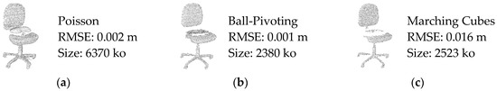
Figure 16. 3D modelling by triangulation. (a) Poisson reconstruction [115]; (b) Ball-pivoting approach [116]; (c) Marching-Cubes approach [117].

As for ${\mathcal{M}}_{3DM}$, our 3D data mining approach provides interesting results concerning the SIM dataset, but the extension to the real-world case presents many challenges. Primarily, the fact that the model does not exist in the database makes it necessary to search for a close candidate and to accommodate intra-${\mathcal{E}}_i$ variability. Secondly, the heterogeneity in shapes and forms within the database presents some cases that our algorithm cannot handle, typically when two shapes have a ${\mathcal{M}}_{L0}$ match, the distinction can provide a False Positive. The mining results, while assessing the fit’s precision, are illustrated in Figure 17.

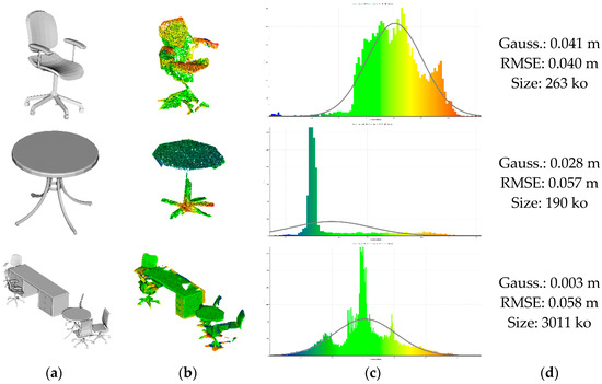
Figure 17. 3D modelling accuracy of the hybrid model. (a) constitutes the results of the 3D modelling through database mining; (b) presents the color-coded deviations to the corresponding model in (a), and studied by repartition in (c); gaussian, deviation and size are presented in (d).

We notice that using the different LoDs for the models within the shape matching approach makes it possible to extract candidates whose function best fits the indoor scenario. However, the obtained deviations to the S3-DIS point cloud range between 4 and 6 cm, which can limit the scenarios of use. Yet, it is important to note that those numbers are heavily influenced by the very high noise of the S3-DIS dataset, as well as the large occluded areas. Indeed, one advantage of this 3D mining mechanism is that it provides exhaustive representations from existing models, benefiting asset-management applications. Finally, the proposed methodology makes it possible to reconstruct a global 3D model (Figure 1C, Section 3.4), as analyzed and illustrated in Figure 18.

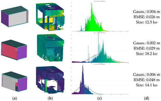
Figure 18. 3D area-decomposed global model of S3-DIS in $({\mathcal{M}}_{L0},{\mathcal{M}}_{L1})$. (a) constitutes the results of the 3D reconstruction modelling; (b) presents the color-coded deviations to (a): (c) represent the deviation analysis; (d) regroups main indicators.

We notice that RMSE deviations for $({\mathcal{M}}_{L0},{\mathcal{M}}_{L1})$ range from 2 cm to 5 cm, which correlates with the scanning method accuracy. On top, the modelling approach which leverages primitives produces an “as-built” reconstruction and therefore does not model small deviations relative to the global assemblage. If we look closely at the reconstruction of a hybrid $({\mathcal{M}}_{L1},{\mathcal{M}}_{3DM})$ global model, as illustrated in Figure 19, we first notice a very good trade-off between precision reconstruction and size, which is given by its hybrid nature. Moreover, we obtain a coherent watertight CSG assembly usable for simulations, as well as 3D printing. On top, the different relations between components allow a selectivity for this printing task.

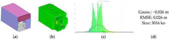
Figure 19. 3D modelling accuracy over the hybrid model. (a) constitutes the results of the 3D modelling through database mining; (b) presents the color-coded deviations to the corresponding model (a) and studied by repartition in (c), and the main indicators are presented in (d).

If we compare this to the existing Poisson’s modelling approach (Figure 20), we see that the reconstruction’s achieved precisions are often better. Moreover, the size on disk is much larger for the Poisson’s reconstruction. An interesting approach would be to combine a triangulation mechanism such as Poisson to account for small deviations which would extend to “as is” scenarios vs. “as-built”.

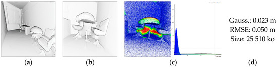
Figure 20. Poisson reconstruction of the S3-DIS dataset. (a) Global view; (b) High sensitivity to noise and occlusion; (c) Poisson’s deviation analysis; (d) main indicators.

By looking at (b) from Figure 20, we also note the high sensitivity to noise and occlusion in the analyzed dataset. This is particularly striking for the S3-DIS dataset and strengthen the robustness of our approach to these common artifacts (Figure 21).

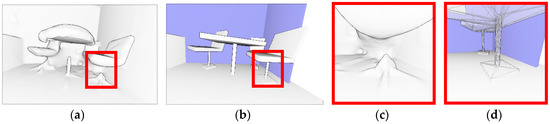
Figure 21. Noise and occlusion sensitivity. (a,c) shows a Poisson’s reconstruction; (b,d) shows the $({\mathcal{M}}_{L0},{\mathcal{M}}_{L2})$ reconstruction.

In the next sub-section, we will investigate the performance and implementation aspects of our approach.

4.3. Computation Time

We made a prototype implementation of the algorithms described in this paper in different programming languages. All the developments regarding the ACO were made in Java. The different application layers were built on top of RDF and ARQ API of Jena Apache (Java). Jena is an OWL-centric framework that is particularly well suited for our ontology, more so than OWLAPI, which is RDF-centric. The software Protégé was used as an interface to construct the ACO ontology. The part-segmentation, multi-LoD modelling and database matching were implemented in python using a minimal number of libraries: numpy (for numeric calculations), scikitLearn (for least squares, PCA analysis and signal analysis), matplotlib (for visualization), laspy (for point cloud loading), networkx (for graph and connectivity inference), psycopg2 (for a link to the SPC in-base data, stored in PostgreSQL) and rdfLib (for a connection to RDF triplestore). Visualization and rendering were conducted using Three.js or CCLib. All the experiments were conducted on a computer with an Intel Core i7 at 3.30 GHz and 32 GB of RAM. The exchange of information was made through a language processing module which can link SQL statements to JSON, RDF and OWL data, and be manually extended for natural language processing.

The running times (Figure 22) for the examples presented in this paper, as well as some additional experimental datasets, range from some seconds for the simpler shapes to several minutes for the more complex shapes. On average, the approach takes 85 s for the SIM dataset, 32 s for the DAT dataset, and 16 s for the S3-DIS dataset. Only one thread was used for the computation. The total time depends essentially on the size of the point cloud, and therefore the voxelization level retained. We note that there are some threshold and parameters that were determined empirically from our observation, and often their definition has an impact on the runtime. Relatively, the ontology information extraction and inference is quick, followed by the calculation and features in the point cloud (for part-segmentation). The voxelization is the part that consumes the most memory, but this can be further optimized by parallelizing its calculation. The structure is already ready for parallel processing. The data mining step can take up to 30 s for looking up 900 models in the off file format and provide the ranking as well as the necessary transformation parameters. Such a search can also be optimized if the models have previously been indexed. The CSG integration is quite fast, and is usually done in under 5 s. The full workflow from SPC data extraction to multi-LoD modelling and shape matching takes around 5 min for a full scene. The IFC file creation is made based on attributes in the JSON file format using the FreeCAD python wrapper.

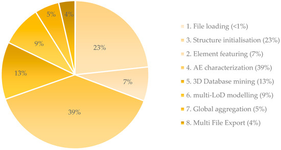
Figure 22. Relative time processing regarding the main elements of the 3D modelling engine.

4.4. Limitations

In an attempt to provide a clear list of research directions, we identified ten main points that could be further investigated:

• In our approach, we consider planar shapes only or manufactured shapes. It would be interesting to extend the method to more complex parametric representations as reviewed in Section 2.1.
• We consider the initial segmentation perfect. While the proposed algorithms are robust to false positives on planar shapes, handling failure cases that can arise when detecting furniture elements would make it possible to extend the depth of the framework.
• In our comparison and results analysis, we noticed deviations with elements which present a non-planar morphology. Adding a layer of shape deformation processing to best fit shapes is an opening to provide a compact hybrid model.
• The ACO was defined using expert knowledge, shape grammars and standards in use in Europe, and thus presents limitations linked to knowledge standardization. Extending the “standards” and features through machine learning could help to better generalize.
• Our voxel-based clustering approach is dependent on the underlying point data and density, and therefore it can have a high memory footprint, and thus, time execution. We are investigating the parallelization of computation to alleviate the processing and extend it to multi-LoD octree-based analysis.
• The binning and model fitting steps (Section 3) depend on the initial axis orientation’s determination. Extending its sturdiness to highly noisy and non-uniform point sampling would extend the flexibility of the workflow.
• The considerations in this paper and tests were conducted in indoor built environments only. Research to extend it to other scenes and outdoor scenarios is compelling.
• Non-standard shapes are difficult to describe through a knowledge-based approach. This limitation comes from the nature of ontologies to be integrated in standardization and interoperability workflows. One solution would be to compute robust features through a learning network on the existing set of 3D shapes.
• In our experiments, we mainly considered gravity-based scenes with an initial constraint regarding the object orientation. A global registration method would give additional flexibility about the prerequisites for the input dataset.
• We used the ACO for guiding the modelling process only. Due to its conception, it could be used as an ontology of classification to classify a point cloud in elements described within the OWL.

5. Perspectives

Admittedly, the present work merely takes one step forward in solving the general problem of 3D point cloud modelling. It raises several research directions described in Section 4.4, which arise from several identified limitations. It is important to note that our approach is based on a contextual analysis of our environment, looking at how elements interact with each other. As such, extending the methodology needs a generalization effort with regard to knowledge processing. Indeed, as it is based on an ACO knowledge representation of a specific application, the establishment of the ontology as it stands can in turn limit the interoperability with other domains. However, the approach shows how the context and all its implications regarding object relationships can be used for efficiently modelling point clouds. Going into detail, the initial characterization of input shapes needs to be sufficiently meaningful, especially the part-segmentation for AE. Furthermore, stitching parts together as models, especially for man-made shapes, is quite a difficult problem. It often requires the resolution of topological inconsistencies between parts, and the global problem is still an active research area. Our current solution to part assemblage is undeniably simplistic; thus, tackling the general problem presents interesting directions for future research. We are seeing a rapid accumulation of 3D models, yet most of these are not semantically described, and solely represent geometric shapes. We believe that the analogy to a set of shapes as presented in Section 3.4 is a great way to achieve shape retrieval and semantic completion. It can also be used for producing new variations of existing objects, as observed by Xu et al. [96]. As shown in this paper, context-based categorization can be an effective means to this end. Also, the Description Logic’s (DL) complexity of the ACO ontology is SHOIQ(D), a naming convention in Description Logic describing the complexity of reasoning in a knowledge base (Each character in the naming convention means that a logic constructor is used). OWL2 and its defined relations are the highest level of definition currently defined by OGC specifications. Therefore, in terms of calculation complexity, the proposed ontology features high-level semantic definition, which necessitates a heavy calculation process. To reduce this complexity, functional (F), inverse (I), reflexive and disjoint (R) relations will be rethought as much as possible in future work. It is worth mentioning that, while we use the KR for guiding the modelling engine in this work, it can also be used as a classification ontology. Pellet [118] or HermiT [119] reasoners are required because of their support of OWL2 and SWRL built-in functions.

Our part-based segmentation mechanism cannot efficiently handle non-standardized conception, which presents problems with regard to precise identification. On top, complex configurations such as folding chairs are currently not processed by our modelling engine. This could be solved by extending our ACO or through 3D database mining (if models exist in database). Our 3D shape matching procedure is also very interesting for two reasons. Firstly, by using topology, feature similarity and contextual information, we can recognize similar shapes within a given space, which provides a new way of modelling incomplete scenes or conducting variability analysis. Secondly, by looking up a 3D database, we can in turn extract the attached semantics to the fitted candidates and enrich the semantics of the 3D models as well as the underlying point cloud. Finally, it can be used as a means not only to reconstruct and model an object as a B-Rep or primitive-based representation, but to create an open link on the database model and its affiliate information. Indeed, this makes it possible to extract the added information (dimensions, price, availability, etc.) that a hosting database stores for asset management. This provides a great opening to interconnected networks of information that transit and avoid unnecessary multi-existence.

The scalability to bigger building complexes was proven using the real-world datasets; however, as indicated, the efficiency could be improved by using a better implementation. We focused on a geometry from terrestrial sensors with varying quality, but we intentionally left out color and texture due to their high variability in representativity. However, it could be useful in future considerations in order to better describe shapes, or as a means to extract better feature discrimination. Finally, in our approach, we tried to keep in mind the final use of the extracted 3D models, similarly to [47]. Whether the goal is the production of indoor CAD models for visualization, more schematic representations that may be suitable for navigation or BIM applications, or simply for scene understanding and object localization, in all these scenarios, the representation of the final objects differs, but the workflow of our modelling engine is particularly well adapted to generating several shape representations coupled with object relationships.

To our eyes, one of the most important perspectives concerns the interoperability of the approach within the SPC Infrastructure, acting as a module. Indeed, both are concerned with domain generalization, and the ability to extend workflows to all possible applications. Shape representation at different granularities is a step toward such a flexible use of semantically rich point cloud data. The 3D representation variability given by our multi-LoD approach provides high flexibility when we look at attaching geometries to a subset of points (specifically class instances). This in turn provides queries and filtering capabilities which offer better insight for a new range of scenarios. It also shows how the SPC Infrastructure can be used to provide deliverables for applications such as BIM modelling, virtual inventories or 3D mapping.

6. Conclusions

We presented an automatic method for the global 3D reconstruction of indoor models from segmented point cloud data. Our part-to-whole approach extracts multiple 3D shape representations of the underlying point cloud elements composing the scene before aggregating them with semantics. This provides a full workflow from pre-processing to 3D modelling, integrated in a knowledge-based point cloud infrastructure. This makes it possible to leverage domain knowledge through a constructed applicative context ontology for a tailored object characterization at different conceptual considerations. Comprising a 3D modelling step including shape fitting from ModelNet10 for furniture, our approach acts as an expert system which outputs different obj files as well as a semantic tree. The framework contributes an IFC-inspired as-built reconstruction of the global scene usable by reasoners for automatic decision-making.

References

- Gordon, S.J.; Lichti, D.D.; Stewart, M.P.; Franke, J. Modelling point clouds for precise structural deformation measurement. Int. Arch. Photogramm. Remote Sens. 2004, 35, B5. [Google Scholar]
- Bosche, F.; Haas, C.T.; Akinci, B. Automated Recognition of 3D CAD Objects in Site Laser Scans for Project 3D Status Visualization and Performance Control. J. Comput. Civ. Eng. 2009, 23, 311–318. [Google Scholar] [CrossRef]
- Bueno, M.; Bosché, F.; González-Jorge, H.; Martínez-Sánchez, J.; Arias, P. 4-Plane congruent sets for automatic registration of as-is 3D point clouds with 3D BIM models. Autom. Constr. 2018, 89, 120–134. [Google Scholar] [CrossRef]
- Labsch, M.; Kr, K.; Grash, F.; Kohl, S. Content Creation for a 3D Game with Maya and Unity 3D. In Proceedings of the 15th Central European Seminar on Computer Graphics, Viničn, Slovakia, 2–4 May 2011. [Google Scholar]
- Braun, E. System and Method for Cross-Platform and Cross-Game Virtual Asset Creation and Management. U.S. Patent 13/430,518, 27 September 2012. [Google Scholar]
- Dietenbeck, T.; Torkhani, F.; Othmani, A.; Attene, M.; Favreau, J.-M.M. Multi-layer ontologies for integrated 3D shape segmentation and annotation. In Studies in Computational Intelligence; Springer: Cham, Switzerland, 2017; Volume 665, pp. 181–206. [Google Scholar]
- Cao, Y.; Lu, F. Three-Dimensional Modeling for Buildings Evacuation Management. Bachelor’s Thesis, University of Gävle, Gävle, Sweden, 2012. [Google Scholar]
- Hinks, T.; Laefer, D.F.; Carr, H. Viability Considerations for the Application of Aerial LiDAR for Infrastructure Documentation and Monitoring. In Proceedings of the Transportation Research Board 87th Annual Meeting, Washington, DC, USA, 13–17 January 2008. [Google Scholar]
- Adjiski, V.; Mirakovski, D.; Despodov, Z.; Mijalkovski, S. Simulation and optimization of evacuation routes in case of fire in underground mines. J. Sustain. Min. 2015, 14, 133–143. [Google Scholar] [CrossRef]
- Lee, J.; Zlatanova, S. A 3D data model and topological analyses for emergency response in urban areas. In Geospatial Information Technology for Emergency Response; CRC Press: Boca Raton, FL, USA, 2008; pp. 143–167. [Google Scholar]
- Pu, S.; Zlatanova, S. Evacuation route calculation of inner buildings. In Geo-Information for Disaster Management; Springer: Berlin/Heidelberg, Germany, 2005; pp. 1143–1161. ISBN 3540249885. [Google Scholar]
- Daniel, S.; Harrap, R.; Power, M. Getting Into Position: Serious Gaming in Geomatics. In World Conference on E-Learning in Corporate, Government, Healthcare, and Higher Education; Association for the Advancement of Computing in Education: Waynesville, NC, USA, 2009; Volume 2009, pp. 213–219. [Google Scholar]
- Conconi, A.; Ganchev, T.; Kocsis, O.; Papadopoulos, G.; Fernández-Aranda, F.; Jiménez-Murcia, S. PlayMancer: A serious gaming 3D environment. In Proceedings of the IEEE 4th International Conference on Automated Solutions for Cross Media Content and Multi-Channel Distribution, Axmedis 2008, Florence, Italy, 17–19 November 2008; pp. 111–117. [Google Scholar]
- Escarieu, F.; Pousset, Y.; Aveneau, L.; Vauzelle, R. Outdoor and indoor channel characterization by a 3D simulation software. In Proceedings of the 12th IEEE International Symposium on Personal, Indoor and Mobile Radio Communications, PIMRC 2001 (Cat. No. 01TH8598), San Diego, CA, USA, 3 October–30 September 2001; Volume 1, pp. 105–111. [Google Scholar] [CrossRef]
- Cichon, D.J.; Zwick, T.; Lahteenmaki, J. Ray optical indoor modeling in multi-floored buildings: Simulations and measurements. In Proceedings of the IEEE Antennas and Propagation Society International Symposium (AP-S. Digest), Newport Beach, CA, USA, 18–23 June 1995; Volume 1, pp. 522–525. [Google Scholar]
- Korkalainen, M.; Sallinen, M.; Kärkkäinen, N.; Tukeva, P. Survey of wireless sensor networks simulation tools for demanding applications. In Proceedings of the IEEE 5th International Conference on Networking and Services, ICNS 2009, Valencia, Spain, 20–25 April 2009; pp. 102–106. [Google Scholar]
- Lauer, A.; Bahr, A.; Wolff, I. FDTD simulations of indoor propagation. In Proceedings of the IEEE Vehicular Technology Conference (VTC), Stockholm, Sweden, 8–10 June 1994; pp. 883–886. [Google Scholar]
- Kolbe, T.H.; Gröger, G.; Plümer, L. CityGML: Interoperable access to 3D city models. In Geo-Information for Disaster Management; Springer: Berlin/Heidelberg, Germany, 2005; pp. 883–899. ISBN 3540249885. [Google Scholar]
- Xiao, J.; Furukawa, Y. Reconstructing the World’s Museums. Int. J. Comput. Vis. 2014, 110, 243–258. [Google Scholar] [CrossRef]
- Zhou, C.; Liu, X.; Xue, F.; Bo, H.; Li, K. Research on static service BOM transformation for complex products. Adv. Eng. Inform. 2018, 36, 146–162. [Google Scholar] [CrossRef]
- Chen, C.; Zou, X.; Tian, M.; Li, J.; Wu, W.; Song, Y.; Dai, W.; Yang, B. Low cost multi-sensor robot laser scanning system and its accuracy investigations for indoor mapping application. ISPRS—Int. Arch. Photogramm. Remote Sens. Spat. Inf. Sci. 2017, 42, 83–85. [Google Scholar] [CrossRef]
- Liu, R.; Asari, V.K. 3D indoor scene reconstruction and change detection for robotic sensing and navigation. In Proceedings of SPIE—The International Society for Optical Engineering; Agaian, S.S., Jassim, S.A., Eds.; International Society for Optics and Photonics: Bellingham, WA, USA, 2017; Volume 10221, p. 102210D. [Google Scholar]
- Prieto, S.A.; Quintana, B.; Adán, A.; Vázquez, A.S. As-is building-structure reconstruction from a probabilistic next best scan approach. Robot. Auton. Syst. 2017, 94, 186–207. [Google Scholar] [CrossRef]
- Shen, S.; Michael, N.; Kumar, V. Autonomous Indoor 3D Exploration with a Micro-Aerial Vehicle. In Proceedings of the 2012 IEEE International Conference on Robotics and Automation, Saint Paul, MN, USA, 14–18 May 2012; pp. 1–7. [Google Scholar] [CrossRef]
- Zhu, Y.; Mottaghi, R.; Kolve, E.; Lim, J.J.; Gupta, A.; Fei-Fei, L.; Farhadi, A. Target-driven Visual Navigation in Indoor Scenes using Deep Reinforcement Learning. In Proceedings of the 2017 IEEE International Conference on Robotics and Automation (ICRA), Singapore, 29 May–3 June 2016; pp. 3357–3364. [Google Scholar] [CrossRef]
- Chow, J.C.K.; Peter, M.; Scaioni, M.; Al-durgham, M. Indoor Tracking, Mapping, and Navigation: Algorithms, Technologies, and Applications. J. Sens. 2018, 2018, 3–6. [Google Scholar] [CrossRef]
- Balado, J.; Díaz-Vilariño, L.; Arias, P.; Garrido, I. Point clouds to indoor/outdoor accessibility diagnosis. ISPRS Ann. Photogramm. Remote Sens. Spat. Inf. Sci. 2017, 4, 287–293. [Google Scholar] [CrossRef]
- Hayes-Roth, F.; Waterman Donald, A.; Lenat Douglas, B. Building Expert System; Addison-Wesley Longman Publishing Co., Inc.: Boston, MA, USA, 1983. [Google Scholar]
- Poux, F.; Billen, R. A Smart Point Cloud Infrastructure for intelligent environments. In International Society for Photogrammetry and Remote Sensing (ISPRS) Book Series; Lindenbergh, R., Belen, R., Eds.; CRC Press: Boca Raton, FL, USA, in press.
- Lehtola, V.; Kaartinen, H.; Nüchter, A.; Kaijaluoto, R.; Kukko, A.; Litkey, P.; Honkavaara, E.; Rosnell, T.; Vaaja, M.; Virtanen, J.-P.; et al. Comparison of the Selected State-Of-The-Art 3D Indoor Scanning and Point Cloud Generation Methods. Remote Sens. 2017, 9, 796. [Google Scholar] [CrossRef]
- Poux, F.; Neuville, R.; Hallot, P.; Billen, R. Model for reasoning from semantically rich point cloud data. ISPRS Ann. Photogramm. Remote Sens. Spat. Inf. Sci. 2017, 4, 107–115. [Google Scholar] [CrossRef]
- Poux, F.; Hallot, P.; Neuville, R.; Billen, R. Smart point cloud: Definition and remaining challenges. ISPRS Ann. Photogramm. Remote Sens. Spat. Inf. Sci. 2016, 4, 119–127. [Google Scholar] [CrossRef]
- Poux, F.; Neuville, R.; Van Wersch, L.; Nys, G.-A.; Billen, R.; Van Wersch, L.; Nys, G.-A.; Billen, R. 3D Point Clouds in Archaeology: Advances in Acquisition, Processing and Knowledge Integration Applied to Quasi-Planar Objects. Geosciences 2017, 7, 96. [Google Scholar] [CrossRef]
- van Oosterom, P.; Martinez-Rubi, O.; Ivanova, M.; Horhammer, M.; Geringer, D.; Ravada, S.; Tijssen, T.; Kodde, M.; Gonçalves, R. Massive point cloud data management: Design, implementation and execution of a point cloud benchmark. Comput. Graph. 2015, 49, 92–125. [Google Scholar] [CrossRef]
- Wu, Z.; Song, S.; Khosla, A.; Yu, F.; Zhang, L.; Tang, X.; Xiao, J. 3D ShapeNets: A deep representation for volumetric shapes. In Proceedings of the 2015 IEEE Conference on Computer Vision and Pattern Recognition (CVPR), Boston, MA, USA, 7–12 June 2015; pp. 1912–1920. [Google Scholar]
- Fathi, H.; Dai, F.; Lourakis, M. Automated as-built 3D reconstruction of civil infrastructure using computer vision: Achievements, opportunities, and challenges. Adv. Eng. Inform. 2015, 29, 149–161. [Google Scholar] [CrossRef]
- Zhang, D.; Lu, G. Review of shape representation and description techniques. Pattern Recognit. 2004, 37, 1–19. [Google Scholar] [CrossRef]
- Tang, P.; Huber, D.; Akinci, B.; Lipman, R.; Lytle, A. Automatic reconstruction of as-built building information models from laser-scanned point clouds: A review of related techniques. Autom. Constr. 2010, 19, 829–843. [Google Scholar] [CrossRef]
- Remondino, F. From point cloud to surface: The modeling and visualization problem. Int. Arch. Photogramm. Remote Sens. Spat. Inf. Sci. 2003, 34, 24–28. [Google Scholar]
- Cazals, F.; Giesen, J. Delaunay Triangulation Based Surface Reconstruction: Ideas and Algorithms. INRIA Rapp. Rech. 2004, 1, 1–45. [Google Scholar]
- Bommes, D.; Bruno, L.; Pietroni, N.; Levy, B.; Pietroni, N.; Puppo, E.; Silva, C.; Tarini, M.; Zorin, D. State of the Art in Quad Meshing. Eurogr. STARS 2012, 20, 1–24. [Google Scholar]
- Valero, E.; Adán, A.; Cerrada, C. Automatic Method for Building Indoor Boundary Models from Dense Point Clouds Collected by Laser Scanners. Sensors 2012, 12, 16099–16115. [Google Scholar] [CrossRef] [PubMed]
- Berger, M.; Tagliasacchi, A.; Seversky, L.; Alliez, P.; Levine, J.; Sharf, A.; Silva, C. State of the Art in Surface Reconstruction from Point Clouds. Eurogr. Star Rep. 2014, 1, 161–185. [Google Scholar]
- Berger, M.; Tagliasacchi, A.; Seversky, L.M.; Alliez, P.; Guennebaud, G.; Levine, J.A.; Sharf, A.; Silva, C.T. A Survey of Surface Reconstruction from Point Clouds. Comput. Graph. Forum 2017, 36, 301–329. [Google Scholar] [CrossRef]
- Canny, J. The Complexity of Robot Motion Planning; MIT Press: Cambridge, MA, USA, 1987; ISBN 9780262031363. [Google Scholar]
- Campbell, R.J.; Flynn, P.J. A survey of free-form object representation and recognition techniques. Comput. Vis. Image Understand. 2001, 81, 166–210. [Google Scholar] [CrossRef]
- Kim, Y.M.; Mitra, N.; Yang, D.-M.; Guibas, L. Acquiring 3D indoor environments with variability and repetition. ACM Trans. Graph. 2012, 31, 138. [Google Scholar] [CrossRef]
- Budroni, A.; Boehm, J. Toward automatic reconstruction of interiors from laser data. In Proceedings of the Virtual Reconstruction and Visualization of Complex Architectures (3D-ARCH), Trento, Italy, 25–28 February 2009. [Google Scholar]
- Pătrăucean, V.; Armeni, I.; Nahangi, M.; Yeung, J.; Haas, C. State of research in automatic as-built modelling. Adv. Eng. Inform. 2015, 29, 162–171. [Google Scholar] [CrossRef]
- Lee, J.; Son, H.; Kim, C.; Kim, C. Skeleton-based 3D reconstruction of as-built pipelines from laser-scan data. Autom. Constr. 2013, 35, 199–207. [Google Scholar] [CrossRef]
- Fayolle, P.A.; Pasko, A. An evolutionary approach to the extraction of object construction trees from 3D point clouds. Comput. Aided Des. 2016, 74, 1–17. [Google Scholar] [CrossRef]
- Adan, A.; Huber, D. 3D reconstruction of interior wall surfaces under occlusion and clutter. In Proceedings of the IEEE 2011 International Conference on 3D Imaging, Modeling, Processing, Visualization and Transmission, 3DIMPVT 2011, Hangzhou, China, 16–19 May 2011; pp. 275–281. [Google Scholar]
- Stamos, I.; Yu, G.; Wolberg, G.; Zokai, S. 3D modeling using planar segments and mesh elements. In Proceedings of the Third International Symposium on 3D Data Processing, Visualization, and Transmission, 3DPVT 2006, Chapel Hill, NC, USA, 14–16 June 2006; pp. 599–606. [Google Scholar]
- Lafarge, F.; Keriven, R.; Brédif, M. Insertion of 3-D-primitives in mesh-based representations: Towards compact models preserving the details. IEEE Trans. Image Process. 2010, 19, 1683–1694. [Google Scholar] [CrossRef] [PubMed]
- Lafarge, F.; Mallet, C. Creating large-scale city models from 3D-point clouds: A robust approach with hybrid representation. Int. J. Comput. Vis. 2012, 99, 69–85. [Google Scholar] [CrossRef]
- De Luca, L.; Veron, P.; Florenzano, M. Reverse engineering of architectural buildings based on a hybrid modeling approach. Comput. Graph. 2006, 30, 160–176. [Google Scholar] [CrossRef]
- Pu, S.; Vosselman, G. Knowledge based reconstruction of building models from terrestrial laser scanning data. ISPRS J. Photogramm. Remote Sens. 2009, 64, 575–584. [Google Scholar] [CrossRef]
- Schnabel, R.; Wahl, R.; Klein, R. Efficient RANSAC for Point Cloud Shape Detection. Comput. Graph. Forum 2007, 26, 214–226. [Google Scholar] [CrossRef]
- Schnabel, R.; Wessel, R.; Wahl, R.; Klein, R. Shape recognition in 3d point-clouds. In Proceedings of the 16th International Conference in Central Europe on Computer Graphics, Visualization and Computer Vision, Bory, Czech Republic, 4–7 February 2008; Volume 8. [Google Scholar]
- Poux, F.; Neuville, R.; Billen, R. Point cloud classification of tesserae from terrestrial laser data combined with dense image matching for archaeological information extraction. ISPRS Ann. Photogramm. Remote Sens. Spat. Inf. Sci. 2017, 4, 203–211. [Google Scholar] [CrossRef]
- Nurunnabi, A.; Belton, D.; West, G. Robust Segmentation in Laser Scanning 3D Point Cloud Data. In Proceedings of the IEEE 2012 International Conference on Digital Image Computing Techniques and Applications, Fremantle, Australia, 3–5 December 2012; pp. 1–8. [Google Scholar]
- Fischler, M.A.; Bolles, R.C. Random sample consensus: A paradigm for model fitting with applications to image analysis and automated cartography. Commun. ACM 1981, 24, 381–395. [Google Scholar] [CrossRef]
- Sanchez, V.; Zakhor, A. Planar 3D modeling of building interiors from point cloud data. In Proceedings of the IEEE International Conference on Image Processing, ICIP, Orlando, FL, USA, 30 September–3 October 2012; pp. 1777–1780. [Google Scholar]
- Nurunnabi, A.; Belton, D.; West, G. Robust segmentation for large volumes of laser scanning three-dimensional point cloud data. IEEE Trans. Geosci. Remote Sens. 2016, 54, 4790–4805. [Google Scholar] [CrossRef]
- Bosché, F. Plane-based registration of construction laser scans with 3D/4D building models. Adv. Eng. Inform. 2012, 26, 90–102. [Google Scholar] [CrossRef]
- Ni, H.; Lin, X.; Ning, X.; Zhang, J. Edge Detection and Feature Line Tracing in 3D-Point Clouds by Analyzing Geometric Properties of Neighborhoods. Remote Sens. 2016, 8, 710. [Google Scholar] [CrossRef]
- Budroni, A.; Boehm, J. Automated 3D Reconstruction of Interiors from Point Clouds. Int. J. Archit. Comput. 2010, 8, 55–74. [Google Scholar] [CrossRef]
- Macher, H.; Landes, T.; Grussenmeyer, P. From point clouds to building information models: 3D semi-automatic reconstruction of indoors of existing buildings. Appl. Sci. 2017, 7, 1030. [Google Scholar] [CrossRef]
- Ochmann, S.; Vock, R.; Wessel, R.; Klein, R. Automatic reconstruction of parametric building models from indoor point clouds. Comput. Graph. 2016, 54, 94–103. [Google Scholar] [CrossRef]
- Jung, J.; Hong, S.; Jeong, S.; Kim, S.; Cho, H.; Hong, S.; Heo, J. Productive modeling for development of as-built BIM of existing indoor structures. Autom. Constr. 2014, 42, 68–77. [Google Scholar] [CrossRef]
- Okorn, B.; Xiong, X.; Akinci, B.; Huber, D. Toward automated modeling of floor plans. In Proceedings of the Symposium on 3D Data Processing, Visualization and Transmission (3DPVT 10), Paris, France, 17–20 May 2010; Volume 2. [Google Scholar]
- Brédif, M.; Vallet, B.; Ferrand, B. Distributed Dimensonality-Based Rendering of LIDAR Point Clouds. In The International Archives of Photogrammetry, Remote Sensing and Spatial Information Sciences; Copernicus GmbH: La Grande Motte, France, 2015; Volume 40, p. 559. [Google Scholar]
- Nurunnabi, A.; Sadahiro, Y.; Lindenbergh, R. Robust cylinder fitting in three-dimensional point cloud data. Sciences 2017, 42, 63–70. [Google Scholar] [CrossRef]
- Kim, C.; Son, H.; Kim, C. Fully automated registration of 3D data to a 3D CAD model for project progress monitoring. Autom. Constr. 2013, 35, 587–594. [Google Scholar] [CrossRef]
- Wang, J.; Lindenbergh, R.; Menenti, M. SigVox—A 3D feature matching algorithm for automatic street object recognition in mobile laser scanning point clouds. ISPRS J. Photogramm. Remote Sens. 2017, 128, 111–129. [Google Scholar] [CrossRef]
- Liu, Y.-S.; Ramani, K. Robust principal axes determination for point-based shapes using least median of squares. Comput. Aided Des. 2009, 41, 293–305. [Google Scholar] [CrossRef] [PubMed]
- Ortiz, P.; Sánchez, H.; Pires, H.; Pérez, J.A. Experiences about fusioning 3D digitalization techniques for cultural heritage documentation. In Proceedings of the ISPRS Commision V Symposium, Image Engineering and Vision Metrology, Dresden, Germany, 25–27 September 2006. [Google Scholar]
- Nurunnabi, A.; Belton, D.; West, G. Diagnostic-robust statistical analysis for local surface fitting in 3D point cloud data. ISPRS Ann. Photogramm. Remote Sens. Spat. Inf. Sci. 2012, I-3, 269–274. [Google Scholar] [CrossRef]
- Mura, C.; Mattausch, O.; Jaspe Villanueva, A.; Gobbetti, E.; Pajarola, R. Automatic room detection and reconstruction in cluttered indoor environments with complex room layouts. Comput. Graph. 2014, 44, 20–32. [Google Scholar] [CrossRef]
- Arbeiter, G.; Fuchs, S.; Bormann, R.; Fischer, J.; Verl, A. Evaluation of 3D feature descriptors for classification of surface geometries in point clouds. In Proceedings of the IEEE International Conference on Intelligent Robots and Systems, Vilamoura, Portugal, 7–12 October 2012; pp. 1644–1650. [Google Scholar]
- Xu, Y.; Tuttas, S.; Hoegner, L.; Stilla, U. Reconstruction of scaffolds from a photogrammetric point cloud of construction sites using a novel 3D local feature descriptor. Autom. Constr. 2018, 85, 76–95. [Google Scholar] [CrossRef]
- Osada, R.; Funkhouser, T.; Chazelle, B.; Dobkin, D. Matching 3D models with shape distributions. In Proceedings of the SMI 2001 International Conference on Shape Modeling and Applications, Genova, Italy, 7–11 May 2001; IEEE Computer Society: Washington, DC, USA, 2001; pp. 154–166. [Google Scholar]
- Mitra, N.J.; Pauly, M.; Wand, M.; Ceylan, D. Symmetry in 3D geometry: Extraction and applications. In Computer Graphics Forum; Wiley/Blackwell: Hoboken, NJ, USA, 2013; Volume 32, pp. 1–23. [Google Scholar]
- Ikehata, S.; Yang, H.; Furukawa, Y.S. Structured indoor modeling supplementary material. In Proceedings of the 2015 IEEE International Conference on Computer Vision (ICCV), Santiago, Chile, 7–13 December 2015; pp. 1323–1331. [Google Scholar]
- Martinet, A.; Soler, C.; Holzschuch, N.; Sillion, F.X. Accurate detection of symmetries in 3D shapes. ACM Trans. Graph. 2006, 25, 439–464. [Google Scholar] [CrossRef]
- Kovács, I.; Várady, T.; Salvi, P. Applying geometric constraints for perfecting CAD models in reverse engineering. Graph. Models 2015, 82, 44–57. [Google Scholar] [CrossRef]
- Kazhdan, M.; Funkhouser, T.; Rusinkiewicz, S. Symmetry descriptors and 3D shape matching. In Proceedings of the 2004 Eurographics/ACM SIGGRAPH Symposium on Geometry Processing—SGP ’04, Nice, France, 8–10 July 2004; p. 115. [Google Scholar]
- Lafarge, F.; Descombes, X.; Zerubia, J.; Pierrot-Deseilligny, M. Structural approach for building reconstruction from a single DSM. IEEE Trans. Pattern Anal. Mach. Intell. 2010, 32, 135–147. [Google Scholar] [CrossRef] [PubMed]
- Nan, L.; Xie, K.; Sharf, A. A search-classify approach for cluttered indoor scene understanding. ACM Trans. Graph. 2012, 31, 137. [Google Scholar] [CrossRef]
- Bosché, F. Automated recognition of 3D CAD model objects in laser scans and calculation of as-built dimensions for dimensional compliance control in construction. Adv. Eng. Inform. 2010, 24, 107–118. [Google Scholar] [CrossRef]
- Besl, P.J.; McKay, N.D. A Method for Registration of 3-D Shapes. IEEE Trans. Pattern Anal. Mach. Intell. 1992, 14, 239–256. [Google Scholar] [CrossRef]
- Sharp, G.C.; Lee, S.W.; Wehe, D.K. ICP registration using invariant features. IEEE Trans. Pattern Anal. Mach. Intell. 2002, 24, 90–102. [Google Scholar] [CrossRef]
- Gruen, A.; Akca, D. Least squares 3D surface and curve matching. ISPRS J. Photogramm. Remote Sens. 2005, 59, 151–174. [Google Scholar] [CrossRef]
- Rabbani, T.; Dijkman, S.; van den Heuvel, F.; Vosselman, G. An integrated approach for modelling and global registration of point clouds. ISPRS J. Photogramm. Remote Sens. 2007, 61, 355–370. [Google Scholar] [CrossRef]
- Boykov, Y.; Kolmogorov, V. An experimental comparison of min-cut/max- flow algorithms for energy minimization in vision. IEEE Trans. Pattern Anal. Mach. Intell. 2004, 26, 1124–1137. [Google Scholar] [CrossRef] [PubMed]
- Xu, K.; Li, H.; Zhang, H.; Cohen-Or, D.; Xiong, Y.; Cheng, Z.-Q. Style-content separation by anisotropic part scales. ACM Trans. Graph. 2010, 29, 184. [Google Scholar] [CrossRef]
- Xu, K.; Zheng, H.; Zhang, H.; Cohen-Or, D.; Liu, L.; Xiong, Y. Photo-inspired model-driven 3D object modeling. In Proceedings of the ACM SIGGRAPH 2011 Papers (SIGGRAPH ’11), Vancouver, BC, Canada, 7–11 August 2011; p. 1. [Google Scholar]
- Zlatanova, S.; Van Oosterom, P.J.M.; Lee, J.; Li, K.-J.; Lemmen, C.H.J. LADM and INDOORGML for support of indoor space identification. ISPRS Ann. Photogramm. Remote Sens. Spat. Inf. Sci. 2016, 4, 257–263. [Google Scholar] [CrossRef]
- Lee, J.; Li, K.-J.; Zlatanova, S.; Kolbe, T.H.; Nagel, C.; Becker, T. OGC®indoorgml; Open Geospatial Consortium: Wayland, MA, USA, 2014. [Google Scholar]
- Vanlande, R.; Nicolle, C.; Cruz, C. IFC and building lifecycle management. Autom. Constr. 2008, 18, 70–78. [Google Scholar] [CrossRef]
- Bhojraj, S.; Lee, C.M.C.; Oler, D.K. What’s My Line? A Comparison of Industry Classification Schemes for Capital Market Research. J. Account. Res. 2003, 41, 745–774. [Google Scholar] [CrossRef]
- Quintana, B.; Prieto, S.A.; Adán, A.; Vázquez, A.S. Semantic scan planning for indoor structural elements of buildings. Adv. Eng. Inform. 2016, 30, 643–659. [Google Scholar] [CrossRef]
- Xiong, X.; Adan, A.; Akinci, B.; Huber, D. Automatic creation of semantically rich 3D building models from laser scanner data. Autom. Constr. 2013, 31, 325–337. [Google Scholar] [CrossRef]
- Xiong, X.; Huber, D. Using Context to Create Semantic 3D Models of Indoor Environments. In British Machine Vision Conference; BMVA Press: Durham, UK, 2010; pp. 1–11. [Google Scholar]
- Fisher, R.B. Applying knowledge to reverse engineering problems. Comput. Aided Des. 2004, 36, 501–510. [Google Scholar] [CrossRef]
- Son, H.; Kim, C. Semantic as-built 3D modeling of structural elements of buildings based on local concavity and convexity. Adv. Eng. Inform. 2017, 34, 114–124. [Google Scholar] [CrossRef]
- Xu, M.; Petrou, M. 3D Scene interpretation by combining probability theory and logic: The tower of knowledge. Comput. Vis. Image Understand. 2011, 115, 1581–1596. [Google Scholar] [CrossRef]
- Sainz, M.; Pajarola, R. Point-based rendering techniques. Comput. Graph. 2004, 28, 869–879. [Google Scholar] [CrossRef]
- Bui, G.; Le, T.; Morago, B.; Duan, Y. Point-based rendering enhancement via deep learning. Vis. Comput. 2018, 34, 829–841. [Google Scholar] [CrossRef]
- Kobbelt, L.; Botsch, M. A survey of point-based techniques in computer graphics. Comput. Graph. 2004, 28, 801–814. [Google Scholar] [CrossRef]
- Armeni, I.; Sener, O.; Zamir, A.R.; Jiang, H.; Brilakis, I.; Fischer, M.; Savarese, S. 3D Semantic Parsing of Large-Scale Indoor Spaces. In Proceedings of the IEEE International Conference on Computer Vision and Pattern Recognition, Las Vegas, NV, USA, 27–30 June 2016. [Google Scholar]
- Rusu, R.B.; Cousins, S. 3D is here: Point cloud library (PCL). In Proceedings of the 2011 IEEE International Conference on Robotic and Automation, Shanghai, China, 9–13 May 2011; pp. 1–4. [Google Scholar]
- Clementini, E.; Di Felice, P.; van Oosterom, P. A small set of formal topological relationships suitable for end-user interaction. In Advances in Spatial Databases; Abel, D., Chin Ooi, B., Eds.; Springer: Berlin/Heidelberg, Germany, 1993; pp. 277–295. ISBN 978-3-540-47765-5. [Google Scholar]
- Sutton, M.; Stark, L.; Bowyer, K. Function from visual analysis and physical interaction: A methodology for recognition of generic classes of objects. Image Vis. Comput. 1998, 16, 745–763. [Google Scholar] [CrossRef]
- Kazhdan, M.; Bolitho, M.; Hoppe, H. Poisson surface reconstruction. In Proceedings of the Eurographics Symposium on Geometry Processing, Sardinia, Italy, 26–28 June 2006; pp. 1–10. [Google Scholar]
- Bernardini, F.; Mittleman, J.; Rushmeier, H.; Silva, C.; Taubin, G. The ball-pivoting algorithm for surface reconstruction. Trans. Vis. Comput. Graph. 1999, 5, 349–359. [Google Scholar] [CrossRef]
- Lorensen, W.E.; Cline, H.E.; Lorensen, W.E.; Cline, H.E. Marching cubes: A high resolution 3D surface construction algorithm. In Proceedings of the 14th Annual Conference on Computer Graphics and Interactive Techniques (SIGGRAPH ’87), Anaheim, CA, USA, 27–31 July 1987; ACM Press: New York, NY, USA, 1987; Volume 21, pp. 163–169. [Google Scholar]
- Sirin, E.; Parsia, B.; Grau, B.C.; Kalyanpur, A.; Katz, Y. Pellet: A practical OWL-DL reasoner. Web Semant. Sci. Serv. Agents World Wide Web 2007, 5, 51–53. [Google Scholar] [CrossRef]
- Glimm, B.; Horrocks, I.; Motik, B.; Stoilos, G.; Wang, Z. HermiT: An OWL 2 Reasoner. J. Autom. Reason. 2014, 53, 245–269. [Google Scholar] [CrossRef]
© 2018 by the authors. Licensee MDPI, Basel, Switzerland. This article is an open access article distributed under the terms and conditions of the Creative Commons Attribution (CC BY) license (http://creativecommons.org/licenses/by/4.0/).