Article

Modeling the Distributions of Brightness Temperatures of a Cropland Study Area Using a Model that Combines Fast Radiosity and Energy Budget Methods

1
State Key Laboratory of Remote Sensing, Institute of Remote Sensing and Digital Earth, Chinese Academy of Sciences, Beijing 10010, China
2
College of Resources and the Environment, University of Chinese Academy of Sciences, Beijing 100049, China
3
Key Laboratory for Silviculture and Conservation of Ministry of Education, Beijing Forestry University, Beijing 100083, China
*
Authors to whom correspondence should be addressed.
Remote Sens. 2018, 10(5), 736; https://doi.org/10.3390/rs10050736
Submission received: 23 March 2018 / Revised: 29 April 2018 / Accepted: 4 May 2018 / Published: 10 May 2018

Abstract

:
Land surface temperatures (LSTs) obtained from remote sensing data are crucial in monitoring the conditions of crops and urban heat islands. However, since retrieved LSTs represent only the average temperature states of pixels, the distributions of temperatures within individual pixels remain unknown. Such data cannot satisfy the requirements of applications such as precision agriculture. Therefore, in this paper, we propose a model that combines a fast radiosity model, the Radiosity Applicable to Porous IndiviDual Objects (RAPID) model, and energy budget methods to dynamically simulate brightness temperatures (BTs) over complex surfaces. This model represents a model-based tool that can be used to estimate temperature distributions using fine-scale visible as well as near-infrared (VNIR) data and temporal variations in meteorological conditions. The proposed model is tested over a study area in an artificial oasis in Northwestern China. The simulated BTs agree well with those measured with the Advanced Spaceborne Thermal Emission and Reflection Radiometer (ASTER). The results reflect root mean squared errors (RMSEs) less than 1.6 °C and coefficients of determination (R2) greater than 0.7. In addition, compared to the leaf area index (LAI), this model displays high sensitivity to wind speed during validation. Although simplifications may be adopted for use in specific simulations, this proposed model can be used to support in situ measurements and to provide reference data over heterogeneous vegetation surfaces.

1. Introduction

Land surface temperature (LST) is always treated as a vital variable in the physical processes of surface-atmosphere interactions such as the energy budget and the hydrological cycle [1,2]. Currently, inversion with remote sensing data provides a vital means for obtaining global surface temperatures [3,4,5,6]. Many LST products have been evaluated and have been shown to have accuracies close to or less than 1.0 K [7,8,9,10,11]. However, because these retrieved LSTs usually correspond to a temperature state measured at specific spatial and temporal scales, how to fully use these retrieved results in applications such as evapotranspiration, climate change, and vegetation monitoring remains challenging [1].
For global-scale applications, the spatial resolution of thermal infrared (TIR) pixels collected by many geostationary or polar-orbit satellites is as coarse as 1.0 km or 5.0 km. In such cases, heterogeneous pixels are very common. Measurements of surface brightness temperatures (BTs) by the near-surface and airborne platforms display large differences in temperature among components while existing LST products represent only the average temperature states of satellite pixels [12]. Therefore, discrepancies between the temperatures of components and the results for individual pixels are inevitable. Kimes found that the deviation between nadir sensor BTs and vegetation BTs over a soybean canopy can reach up to 11 °C at midday [13]. Over mixed pixels that cover vegetation and urban areas, the temperature differences between components can reach up to 20 °C [14]. This level of discrepancy is not conducive to quantitative applications such as precision agriculture and sustainable urban design, which typically require finely resolved LSTs. In addition, the lack of a surface temperature distribution limits our understanding of the accuracy of coarse-scale LST products over heterogeneous surfaces due to scale problems.
In the visible and near-infrared (VNIR) domain, high-resolution images can be applied to obtain the distributions of reflectance within coarse-scale pixels [15,16]. This strategy is proposed mainly because the surface reflectance typically varies only slightly over short periods. However, LSTs display high sensitivity to the sun’s location and atmospheric instability. Therefore, the temporal variations in LSTs are more desirable than the LSTs at a specific temporal node when a satellite passes overhead [17,18]. Since the temperatures of surface components may respond differently to meteorological changes, surface heterogeneities increase the complexity of the transfers of radiation and energy within pixels. Currently, in situ experiments for the temporal and spatial variations in LSTs are limited.
Model-based approaches can help narrow the gap between the spatial-temporal variability of LSTs and practical applications. Three-dimensional (3-D) models seem suitable to explain the complex nature of satellite pixels, which may contain different types of landscapes [19,20,21]. Currently, many models have been proposed that aim to consider heterogeneous scenes and participate in the radiative transfer model intercomparison (RAMI) project [22]. For the temporal variability of LSTs, energy budget (EB) methods are typically incorporated [23,24,25,26]. This kind of model can be viewed as a tool that combines information on surface structure and diurnal changes in meteorological conditions. To study the temporal variability in the emissions from row-planted crops, Bian et al. proposed a quasi-3-D model that combines a 3-D radiosity model, a thermal radiosity-graphics combined model (TRGM), and EB methods. The combined model is named TRGM-EB) [27]. This model fully considers the effects of surface heterogeneities on radiative transfer. However, this combined model is not suitable for scenes on the scale of satellite pixels because it is slow to run and has high computer memory requirements. Addressing these shortcomings would enable the TRGM-EB model to be applied to study the distributions of surface temperatures within individual satellite pixels.
Huang et al. proposed a fast radiosity model known as the Radiosity Applicable to Porous IndiviDual Objects (RAPID) model in which the many facets that were previously used to represent small leaves are replaced with porous plant objects to improve the running speed of the model [28]. When large-scale scenes are considered, the RAPID model appears to be more suitable to be combined with EB methods than the TRGM. Therefore, we explore the application of a model (hereafter named RAPID-EB) that combines the RAPID model with EB methods to simulate surface BTs using both fine-scale VNIR data and in situ measured meteorological parameters. An artificial oasis in the middle reaches the Heihe River and is selected for investigation in a case study. In this study area, the spatial distribution of the BTs estimated using the RAPID-EB model and is evaluated using Advanced Spaceborne Thermal Emission and Reflection Radiometer (ASTER) TIR data. In Section 2, the new combined model is described. In Section 3, a practical procedure is applied to the study area and an evaluation is performed. In Section 4, validation problems and potential applications of this model are discussed. Section 5 provides a short summary of the paper as a whole.

2. The RAPID-EB Model

The strategy of combining a radiosity model includes TRGM or RAPID and EB methods, which are based on the Soil Canopy Observation, Photochemistry, and an Energy Fluxes (SCOPE) soil-vegetation-atmosphere-transfer (SVAT) model [25]. The radiative transfer process in SCOPE is based on the Scattering by Arbitrarily Inclined Leaves (SAIL) framework and assumes a homogeneous vegetation canopy. For a row-planted maize canopy, the 4SAIL radiative transfer treatment used in SCOPE is replaced by the 3-D radiosity model TRGM in Reference [27]. The use of this model enables the accurate estimation of the net radiation of each facet over both homogeneous and heterogeneous scenes. In this paper, the TRGM is replaced by the RAPID model. Consistent with TRGM-EB, the new combined model mainly consists of two modules including radiative transfer and EB. These modules correspond to two processes. Specifically, component temperatures are entered and the net radiation of each facet is then calculated according to the radiation interactions among facets while the calculated net radiation is then divided into the turbulent and soil surface heat fluxes and the component temperatures are optimized according to the energy balance equation. After several iterations between these two processes, the thermodynamic equilibrium state of a given scene is characterized.

2.1. Radiosity Model

In a radiosity model, each of the facets mentioned above represents a basic unit and these units comprise complex scenes. The initial step in a radiosity model is to calculate the radiosity of a facet, which is defined as the radiation flux density that leaves the facet. The radiation interactions among facets in a generated scene can be described by the radiosity equation shown below [21].
B i = E i + x i j F i , j B j , i , j = 1 , 2 , , 2 n p
E i = [ F s ( i ) + F d ( i ) ] ρ i + [ F s ( i + n p ) + F d ( i + n p ) ] τ i + F e ( i )
where B i represents the radiosity of the surface facet i . E i represents the emittance, which consists of direct solar light ( F s ), atmospheric diffuse light ( F d ), and a self-emission term ( F e ), which is shown in Equation (2). x i represents the reflectance or transmittance depending on the orientations of facets i and j relative to each other. n p represents the number of facets in a scene, i + n p represents the other side of facet i, F i , j represents the viewing factor between facets i and j , and it denotes their radiation interaction intensity, which depends on their area and orientation relative to each other. A detailed description of the procedure used in estimating E i is provided in Equation [21]. Based on the radiosity equations of all facets, the multiple scattering radiation ( x i j F i , j B j ) can be calculated using a Gauss-Seidel optimization method. The net radiation of one side of facet i can then be calculated using the equations below.
R n , s ( i ) = λ F s ( i , λ ) / a ( i , θ s ) + F d ( i , λ ) + j F i , j B j ( λ ) F e ( i , λ ) [ 1   ρ ( i , λ ) τ ( i , λ ) ]
R n , h ( i ) = λ F d ( i , λ ) + j F i , j B j ( λ ) F e ( i , λ ) [ 1   ρ ( i , λ ) τ ( i , λ ) ]
where R n ( i ) represents the net radiation of one side of facet i . The subscripts s and h represent the sunlit and shaded portions of a facet, respectively, a ( i , θ s ) represents the viewing fraction of facet i in the solar direction θ s , and λ represents the spectral wavelength. For leaf components, the total net radiation of facet i is R n ( i ) + R n ( i + n p ) . For soil or building components, the net radiation of facet i is R n ( i ) . In this model, the total net radiation is calculated by integrating from the visible domain (0.4 μ m ) to the infrared domain (50 μ m ). Since the viewing factors among the facets are independent of the wavelength and Sun location, their calculated values can be used for all spectral bands and temporal nodes. In this paper, the self-emission term ( F e ) in the infrared domain is calculated using the temperature ( T i ) and broadband emissivity ( ε i ) of each component, according to the Stefan-Boltzmann law.
F e ( i ) = ε i σ T i 4
where σ is the Stefan–Boltzmann constant, i.e., 5.6704 × 10 0 W m−2 K−4.

2.2. Energy Budget Methods

An EB module is incorporated to solve the difficulties that are encountered when obtaining surface component temperatures and simultaneously calculating surface heat fluxes. The core of the EB module is the energy balance equation, which is shown in the equations below.
R n = H λ Ε G
H = ρ a c ρ T s T a r a
λ Ε = γ q s ( T s ) q a r a + r s
T s ( t + t ) T s ( t ) = 2 ω Γ t G ( t ) - ω t [ T s ( t ) T s ¯ ]
where H and λ Ε represent the sensible and latent heat fluxes, respectively, which are estimated using Equation (6) and Equation (7) [2] and G represents the surface heat flux and its value for soil is estimated using a force-restore method, which was described by Equation (9) [25,29]. ρ a , c ρ ,   q a , and T a represent the density, heat capacity, humidity, and temperature of the air, respectively. r a and r s represent the aerodynamic resistance and surface (leaf stomatal) resistance, respectively. γ is the heat of evaporation of water, q s and T s are the surface humidity and temperature, respectively, t is the time interval, ω is the frequency of the diurnal cycle, Γ is the soil thermal inertia, and T s ¯ is the average annual temperature.
Over a mixed vegetation canopy, plants with different heights, leaf area index (LAI) values, and leaf angle distributions (LADs) may coexist. Therefore, we use a series of aerodynamic resistance values reported by Reference [30] for different leaf facets in this model. The storage of heat by leaves is not considered [31]. In general, the initial input of component temperatures does not satisfy the energy balance equation. The component temperatures are modified step by step, which is shown in the equations below.
T u p d a t e , i = T a + [ R n ( T i ) LE ( T i ) G ( T i ) ] r a ρ a c ρ
T i = T u p d a t e , i w + ( 1 w ) T i
where R n ( T i ) ,     L E ( T i ) ,     and   G ( T i ) represent the net radiation, latent heat flues, and soil surface heat fluxes of facet i when using the last temperature T i , respectively. T u p d a t e , i represents the temperature in H ( T i ) that satisfies the energy balance and T i represents the modified temperature. w represents the weight of T u p d a t e , i on T i . When the difference between R n ( T i ) and L E ( T i ) + G ( T i )   +   H ( T i ) is less than the required accuracy (1 W/m2) for all facets, the thermodynamic equilibrium state of the scene is assumed to have been achieved.

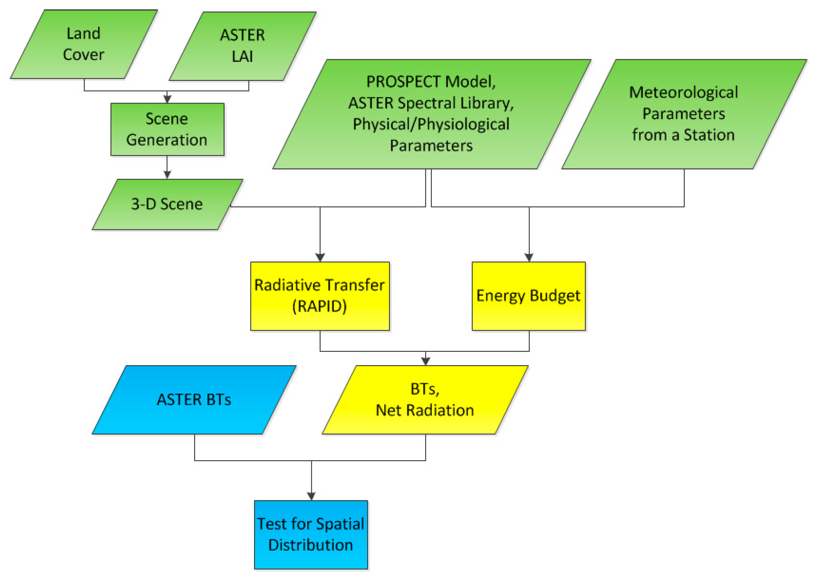
2.3. Combination of RAPID and Energy Budget Methods

In the TRGM, an exact 3-D vegetation canopy is typically used, which is composed of many trunks, branches, and small leaf facets. A modified extended L-system has been introduced for canopies of different vegetation types such as wheat and maize [21]. However, too many small leaf facets are necessary to produce a detailed forest canopy. Based on the descriptions provided above, the iteration of the radiative transfer and EB modules to achieve component temperatures satisfy the energy balance equation, which requires a considerable amount of computing time. Therefore, reducing the number of facets used can be a good means of improving computational efficiency and saving computer memory, which is the strategy used in RAPID [28].
Although the TRGM is replaced by the RAPID model, the RAPID-EB model inherits all of the processes included in TRGM-EB, i.e., Equations (1)–(8). The major improvement represented by the RAPID model uses plant objects to represent vegetation canopies [28]. Figure 1 shows an actual forest canopy and the illumination of plant objects. A plant object is composed of several horizontally arranged porous facets that represent a group of small leaf facets in each layer in a canopy. The gap frequency of a large porous facet is determined by the characteristics of leaves such as the LAI, the LAD, and the shapes of leaves. As a default approximation, the shape of a leaf is set to an equilateral triangle. Under this simplification, the heterogeneity of a scene is considered in terms of the spatial distribution and the shapes of plant objects, but the structure within a porous facet is considered to be homogeneous. When calculating transfers of radiation and energy, only these large porous facets are involved rather than the small leaf facets. This fact implies that a limited number of effective facets can be used to represent many actual facets inside a plant. Note that a 3-D scene that can be used in the TRGM can also be used in the RAPID model. For details on the RAPID model, refer to Reference [28].
In the TRGM-EB model, in order to consider large-scale scenes that contain different vegetation types, a simple discrete method is adopted to address horizontal heterogeneity. The use of this method causes discrepancies in simulations at the borders between types if the discretization is coarse. In the RAPID-EB model, all facets within a landscape are calculated using land cover information. Within a large-scale pixel, buildings may appear. In the radiative transfer process, only the outward sides of building facets can be viewed. These are similar to soil facets. The turbulent heat fluxes over urban areas have been analyzed by many authors [32,33,34,35]. In this paper, the heat fluxes from buildings are calculated based on Reference [32]. Over an urban area, the ratio between the roughness length for momentum and the building height is set to the default value of 1/10 and the ratio between the zero-plane displacement length and the building height set to the default value of 2/3. These two variables can also be calculated based on building geometry [36]. In addition, the latent heat fluxes from building facets are not considered.

2.4. Model Inputs and Outputs

Three types of inputs should be entered into the RAPID-EB model including 3-D scenes, component properties, and micrometeorological parameters. A graphical user interface (GUI) for generating complex 3-D scenes was previously developed by Huang et al [28,37]. This GUI includes predefined plant objects and other plant objects can be generated by using user-defined structural parameters. In this model, three main kinds of land cover are considered including areas of bare soil, vegetated areas, and built-up areas. The facet types within these land-cover types can be classified as soil, leaves, trunks, roofs, walls, and roads. When generating a scene, the initial step is to set the background area (soil) using many rectangular solid facets following the surface terrain. The plant objects mentioned above and a generated exact-structure crop canopy are then distributed over the vegetated area and the LAI, LAD, and leaf shape are defined for each porous facet. Within built-up areas, buildings are constructed by using solid facets. Each building is simplified as a cube in this paper. The component properties and meteorological parameters used in the RAPID-EB model are the same as those in the TRGM-EB model [27]. The component properties can be simply classified as optical and physical/physiological characteristics. During the radiative transfer process, the optical characteristics (reflectance and transmittance) of the components are essential inputs, according to Equation (1). The physiological properties of leaves are required for the transpiration process, which are related to leaf stomatal resistance [38,39]. The physical properties of soil and buildings are important factors when estimating the surface resistance [40]. The meteorological parameters that are required to drive the EB module can be obtained from a meteorological station.
Once the thermodynamic equilibrium of a scene is achieved, the temperatures and radiosity values of the sunlit and shaded areas of each facet can be obtained. Then the top-of-canopy (TOC) TIR radiance can be calculated as the average of the radiosity of all the facets within a field of view weighted by their visible fractions, which is shown below.
I ( v ) = i 2 n p B i π a r e a ( i ) · a ( i , θ v ) · | n i s v |   i 2 n p a r e a ( i ) · a ( i , θ v ) · | n i s v |
where a r e a ( i ) represents the area of facet i , a ( i , θ v ) represents the viewing fraction of facet i in the viewing direction θ v because facets may obscure each other and n i and s v represent the unit normal vector of facet i and the viewing direction, respectively. | n i s v | explains the projection of facet i relative to the viewing direction and a r e a ( i ) · a ( i , θ v ) · | n i s v | represents the weight of facet i for the TOC radiance. B i represents the efficient radiosity of facet i considering the sunlit fraction in the viewing direction and B i / π represents the radiance of facet i in the viewing direction because all the components are assumed to be Lambertian. In addition, the sensible and latent heat fluxes are calculated in the EB module, but they are not discussed in this paper.

3. Materials and Methods

A vital goal of this new combined model is to dynamically simulate the distributions of temperatures over complex surfaces. In this section, we assess the performance of the RAPID-EB model using TIR data obtained by the ASTER sensor. An artificial oasis in Northwestern China was selected as a study area. In addition, two days, which are 10 July 2012 and 2 August 2012, were selected for study. Both of these days fell within the summer vegetation growing season and were cloudless. In this evaluation, we did not use a cloud mask. An atmospheric correction of the observed TIR radiance values was performed by converting the top-of-atmosphere (TOA) values to the corresponding TOC values using the Moderate Resolution Atmospheric Transmission (MODTRAN) code [41,42]. The TOC TIR radiance values were then converted to BTs using the Planck function. The scheme that was used to test the combined model can be seen in Figure 2 and details are provided in the following subsections.

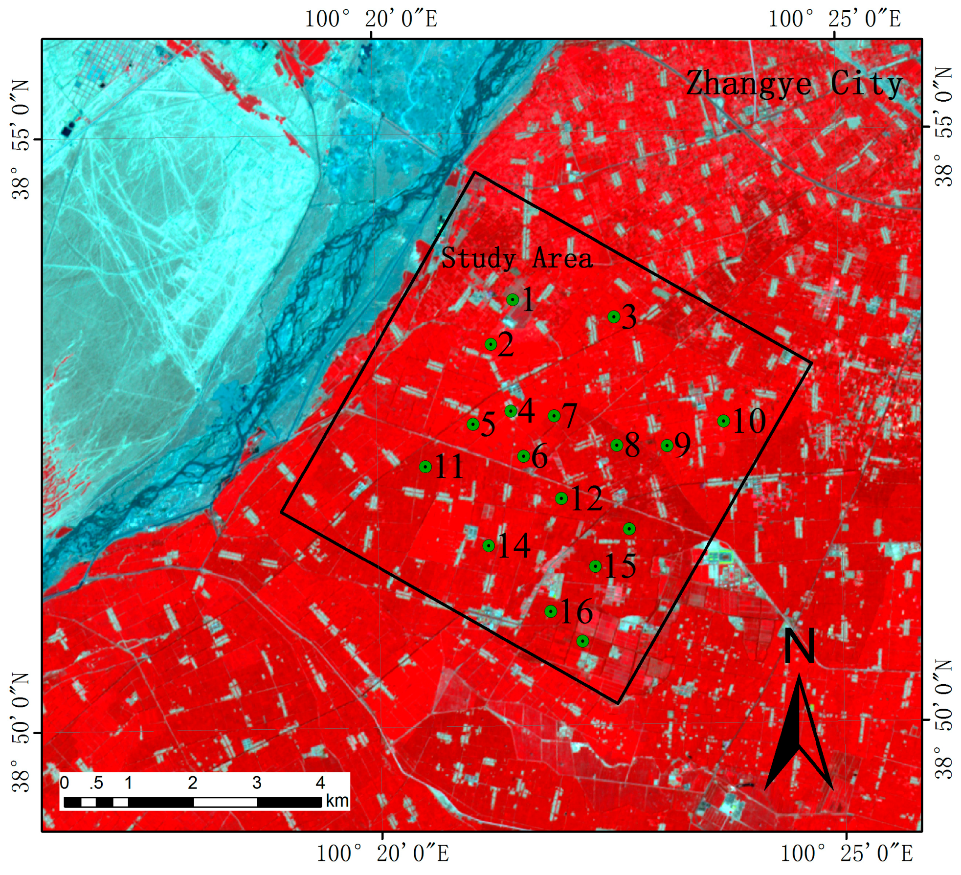
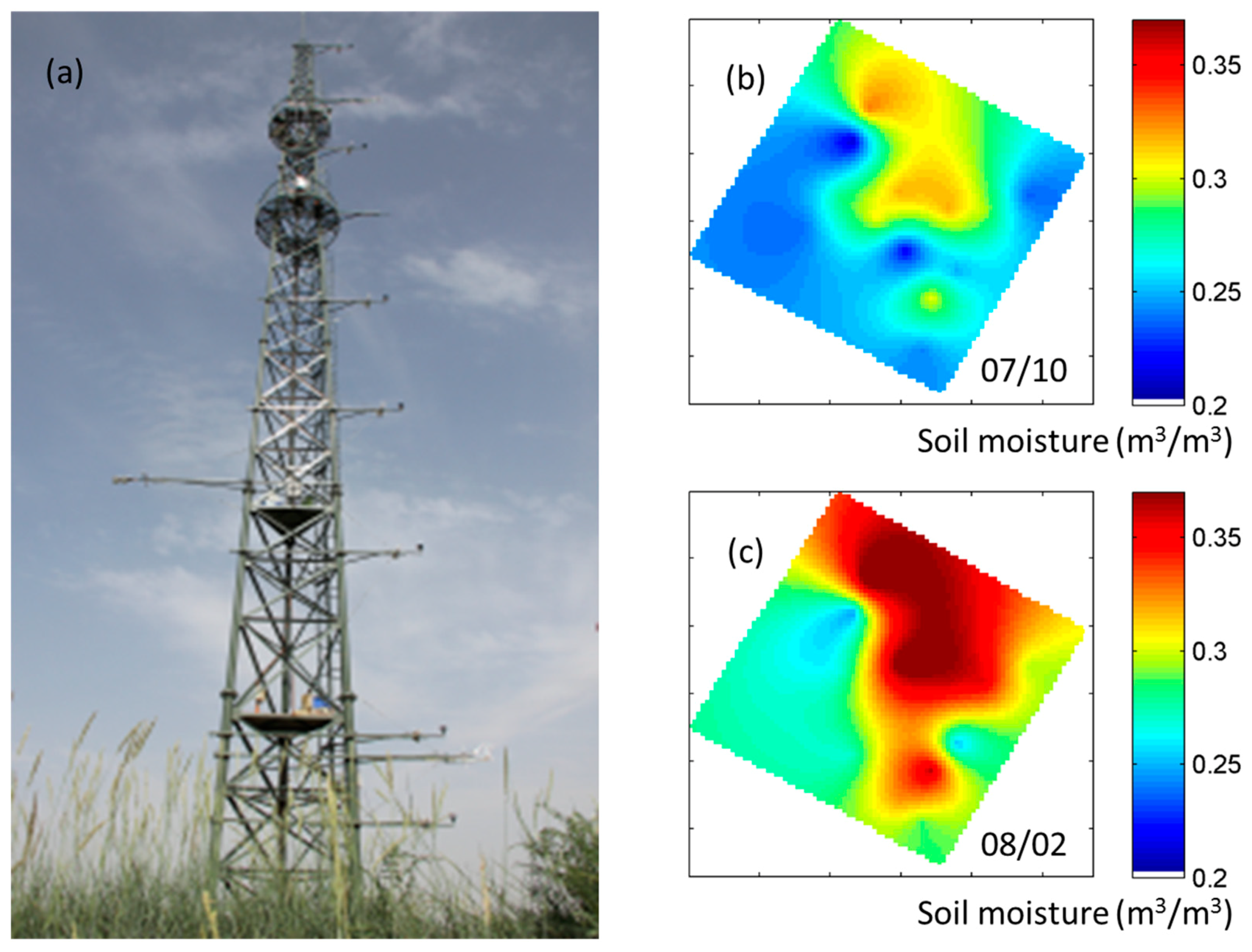
3.1. Experimental Site

In this paper, the area shown in Figure 3, which has a size of 6.25 km × 6.225 km, was selected for the evaluation exercise. This study area is located in an artificial oasis in the middle reaches of the Heihe River in the Gansu province of China. During the summer of 2012, this area was selected as a key experimental area where intensive and long-term observations were collected during the HiWATER (The Heihe Watershed Allied Telemetry Experimental Research) project [43]. During the summer, maize is the major agriculture crop and all of the vegetated area was assumed to be occupied by maize in the evaluation process. In addition, building and road pixels exist in this area. In this paper, the roads were represented as bare soil because most of these roads are paved with soil. The surface soil type is silty clay loam. The locations of seventeen automatic meteorological stations are shown in Figure 3 and these stations measured meteorological parameters during the HiWATER project [44]. This selected area is a typical irrigation district. The precipitation in this area is approximately 100–250 mm per year, but the potential evaporation is as high as 1200–1800 mm per year [43]. The annual average air temperature of this selected area is 280.45 K [45].

3.2. Data Sets

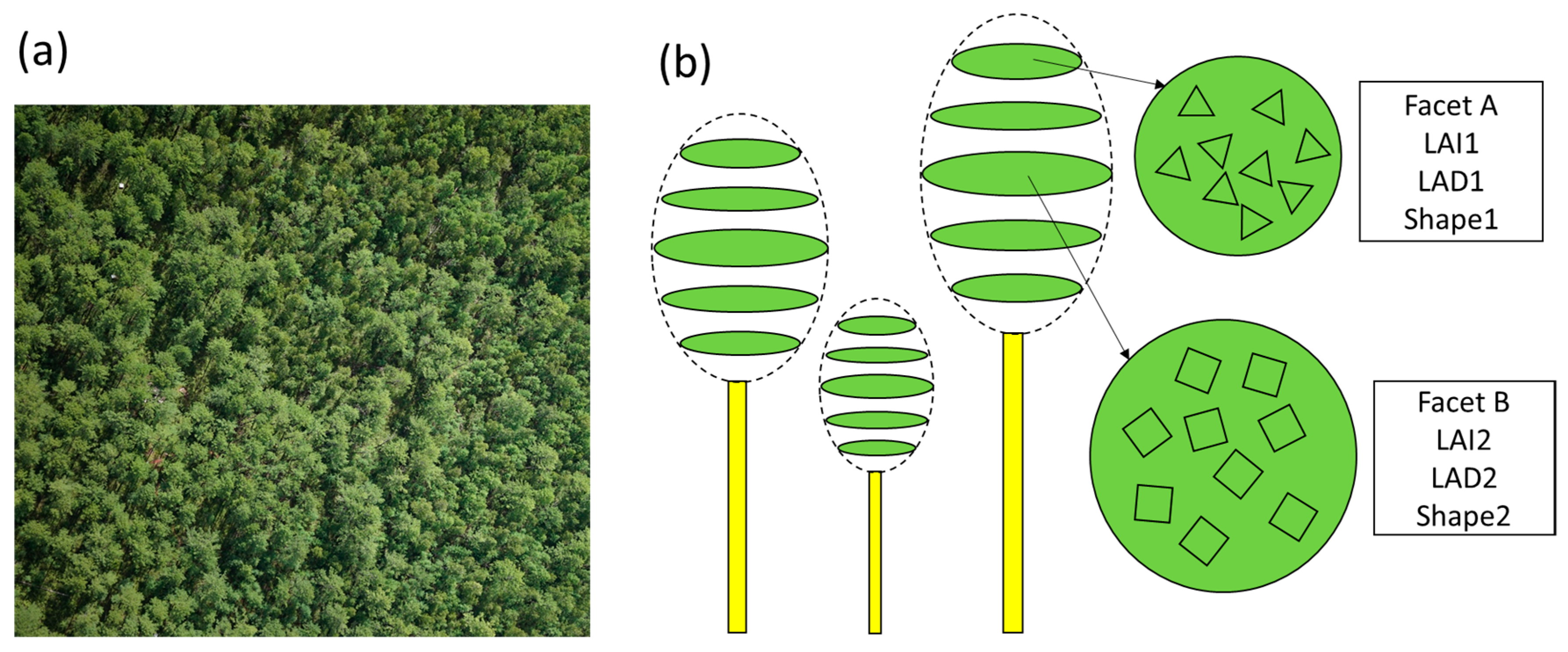
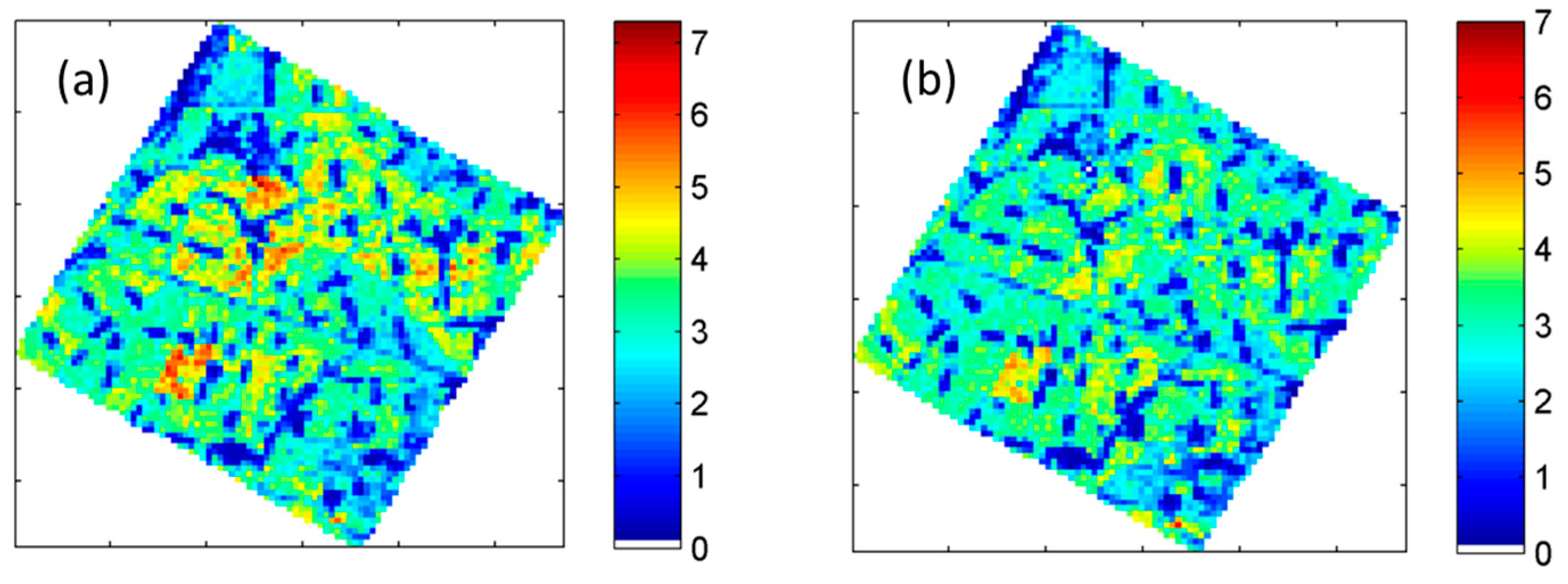
3.2.1. Scene Generation

This study area was treated as completely flat during the scene generation process. To save computer memory, the entire study area was divided into many sub-scenes with a size of 900 m × 900 m. To preserve the continuity between neighboring sub-scenes, the actual size of the sub-scenes was set to be slightly larger than 900 m × 900 m. The land cover information was obtained online at http://westdc.westgis.ac.cn [46,47]. The maize was planted in rows, but, during the period for which the evaluation was performed, the canopy was very dense. Therefore, this maize canopy was considered to be homogeneous. The LAI distribution within the study area was retrieved from ASTER VNIR images, which is shown in Figure 4 [48]. On 10 July 2012 and 2 August 2012, the average LAI values of the study area as a whole were 2.94 and 2.63, respectively. In addition, the corresponding average maize heights were 1.7 m and 2.0 m, respectively. These values were estimated by averaging measurements made near each automatic meteorological station. These average maize heights were used for all of the maize canopies in the generated scenes. In addition, the average height of 3.2 m was used for all of the buildings. Due to the limitations of the spatial resolution of LAI pixels, plant and building objects were set to a size of 30 m × 30 m. A spherical LAD was assumed for all of the plant objects.

3.2.2. Meteorological Data

The meteorological data were obtained from the automatic meteorological stations shown in Figure 3. Meteorological data were collected every 10 minutes and include the air temperature, air humidity, and air pressure at 5.0 m above the ground level. The wind speed and direction is 10.0 m above the ground level, the four-component radiation (downward/upward shortwave and longwave radiation) is 6.0 m above the ground level, and the soil moisture has depths of 2.0 cm and 4.0 cm. The Daman Super Station (i.e., station15) is a 40 m boundary-layer tower located at 100°22′ E, 38°51′ N. This station is surrounded by maize canopies, which is shown in Figure 5a and provides air temperatures and wind speeds at heights of 3.0 m, 20.0 m, 30.0 m, and 40.0 m. The air temperature, air humidity, air pressure, and wind speed values are considered to be the same over the study area as a whole and those obtained from the Daman Super Station were entered into the RAPID-EB model. The soil surface moisture was obtained by interpolating the measured values from the 17 automatic meteorological stations. Figure 5b,c show the spatial distribution of the soil surface (0 cm to 5 cm) moisture on the two selected days and this quantity was calculated by averaging the measured data at the 2.0-cm and 4.0-cm depths. The soil moisture mainly varied from 0.25 to 0.35 m3/m3, which represents well-irrigated conditions for agricultural crops.
In this paper, the BTs observed by the ASTER sensor were employed for evaluation and these values corresponded to approximately 12:15 Beijing time (12:13 and 12:19 Beijing time on 10 July and 2 August 2012, respectively). Therefore, the measured records that ranged from 12:10 to 12:20 Beijing time were used. The corresponding local time was approximately 10:35 and the two selected days were cloudless and feature air temperatures of 25.9 °C and 27.8 °C, respectively. The downward shortwave radiation values were as high as 925 W/m2 and 916 W/m2 with solar zenith angles of 21.5° and 25.6°, respectively. In addition, the corresponding wind speeds were 1.62 m/s and 0.90 m/s.

3.2.3. Component Properties

The optical properties of the components are important factors when estimating the net radiation of facets. The reflectance and transmittance of leaves in the VNIR domain were simulated by using the PROSPECT model with the input parameter values shown in Table 1 [49]. The VNIR properties of the other components were acquired from the ASTER spectral library [50]. The emissivity values of the components were retrieved using the Iterative Spectrally Smooth Temperature and Emissivity Separation (ISSTES) algorithm based on data measured using an ABB BOMEM MR304 Fourier transform infrared spectroradiometer [51]. In this paper, the five TIR bands of the ASTER sensor, i.e., 8.29 μm, 8.63 μm, 9.07 μm, 10.66 μm, and 11.32 μm, were all selected [52]. By resampling with spectral response functions, the channel emissivities of the components can be calculated, which is shown in Table 1.
The physical and physiological properties of components are mainly used to calculate the surface resistance and leaf stomatal conductivity. The leaf physiological properties were the same with the pre-defined empirical values of the SCOPE model [27,53]. In addition, the soil surface resistance was estimated using the surface moisture, which is shown in the equation below [40].
r s =   1.439 × 10 5 ( θ s a t θ 0 5 ) 3.14
where θ represents the soil water content. θ s a t and θ 0 5 represent the soil water content at saturation and the soil moisture of the top soil layer (0–5 cm), respectively. In our study area, θ s a t is set to 0.48 m3/m3. The soil surface moisture was also used to estimate the soil heat capacity ( ρ s c s ), which is shown in the equation below [54].
ρ s c s =   ρ d r y c d r y + ρ w c w θ 0 5
where ρ d r y c d r y and ρ w c w are the heat capacities of dry soil ( ~ ( 1 θ s a t ) × 2.1 × 10 6   J   kg 1   K 1 ) and water ( ~ 4.2 × 10 6   J   kg 1 K 1 ).

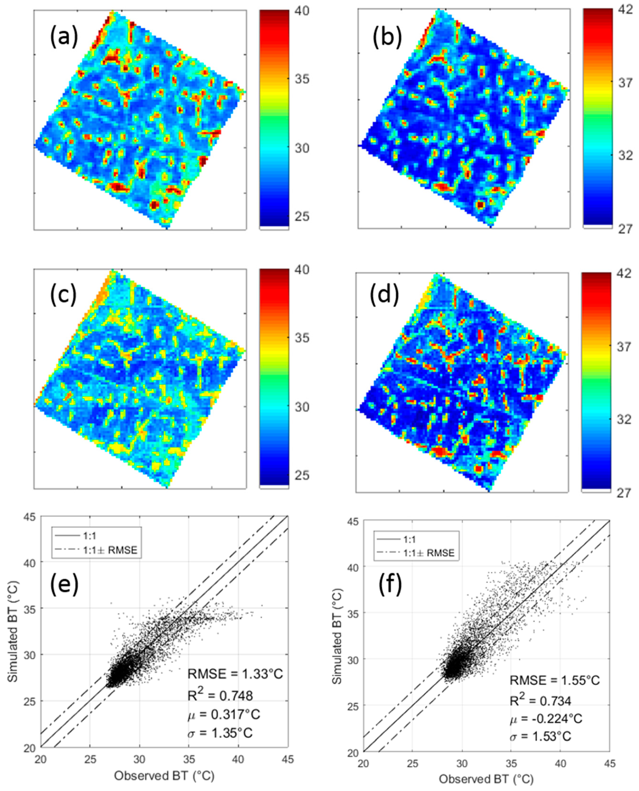
3.3. Evaluation for Temperature Distribution

The surface BTs were simulated with a spatial resolution of 90.0 m in order to match the ASTER pixels. In this paper, only pixels that were completely included within the study area were selected. Since the maximum viewing angle in an ASTER TIR image is only 8.55° [52], nadir observations were adopted for all of the simulated pixels.
Figure 6 shows the distributions of the observed and simulated BT values (11.32 μ m ) on the two selected days and their scatterplots. The corresponding statistics are shown in Table 2. The surface BTs on 10 July 2012 were slightly lower than those on 2 August 2012. Both the observed and simulated surface BTs displayed large ranges of values and the maximum BT difference was as large as 15 °C. Figure 6e,f shows scatterplots of the BTs between the observed and simulated pixels. The low RMSE values obtained for the two selected days (1.33 °C for 0710 and 1.55 °C for 0802) indicate that the RAPID-EB model displays acceptable performance when simulating surface BTs. In addition, the spatial distribution of the simulated BTs agreed well with those observed by the ASTER sensor. The corresponding coefficients of the determination (R2) value was greater than 0.73. In addition, similar evaluation results were obtained for the other ASTER bands where the RMSE values were less than 1.6 °C and the R2 values were greater than 0.70.
However, differences between the observed and simulated BTs also appeared. The building pixels with relatively large BTs displayed worse agreement than the vegetation pixels with relatively low BTs, which can be easily found in the scatterplots. The simulated BTs for the building pixels displayed similar values while their corresponding observed results substantially varied. Relative to 2 August 2012, this underestimate appeared for some of the simulated building pixels on 10 July 2012. In addition, the spatial distribution of the simulated vegetation BTs slightly differed from the observed BTs on 10 July 2012. Table 3 displays the evaluation results of the BTs (11.32 μ m ) for vegetation and building pixels. The RMSEs for buildings (2.11 °C and 1.73 °C) were larger than those for vegetation (1.14 °C and 1.20 °C). The RMSEs for bare soil were 2.66 °C and 1.96 °C on 10 July 2012 and 2 August 2012, respectively.

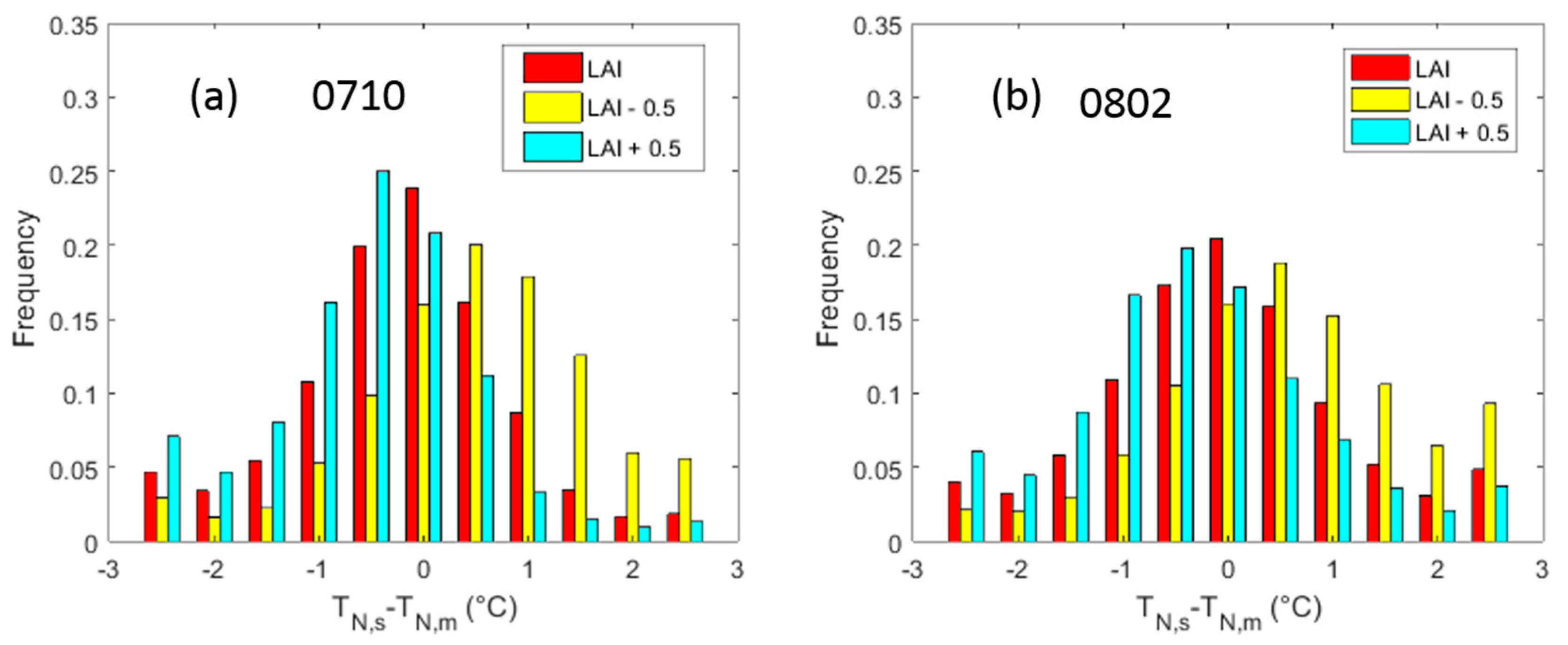
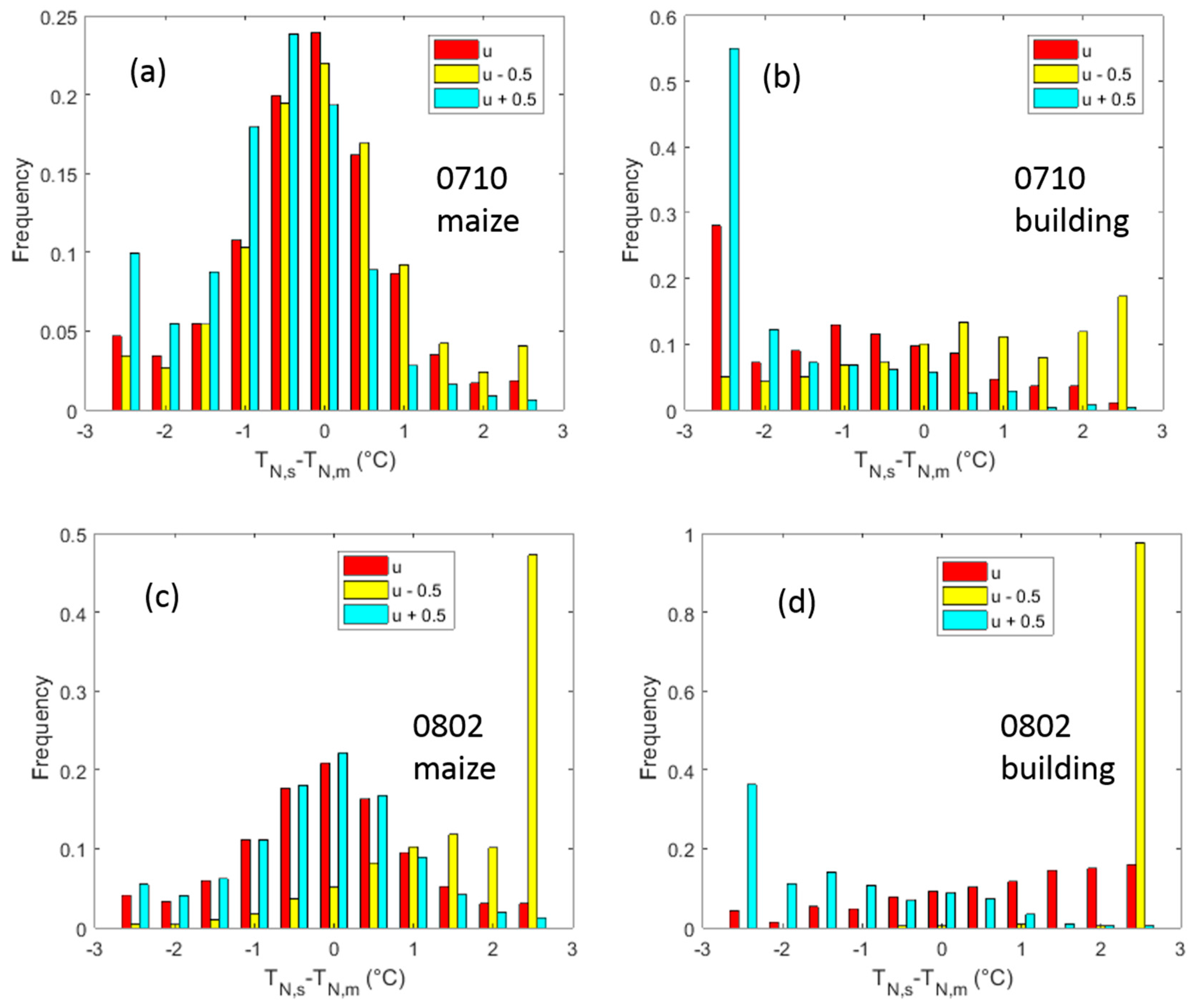
3.4. Sensitivity to the LAI and Wind Speed

During the evaluation process, errors due to input parameters are inevitable. To understand the sensitivity of the combined model to its input parameters would be very useful in order to avoid significant differences due to small errors in input parameters. A comparison of the BT and LAI images corresponding to 10 July 2012 showed that the spatial distributions of these parameters agree with each other mainly because the same height and LAD were assumed for all of the maize canopies. Therefore, the spatial distribution of the BTs simulated for the vegetation pixels was predominantly affected by their LAI values. Moreover, atmospheric fluctuations were also important factors for the simulated results because meteorological conditions averaged over a 10-minute period were used in the model while the observed BTs simply corresponded to an instantaneous state. Therefore, discrepancies between the simulated and observed results may appear. In this paper, the combined model was then analyzed by using different LAI and wind speed values and by introducing specific errors. In this analysis, the error in the LAI was set to 0.5 m/s and the error in the wind speed was set to 0.5 m/s. Four cases with different parametric errors (LAI ± 0.5 and u ± 0.5) were generated. The analysis for the LAI was performed only over vegetation pixels. When the LAI was less than 0, this value was set to 0. This sensitivity analysis was only performed with the simulated and observed BTs at 11.32 μ m .
Figure 7 displays histograms of the differences in temperature between the simulated and observed pixels with different LAI errors. The corresponding statistics can be found in Table 3. According to bias, an underestimation of the LAI value can result in simulated results that overestimate the actual values and vice versa. Compared to the results with LAI errors, the simulated results without LAI errors displayed slightly better agreement with the observations. It is inferred that no large (>0.5) discrepancies appeared in the estimated LAI values. Despite the large differences in the bias, slight differences appeared in the RMSE. To some extent, the low sensitivity to the LAI may have been related to high LAI values that occurred during the evaluation period.
Figure 8 displays histograms of the differences in temperature between the simulated and observed values with different wind speed errors. In this analysis, vegetation pixels and building pixels are evaluated separately. The evaluation results related to building pixels were significantly worse than those for vegetation pixels. According to the bias, an overestimation of the wind speed can result in simulated results that underestimate the actual values. In addition, the building pixels display a high sensitivity to the wind speed when compared to the vegetation pixels. When errors in the wind speed were induced, obvious discrepancies appeared, which is shown by the peaks on both sides of the histograms. Moreover, the underestimation of the wind speed on 2 August 2012 showed a larger impact on the simulated results than those on 10 July 2012 when the vegetation and building pixels were both significantly affected. These observations can be explained by the difference in wind speed between the two days. The value for 10 July 2012 was 1.62 m/s while the corresponding value for 2 August 2012 was 0.90 m/s. These results demonstrate that the effects of wind speed errors were not accurately reflected by their absolute values and the wind speed state should also be considered. Based on a detailed analysis of the histograms, the wind speed used for 10 July 2012 may be overestimated.
Note that the other parameters also had a strong effect on the simulated values such as the maximal carboxylation capacity [55]. Duffour et al. found that surface BTs display lower sensitivity to the maximal carboxylation capacity compared to surface heat fluxes [53]. Therefore, the empirical values are directly used for practical applications rather than obtaining them from a calibration procedure when using measured heat fluxes.

4. Discussion

4.1. Validation Issues

The validation of LSTs is still a difficult task due to the high sensitivity of this variable to atmospheric stability and the sun’s location [8,56]. In this paper, an artificial oasis over flat terrain was selected as a study area. In the evaluation process, observed ASTER TIR data were used to test the model’s performance in reconstructing the spatial distribution of surface BTs. The discrepancies shown in Figure 6 may arise because several simplifications were adopted in practical applications. In this paper, we assumed that the heights and optical properties of all of the buildings were the same, but the actual values may vary substantially across the study area. Therefore, in contrast to the observed building pixels, which displayed substantial variation, relatively similar values were simulated by the model. Moreover, the assumption of simplifying each building to a cube also leads to degradation of the simulated results. Since the RAPID-EB model is mainly used for vegetation canopies, buildings were not fully considered in the current version. Further refinement is required in the future. The results obtained for the mixed pixels that appeared between the surface types may be affected by the misclassification of land cover types. In addition, even though different vegetation types existed within the study area, they were all treated as maize canopies. These simplifications represented a practical approach, but the simulated results were affected. In spite of these discrepancies, the performance of the RAPID-EB model was acceptable. A reasonable inference is that, if more detailed surface data were used, the simulated results would be improved.
In this paper, the performance of the RAPID-EB model when reproducing spatial distributions is evaluated. Similarly, to TRGM-EB [27], the RAPID-EB model could reproduce the temporal variability in surface emissions in principle. However, the lack of long-term measured LSTs complicates this evaluation. A simple example is provided in this part using net radiation values measured at the Daman Super Station. LAI values of 4.4 and 4.2 were measured near the Daman Super Station on 10 July 2012 and 2 August 2012, respectively. Figure 9 displays scatterplots that show the relationship between the simulated and measured net radiation values on 10 July 2012 and 2 August 2012. In total, 144 pairs of measurement were used per day given the 10-minute time step. The simulated net radiation values agreed well with those measured on both 10 July 2012 and 2 August 2012 with RMSE values less than 14.0 W/m2 and R2 values greater than 0.99. One point shown in Figure 9 exhibits a large deviation. When the solar zenith angle is very small, a slight error in the sunlit fraction of the facets, which is shown in the denominator of Equation (3), may result in large errors in the net radiation.
In this paper, besides the evaluation, a procedure was developed to apply the RAPID-EB model using fine-scale VNIR data and meteorological conditions measured in situ. Landier et al. [57] proposed a methodology in which the Discrete Anisotropic Radiative Transfer (DART)-EB model can be applied over urban canopies using only remote sensing data rather than in situ measurements. In this paper, because in situ measured data were also used, the applicability of the RAPID-EB model in the inversion would be limited relative to the DART-EB model. However, for many forward simulation applications, this model can be considered suitable. According to Equation (12), the directional anisotropies of BTs can also be simulated by the RAPID-EB model. A simple comparison between RAPID-EB and TRGM-EB models is provided in Figure 10. Two types of homogeneous scenes were generated for the comparison. In the TRGM-EB, there were 960 and 3840 small triangular leaf facets in scenes with an LAI of 1.0 and 4.0, respectively. In the RAPID-EB, there were 81 large porous plant facets in the scenes. The solar zenith angle was assumed to be 15°. In Figure 10, the directional anisotropies of the simulated BTs from RAPID-EB model agreed well with those from the TRGM-EB model. The RMSDs between these simulated BTs were less than 0.58 °C. For one-day simulations (144 temporal nodes at a 10-minute step), the RAPID-EB model took approximately 3.5 minutes while the TRGM-EB model required approximately 13.5 minutes for scenes with LAI = 1.0 and required approximately 60 minutes for scenes with LAI = 4.0.

4.2. Potential Applications

According to the evaluation results, the RAPID-EB model can be viewed as a tool to dynamically simulate the distributions of surface temperatures using existing observed and measured information. Several potential applications may be explored in the future.
By combining VNIR and TIR data, the light absorption and thermal distribution of plants can be simulated. This information can support analyses of the effects of meteorological conditions on the growth of vegetation. This approach can be applied to precision agriculture for a specific crop field.
Since surface temperatures are highly sensitive to environmental factors, the simulation results are of great value in developing a protocol for use in actual experiments. For instance, given the use of meteorological parameters in previous periods and a priori knowledge of the canopy structure and component properties, the simulated temperature distribution can be used as reference data for choosing the sampling number, area, and frequency. Recently, unmanned aerial vehicles (UAVs) have been widely used in remote sensing applications [58,59]. UAVs provide a means of rapidly collecting canopy structure information over large areas with the advantages of flexibility and low cost. A potential application of the RAPID-EB model can, therefore, be anticipated by combining the spatial information from a UAV and the temporal information from a portable automatic meteorological station to provide a comprehensive synthetic dataset.
This model can also be treated as a tool that can analyze observations collected over a range of temporal and spatial scales. In the validation process, the ‘true’ values for satellite-scale pixels are typically obtained via scaling from limited data measured in situ [8,60,61,62]. The RAPID-EB model can act as a platform to convert point data measured in situ to match observed pixel data. This model can, therefore, assist in understanding scale problems in remote sensing [63,64].
In addition, the RAPID-EB model can be treated as a data generator and may, therefore, be very useful in preliminary evaluations of other simple models or inversion algorithms. Although simulation discrepancies may appear, these datasets appear to be desirable for full sensitivity analyses under various conditions.

5. Conclusions

The spatial and temporal scales of LST products cannot meet the requirements of practical applications. For the global surface EB, considerable amounts of satellite TIR data have been generated with frequent revisit intervals but coarse spatial resolutions. When applying these data, the knowledge of the temperature distribution within individual pixels would be of great value for some applications that require finely resolved LSTs. In situ experiments that provide the spatial and temporal characteristics of LSTs are limited. Model-based approaches can provide detailed information on LSTs within individual pixels. However, most existing models are not spatially explicit and others are not designed for use in remote sensing studies. Therefore, in this paper, a model that combines the RAPID model and EB methods was proposed to address this need. This model can be considered to be a new version of the combination of the TRGM and EB methods.
Using fine-scale VNIR images and temporal variations in meteorological conditions, the new model can determine the distributions of temperatures within coarse-scale TIR pixels. In this paper, an artificial oasis in the middle reaches of the Heihe River basin was selected and a practical procedure was applied to simulate the surface BTs. These simulated BTs agreed well with those observed by the ASTER sensor. The corresponding RMSE values were less than 1.6 °C and the R2 values were greater than 0.70. Although many simplifications were applied to permit its use in practical applications, the evaluation results revealed that the performance of the RAPID-EB model was acceptable. In addition, the sensitivity of the model to the LAI and wind speed was analyzed by inducing specific errors. The underestimation of the LAI and wind speed can result in simulated results that overestimate the observed values. The simulated results showed that the new model was more sensitive to the wind speed than the LAI. In addition, the analysis indicated that the effects of the input parameters cannot be described by using only their absolute deviations. Instead, their actual conditions must also be considered.
The potential applications of the RAPID-EB model were also discussed. Specifically, the model can be used as a data platform by combining spatial and temporal information to dynamically model temperature distribution at specific scales or can be used as a data generator to provide reference data in support of in situ measurements and the development of simple models. In addition, the wide use of UAV techniques would promote the application of this model in TIR remote sensing in the future.

Author Contributions

B.C., Y.D., Q.X., and Q.L. convinced and designed the experiments. Z.B., H.L., B.C., and Y.D. designed the model. Z.B. analyzed the data. B.C., H.L., and Y.D. participated in the discussion. Z.B. wrote the manuscript. Y.D. contributed to the conclusion and revision.

Acknowledgments

The ground data used in this study were obtained from the HiWATER experiments and the authors thank all of the scientists, engineers, and students who participated in the HiWATER campaign. This work was supported in part by the Chinese Natural Science Foundation Project (41571359, 41671366), the Director Foundation of the Institute of Remote Sensing and Digital Earth of the Chinese Academy of Sciences (Y5SJ1300CX), the Chinese Natural Science Foundation Project (41571357, 41501366), and the National Key Research and Development Program of China (2018YFA0605500).

Conflicts of Interest

The authors declare no conflict of interest.

References

  1. Li, Z.L.; Tang, B.H.; Wu, H.; Ren, H.; Yan, G.; Wan, Z.; Trigo, I.F.; Sobrino, J.A. Satellite-derived land surface temperature: Current status and perspectives. Remote Sens. Environ. 2013, 131, 14–37. [Google Scholar] [CrossRef]
  2. Norman, J.M.; Kustas, W.P.; Humes, K.S. Source approach for estimating soil and vegetation energy fluxes in observations of directional radiometric surface temperature. Agric. For. Meteorol. 1995, 77, 263–293. [Google Scholar] [CrossRef]
  3. Gillespie, A.; Rokugawa, S.; Matsunaga, T.; Cothern, J.S.; Hook, S.; Kahle, A.B. A temperature and emissivity separation algorithm for advanced spaceborne thermal emission and reflection radiometer (ASTER) images. IEEE Trans. Geosci. Remote Sens. 1998, 36, 1113–1126. [Google Scholar] [CrossRef]
  4. Wan, Z.; Li, Z.-L. A physics-based algorithm for retrieving land-surface emissivity and temperature from eos/modis data. IEEE Trans. Geosci. Remote Sens. 1997, 35, 980–996. [Google Scholar]
  5. Wan, Z.; Dozier, J. A generalized split-window algorithm for retrieving land-surface temperature from space. IEEE Trans. Geosci. Remote Sens. 1996, 34, 892–905. [Google Scholar]
  6. Masiello, G.; Serio, C.; De Feis, I.; Amoroso, M.; Venafra, S.; Trigo, I.F.; Watts, P. Kalman filter physical retrieval of surface emissivity and temperature from geostationary infrared radiances. Atmos. Meas. Tech. Dis. 2013, 6, 3613–3634. [Google Scholar] [CrossRef]
  7. Hulley, G.C.; Hughes, C.G.; Hook, S.J. Quantifying uncertainties in land surface temperature and emissivity retrievals from aster and modis thermal infrared data. J. Geophys. Res. Atmos. 2012, 117. [Google Scholar] [CrossRef]
  8. Li, H.; Sun, D.; Yu, Y.; Wang, H.; Liu, Y.; Liu, Q.; Du, Y.; Wang, H.; Cao, B. Evaluation of the viirs and modis lst products in an arid area of northwest china. Remote Sens. Environ. 2014, 142, 111–121. [Google Scholar] [CrossRef]
  9. Yu, Y.; Tarpley, D.; Privette, J.L.; Flynn, L.E.; Xu, H.; Chen, M.; Vinnikov, K.Y.; Sun, D.; Tian, Y. Validation of goes-r satellite land surface temperature algorithm using surfrad ground measurements and statistical estimates of error properties. IEEE Trans. Geosci. Remote Sens. 2012, 50, 704–713. [Google Scholar] [CrossRef]
  10. Masiello, G.; Serio, C.; Venafra, S.; Liuzzi, G.; Göttsche, F.; Trigo, I.F.; Watts, P. Kalman filter physical retrieval of surface emissivity and temperature from seviri infrared channels: A validation and intercomparison study. Atmos. Meas. Tech. 2015, 8, 2981–2997. [Google Scholar] [CrossRef]
  11. Blasi, M.G.; Liuzzi, G.; Masiello, G.; Serio, C.; Telesca, V.; Venafra, S. Surface parameters from SEVIRI observations through a Kalman filter approach: Application and evaluation of the scheme in Southern Italy. Tethys J. Weather Clim. West. Mediterr. 2016, 13, 3–10. [Google Scholar] [CrossRef]
  12. Bian, Z.; Xiao, Q.; Cao, B.; Du, Y.; Li, H.; Wang, H.; Liu, Q.; Liu, Q. Retrieval of leaf, sunlit soil, and shaded soil component temperatures using airborne thermal infrared multiangle observations. IEEE Trans. Geosci. Remote Sens. 2016, 54, 4660–4671. [Google Scholar] [CrossRef]
  13. Kimes, D.S. Effects of vegetation canopy structure on remotely sensed canopy temperatures. Remote Sens. Environ. 1980, 10, 165–174. [Google Scholar] [CrossRef]
  14. Lagouarde, J.-P.; Moreau, P.; Irvine, M.; Bonnefond, J.-M.; Voogt, J.A.; Solliec, F. Airborne experimental measurements of the angular variations in surface temperature over urban areas: Case study of marseille (France). Remote Sens. Environ. 2004, 93, 443–462. [Google Scholar] [CrossRef]
  15. Liang, S.; Fang, H.; Chen, M.; Shuey, C.J.; Walthall, C.; Daughtry, C.; Morisette, J.; Schaaf, C.; Strahler, A. Validating modis land surface reflectance and albedo products: Methods and preliminary results. Remote Sens. Environ. 2002, 83, 149–162. [Google Scholar] [CrossRef]
  16. Peng, J.; Liu, Q.; Wen, J.; Liu, Q.; Tang, Y.; Wang, L.; Dou, B.; You, D.; Sun, C.; Zhao, X.; et al. Multi-scale validation strategy for satellite albedo products and its uncertainty analysis. Sci. China Earth Sci. 2015, 58, 573–588. [Google Scholar] [CrossRef]
  17. Duan, S.-B.; Li, Z.-L.; Tang, B.-H.; Wu, H.; Tang, R. Generation of a time-consistent land surface temperature product from modis data. Remote Sens. Environ. 2014, 140, 339–349. [Google Scholar] [CrossRef]
  18. Duan, S.-B.; Li, Z.-L.; Wang, N.; Wu, H.; Tang, B.-H. Evaluation of six land-surface diurnal temperature cycle models using clear-sky in situ and satellite data. Remote Sens. Environ. 2012, 124, 15–25. [Google Scholar] [CrossRef]
  19. Gastellu-Etchegorry, J.-P.; Demarez, V.; Pinel, V.; Zagolski, F. Modeling radiative transfer in heterogeneous 3-D vegetation canopies. Remote Sens. Environ. 1996, 58, 131–156. [Google Scholar] [CrossRef]
  20. Qin, W.; Gerstl, S.A. 3-D scene modeling of semidesert vegetation cover and its radiation regime. Remote Sens. Environ. 2000, 74, 145–162. [Google Scholar] [CrossRef]
  21. Liu, Q.H.; Huang, H.G.; Qin, W.H.; Fu, K.H.; Li, X.W. An extended 3-D radiosity-graphics combined model for studying thermal-emission directionality of crop canopy. IEEE Trans. Geosci. Remote Sens. 2007, 45, 2900–2918. [Google Scholar] [CrossRef]
  22. Widlowski, J.-L.; Mio, C.; Disney, M.; Adams, J.; Andredakis, I.; Atzberger, C.; Brennan, J.; Busetto, L.; Chelle, M.; Ceccherini, G.; et al. The fourth phase of the radiative transfer model intercomparison (RAMI) exercise: Actual canopy scenarios and conformity testing. Remote Sens. Environ. 2015, 169, 418–437. [Google Scholar] [CrossRef]
  23. Bhumralkar, C.M. Numerical experiments on the computation of ground surface temperature in an atmospheric general circulation model. J. Appl. Meteorol. 1975, 14, 1246–1258. [Google Scholar] [CrossRef]
  24. Norman, J. Modeling the complete crop canopy. In Modification of the Aerial Environment of Plants; American Society of Agricultural Engineers: St. Joseph, MI, USA, 1979; pp. 249–280. [Google Scholar]
  25. Tol, V.D.C.; Verhoef, W.; Timmermans, J.; Verhoef, A.; Su, Z. An integrated model of soil-canopy spectral radiances, photosynthesis, fluorescence, temperature and energy balance. Biogeosciences 2009, 6, 3109–3129. [Google Scholar]
  26. Smith, J.A.; Ballard, J.R.; Pedelty, J.A. Effect of three-dimensional canopy architecture on thermal infrared exitance. Opt. Eng. 1997, 36, 3093–3100. [Google Scholar]
  27. Bian, Z.; Du, Y.; Li, H.; Cao, B.; Huang, H.; Xiao, Q.; Liu, Q. Modeling the temporal variability of thermal emissions from row-planted scenes using a radiosity and energy budget method. IEEE Trans. Geosci. Remote Sens. 2017, 55, 6010–6026. [Google Scholar] [CrossRef]
  28. Huang, H.; Qin, W.; Liu, Q. Rapid: A radiosity applicable to porous individual objects for directional reflectance over complex vegetated scenes. Remote Sens. Environ. 2013, 132, 221–237. [Google Scholar] [CrossRef]
  29. Bhumralkar, C.M. Numerical Experiments on the Computation of Ground Surface Temperature in an Atmospheric Circulation Model; DTIC Document: Dayton, OH, USA, 1974. [Google Scholar]
  30. Wallace, J.; Verhoef, A. Modelling interactions in mixed-plant communities: Light, water and carbon dioxide. Leaf Dev. Canopy Growth 2000, 204, 250. [Google Scholar]
  31. Oliphant, A.J.; Grimmond, C.S.B.; Zutter, H.N.; Schmid, H.P.; Su, H.B.; Scott, S.L.; Offerle, B.; Randolph, J.C.; Ehman, J. Heat storage and energy balance fluxes for a temperate deciduous forest. Agric. For. Meteorol. 2004, 126, 185–201. [Google Scholar] [CrossRef]
  32. Masson, V. A physically-based scheme for the urban energy budget in atmospheric models. Bound. Layer Meteorol. 2000, 94, 357–397. [Google Scholar] [CrossRef]
  33. Martilli, A.; Clappier, A.; Rotach, M.W. An urban surface exchange parameterisation for mesoscale models. Bound. Layer Meteorol. 2002, 104, 261–304. [Google Scholar] [CrossRef]
  34. Lemonsu, A.; Masson, V.; Shashua-Bar, L.; Erell, E.; Pearlmutter, D. Inclusion of vegetation in the town energy balance model for modelling urban green areas. Geosci. Model Dev. 2012, 5, 1377–1393. [Google Scholar] [CrossRef]
  35. Kanda, M.; Inagaki, A.; Miyamoto, T.; Gryschka, M.; Raasch, S. A new aerodynamic parametrization for real urban surfaces. Bound. Layer Meteorol. 2013, 148, 357–377. [Google Scholar] [CrossRef]
  36. Grimmond, C.S.B.; Oke, T.R. Aerodynamic properties of urban areas derived from analysis of surface form. J. Appl. Meteorol. 1999, 38, 1262–1292. [Google Scholar] [CrossRef]
  37. Huang, H. Rapid2: A 3D simulator supporting virtual remote sensing experiments. In Proceedings of the 2016 IEEE International Geoscience and Remote Sensing Symposium (IGARSS), Beijing, China, 10–15 July 2016; pp. 3636–3639. [Google Scholar]
  38. Farquhar, G.V.; von Caemmerer, S.V.; Berry, J. A biochemical model of photosynthetic CO2 assimilation in leaves of C3 species. Planta 1980, 149, 78–90. [Google Scholar] [CrossRef] [PubMed]
  39. Collatz, G.J.; Ribas-Carbo, M.; Berry, J. Coupled photosynthesis-stomatal conductance model for leaves of C4 plants. Funct. Plant Biol. 1992, 19, 519–538. [Google Scholar]
  40. Olioso, A.; Chauki, H.; Bergaoui, K.; Bertuzzi, P.; Chanzy, A.; Bessemoulin, P.; Clavet, J.-C. Estimation of energy fluxes from thermal infrared, spectral reflectances, microwave data and svat modeling. Phys. Chem. Earth Part B Hydrol. Oceans Atmos. 1999, 24, 829–836. [Google Scholar] [CrossRef]
  41. Wang, H.; Xiao, Q.; Li, H.; Du, Y.; Liu, Q. Investigating the impact of soil moisture on thermal infrared emissivity using aster data. IEEE Geosci. Remote Sens. Lett. 2015, 12, 294–298. [Google Scholar] [CrossRef]
  42. Berk, A.; Anderson, G.P.; Bernstein, L.S.; Acharya, P.K.; Dothe, H.; Matthew, M.W.; Adler-Golden, S.M.; Chetwynd, J.H., Jr.; Richtsmeier, S.C.; Pukall, B. Modtran 4 radiative transfer modeling for atmospheric correction. In Proceedings of the SPIE- The International Society for Optical Engineering, Denver, CO, USA, 20 October 1999; pp. 348–353. [Google Scholar]
  43. Li, X.; Cheng, G.; Liu, S.; Xiao, Q.; Ma, M.; Jin, R.; Che, T.; Liu, Q.; Wang, W.; Qi, Y. Heihe watershed allied telemetry experimental research (hiwater): Scientific objectives and experimental design. Bull. Am. Meteorol. Soc. 2013, 94, 1145–1160. [Google Scholar] [CrossRef]
  44. Xu, Z.; Liu, S.; Li, X.; Shi, S.; Wang, J.; Zhu, Z.; Xu, T.; Wang, W.; Ma, M. Intercomparison of surface energy flux measurement systems used during the hiwater-musoexe. J. Geophys. Res. Atmos. 2013, 118, 13140–13157. [Google Scholar] [CrossRef]
  45. Song, L.; Liu, S.; Zhang, X.; Zhou, J.; Li, M. Estimating and validating soil evaporation and crop transpiration during the hiwater-musoexe. IEEE Geosci. Remote Sens. Lett. 2015, 12, 334–338. [Google Scholar] [CrossRef]
  46. Zhong, B.; Peng, M.A.; Nie, A.H.; Yang, A.X.; Yao, Y.J.; Wenbo, L.; Zhang, H.; Liu, Q.H. Land cover mapping using time series HJ-1/CCD data. Sci. China Earth Sci. 2014, 57, 1790–1799. [Google Scholar] [CrossRef]
  47. Zhong, B.; Yang, A.; Nie, A.; Yao, Y.; Zhang, H.; Wu, S.; Liu, Q. Finer resolution land-cover mapping using multiple classifiers and multisource remotely sensed data in the heihe river basin. IEEE J. Sel. Top. Appl. Earth Obs. Remote Sens. 2015, 8, 4973–4992. [Google Scholar] [CrossRef]
  48. Li, Y.; Huang, C.; Hou, J.; Gu, J.; Zhu, G.; Li, X. Mapping daily evapotranspiration based on spatiotemporal fusion of aster and modis images over irrigated agricultural areas in the heihe river basin, northwest china. Agric. For. Meteorol. 2017, 244, 82–97. [Google Scholar] [CrossRef]
  49. Jacquemoud, S.; Baret, F. Prospect: A model of leaf optical properties spectra. Remote Sens. Environ. 1990, 34, 75–91. [Google Scholar] [CrossRef]
  50. Baldridge, A.M.; Hook, S.J.; Grove, C.I.; Rivera, G. The aster spectral library version 2.0. Remote Sens. Environ. 2009, 113, 711–715. [Google Scholar] [CrossRef]
  51. Borel, C.C. Surface emissivity and temperature retrieval for a hyperspectral sensor. In Proceedings of the 1998 IEEE International Geoscience and Remote Sensing Symposium Proceedings, Seattle, WA, USA, 6–10 July 1998; pp. 546–549. [Google Scholar]
  52. Yamaguchi, Y.; Kahle, A.B.; Tsu, H.; Kawakami, T.; Pniel, M. Overview of advanced spaceborne thermal emission and reflection radiometer (ASTER). IEEE Trans. Geosci. Remote Sens. 1998, 36, 1062–1071. [Google Scholar] [CrossRef]
  53. Duffour, C.; Olioso, A.; Demarty, J.; Van der Tol, C.; Lagouarde, J.-P. An evaluation of scope: A tool to simulate the directional anisotropy of satellite-measured surface temperatures. Remote Sens. Environ. 2015, 158, 362–375. [Google Scholar] [CrossRef]
  54. Yang, K.; Wang, J. A temperature prediction-correction method for estimating surface soil heat flux from soil temperature and moisture data. Sci. China Ser. D Earth Sci. 2008, 51, 721–729. [Google Scholar] [CrossRef]
  55. Cowan, I. Stomatal behaviour and environment. Adv. Bot. Res. 1977, 4, 117–128. [Google Scholar]
  56. Lagouarde, J.-P.; Irvine, M.; Dupont, S. Atmospheric turbulence induced errors on measurements of surface temperature from space. Remote Sens. Environ. 2015, 168, 40–53. [Google Scholar] [CrossRef]
  57. Landier, L.; Lauret, N.; Yin, T.; Bitar, A.A.; Gastellu-Etchegorry, J.; Feigenwinter, C.; Parlow, E.; Mitraka, Z.; Chrysoulakis, N. Remote sensing studies of urban canopies: 3D radiative transfer modeling. In Sustainable Urbanization; Ergen, M., Ed.; InTech: Rijeka, Croatia, 2016; p. 10. [Google Scholar]
  58. Everaerts, J. The use of unmanned aerial vehicles (UAVS) for remote sensing and mapping. Int. Arch. Photogramm. Remote Sens. Spat. Inf. Sci. 2008, 37, 1187–1192. [Google Scholar]
  59. Colomina, I.; Molina, P. Unmanned aerial systems for photogrammetry and remote sensing: A review. ISPRS J. Photogramm. Remote Sens. 2014, 92, 79–97. [Google Scholar] [CrossRef]
  60. Liu, S.; Xu, Z.; Song, L.; Zhao, Q.; Ge, Y.; Xu, T.; Ma, Y.; Zhu, Z.; Jia, Z.; Zhang, F. Upscaling evapotranspiration measurements from multi-site to the satellite pixel scale over heterogeneous land surfaces. Agric. For. Meteorol. 2016, 230, 97–113. [Google Scholar] [CrossRef]
  61. Wu, X.; Wen, J.; Xiao, Q.; Liu, Q.; Peng, J.; Dou, B.; Li, X.; You, D.; Tang, Y.; Liu, Q. Coarse scale in situ albedo observations over heterogeneous snow-free land surfaces and validation strategy: A case of modis albedo products preliminary validation over northern china. Remote Sens. Environ. 2016, 184, 25–39. [Google Scholar] [CrossRef]
  62. Hulley, G.C.; Hook, S.J. Generating consistent land surface temperature and emissivity products between aster and modis data for earth science research. IEEE Trans. Geosci. Remote Sens. 2011, 49, 1304–1315. [Google Scholar] [CrossRef]
  63. Li, X.; Strahler, A.H.; Friedl, M.A. A conceptual model for effective directional emissivity from nonisothermal surfaces. IEEE Trans. Geosci. Remote Sens. 1999, 37, 2508–2517. [Google Scholar]
  64. Li, X.; Wang, J.; Strahler, A. Scale effects and scaling-up by geometric-optical model. In Proceedings of the IEEE 1999 International Geoscience and Remote Sensing Symposium, Hamburg, Germany, 28 June–2 July 1999; pp. 1875–1877. [Google Scholar]
Figure 1. (a) Actual forest canopy and (b) illumination of plant objects. Horizontally arranged green facets are used to represent groups of small leaf facets in each layer and yellow facets are used to represent trunks.
Remotesensing 10 00736 g001
Figure 2. The scheme used to test the RAPID-EB model over the study area in this paper. The data preparation steps are indicated in green, the RAPID-EB model and its outputs are indicated in yellow, and the test steps are indicated in blue.
Remotesensing 10 00736 g002
Figure 3. The location of the study area. The green circles represent automatic meteorological stations. The background shows an ASTER false-color VNIR image of the study area taken on 10 July 2012.
Remotesensing 10 00736 g003
Figure 4. Distribution of LAI values within the study area on (a) 10 July 2012 and (b) 2 August 2012.
Remotesensing 10 00736 g004
Figure 5. Ground photograph of (a) the Daman Super Station located at 100°22′ E, 38°51′ N and the spatial distribution of the 0–5 cm soil moisture over the study area as a whole on (b) 10 July 2012 and (c) 2 August 2012. 0710 stands for 10 July 2012 while 0802 stands for 2 August 2012.
Remotesensing 10 00736 g005
Figure 6. Observed (a,b) and simulated (c,d) surface BTs at 11.32 μm on two days (10 July 2012 and 2 August 2012) and the corresponding scatterplots (e,f). The solid line represents the 1:1 line while the dotted lines represent the 1:1 line ± the RMSE. All of the BTs are given in °C.
Remotesensing 10 00736 g006
Figure 7. Histograms of the differences in temperature between the simulated and observed values with different LAI errors correspond to (a) 10 July 2012 and (b) 2 August 2012.
Remotesensing 10 00736 g007
Figure 8. Histograms of the differences in temperature between the simulated and observed values with different wind speed errors on (a,b) 10 July 2012 and (c,d) 2 August 2012. (a,c) refer to vegetation pixels, and (b,d) refer to building pixels.
Remotesensing 10 00736 g008
Figure 9. Scatterplots showing the relationship between the simulated and measured net radiation on (a) 10 July 2012 and (b) 2 August 2012. In total, 144 pairs of measurements were used for each day.
Remotesensing 10 00736 g009
Figure 10. The comparison of BTs simulated by TRGM-EB and RAPID-EB models in the solar principle plane. The black and white points represent scenes with LAI = 1.0 and LAI = 4.0, respectively. The solar zenith angle was assumed to be 15°.
Remotesensing 10 00736 g010
Table 1. Leaf parameters used in the PROSPECT model and the emissivities of the components in the ASTER bands.
ParameterLeaf (Maize)SoilWallRoof
N1.518---
Cab (µg/cm²)58---
Cw (g/cm²)0.013---
Cm (g/cm²)0.003662---
Emissivity Band 10
(8.29 μ m )
0.9820.9400.9830.909
Emissivity Band 11
(8.63 μ m )
0.9830.9520.9460.887
Emissivity Band 12
(9.07 μ m )
0.9760.9470.8690.870
Emissivity Band 13
(10.66 μ m )
0.9680.9720.8850.912
Emissivity Band 14
(11.32 μ m )
0.9790.9750.8950.923
N: leaf structure parameter; Cab: chlorophyll content. Cw: equivalent water thickness; Cm: dry matter content.
Table 2. Statistical information on the simulated BTs over the study area for each band.
Band 10Band 11Band 12Band 13Band 14
DateR2RMSE (°C)R2RMSE (°C)R2RMSE (°C)R2RMSE (°C)R2RMSE (°C)
07100.761.340.741.410.701.520.741.440.751.33
08020.721.580.731.450.721.370.731.510.731.55
Table 3. Statistical information on the simulated BTs with different LAI and wind speed errors.
AllMaizeBuilding
CaseRMSE (°C)Bias (°C)RMSE (°C) Bias (°C) RMSE (°C) Bias (°C)
0710---1.33−0.281.14−0.192.11−1.16
LAI − 0.5 1.360.48
LAI + 0.5 1.26−0.54
u − 0.51.340.011.21−0.021.890.66
u + 0.51.69−0.901.41−0.733.15−2.52
0802---1.290.011.20−0.081.730.78
LAI − 0.5 1.460.57
LAI + 0.5 1.37−0.33
u − 0.54.103.093.452.547.937.73
u + 0.51.37−0.291.19−0.242.42−1.73

