A Smart MCDM Framework to Evaluate the Impact of Air Pollution on City Sustainability: A Case Study from China

Abstract

Air pollution has become one of the key environmental concerns in the urban sustainable development. It is important to evaluate the impact of air pollution on socioeconomic development since it is the prerequisite to enforce an effective prevention policy of air pollution. In this paper, we model the impact of air pollution on the urban economic development as a Multiple Criteria Decision Making (MCDM) problem. In particular, we propose a novel Technique for Order of Preference by Similarity to Ideal Solution (TOPSIS) analysis framework to evaluate multiple factors of air pollutants and economic development. Our method can overcome the drawbacks of conventional TOPSIS methods by using Bayesian regularization and the Back-Propagation (BP) neural network to optimize the weight training process. We have conducted a case study to evaluate our proposed framework.

1. Introduction

Air pollution has become one of the most important environment problems, which can significantly affect the sustainable urban development. In particular, atmospheric pollutants not only are harmful to health [1,2,3,4], but also can cause substantial economic loss [5], especially in many developing countries. For example, it is shown in [6] that the economic loss due to air pollution in China in 2010 reached 1.1 trillion (1 trillion = ${10}^{12}$) yuan, accounting for 13.7% of the total Gross Domestic Product (GDP) of that year. Therefore, the prevention or control of air pollution has become a top issue in socioeconomic development.

However, the policy of prevention or control of air pollution in developing counties has usually lagged behind the socioeconomic development. As a result, ambient air quality has deteriorated significantly. Air pollution is mainly due to the air pollutant emissions [7,8,9], the rapid urban growth [10] and the shrinking green space [11]. Recently, a number of control technologies on air pollution have been proposed and developed [12]. One of the most important prerequisites of the effective prevention of air pollution lies in the evaluation of air pollution on socioeconomic development.

A number of efforts have been put into evaluating the impact of air pollution on economic development [13,14,15,16,17,18]. Most of these studies are mainly based on the evaluation of domain experts or government officers. However, the evaluation results are often affected by the knowledge, experience and the emotional state of the experts or officers. As a result, the evaluation results are often biased or subjective and cannot accurately reflect the real impact of air pollution. Therefore, it is necessary to propose an accurate and objective evaluation framework to investigate the impact of air pollution on the economic development.

The air quality is often affected by many factors, which fluctuates from time to time. For example, Figure 1 shows that Air Quality Index (AQI) varies with air pollution indicators (such as SO${}_2$, NO${}_2$, PM${}_{10}$, dustfall and pH) in Wuhan City in China from 1996 to 2016. Essentially, air pollution is a result of multi-factor interaction in the complex atmosphere system. There are multiple pollutants affecting the air quality [19]. Thus, the evaluation of air pollution and the economic development can be regarded as a Multiple Criteria Decision Making (MCDM) problem that involves many conflicting evaluation indicators, such as various air pollutants, AQI and GDP per capital.

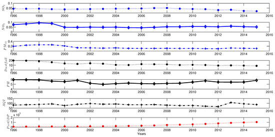
Figure 1. Indicators of air pollution and GDP from 1995 to 2015.

The Technique for Order of Preference by Similarity to Ideal Solution (TOPSIS) [20,21] is a kind of MCDM method. Compared with other MCDM methods, such as fuzzy-set theory [22,23] and the Analytic Hierarchy Process (AHP) [24], TOPSIS has many merits such as the simplicity and insensitivity to the number of alternatives (or indicators) [25]. However, TOPSIS has difficulties in determining the weights of multiple alternatives and keeping the consistency of judgment [26]. For example, most of the TOPSIS methods require the weight evaluations given by domain experts [27]; this inevitably leads to the bias in the evaluation and the subjective decision [28]. Besides, most of studies on TOPSIS are mainly focused on business decision making problems [29,30]. To the best of our knowledge, there are few studies on the evaluation of the impact of air pollution on economic development by using the TOPSIS method.

In this paper, we propose a novel TOPSIS-based MCDM method (named the Smart MCDM) to evaluate the impact of air pollution on the economic development. The primary research contributions of this paper can be summarized as follows:

• We propose the entropy method to obtain the initial weights of indicators of air pollution. This method can overcome the disadvantages of conventional TOPSIS methods in determining initial weights (recall that conventional methods obtain the weights given by domain experts).
• Besides, we integrate Bayesian regularization and the Back-Propagation (BP) neural network in our Smart MCDM framework in order to obtain the objective weights since there is a correlation between the weights. The benefit of using Bayesian regularization in the BP neural network lies in the performance improvement in training the weights.
• Moreover, we have applied Smart MCDM to evaluate the impact of air pollution on the economic development of Wuhan City in China. The empirical study is conducted on data collected from 1996 to 2015, focusing on seven indicators (including six major air pollution indicators and one economic indicator). The empirical results not only validate the effectiveness of our proposed MCDM framework, but also provide many implications on balancing the economic development and environment protection.

The rest of the paper is organized as follows. Section 2 presents the Smart MCDM framework. We then present a case study in Section 3. Section 4 concludes the paper.

2. Smart MCDM Framework

In order to address the aforementioned concerns, we propose a Smart MCDM framework based on TOPSIS. As shown in Figure 2, our framework consists of four key phases: feature transformation (as shown in Section 2.1), feature selection (as shown in Section 2.2), weight training (as shown in Section 2.3) and evaluation (as shown in Section 2.4). We then describe them in detail as follows.

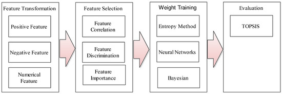
Figure 2. Our proposed Multiple Criteria Decision Making (MCDM) framework.

2.1. Feature Transformation

Since the indicators (also named as features interchangeably throughout the whole paper) of air pollutants are in different units, we need to normalize them before conducting feature selection. In particular, we convert the absolute value of an indicator into the relative one. Moreover, the positive indicator value and the negative indicator value represent different meanings. For example, air pollution is the negative indicator, while GDP is the positive indicator. Therefore, we choose the MAX-MIN scaling method to normalize the positive and negative values. More specifically, we have:

• Positive values:

  $$x_{ij}=\frac{u_{ij}-min(u_{ij})}{max(u_{ij})-min(u_{ij})},$$

  (1)
• Negative values:

  $$x_{ij}=\frac{max(u_{ij})-u_{ij}}{max(u_{ij})-min(u_{ij})},$$

  (2)

  where $u_{ij}$ represents the original value, $x_{ij}$ represents the value after normalization, $min(·)$ is the minimum value and $max(·)$ is the maximum value.

2.2. Feature Selection

Air pollution is a result of multi-factor interaction in the Earth’s complex atmosphere. There are multiple pollutants having an influence on air pollution. To simplify our analysis, we need to identify several major pollutants that have a significant impact on urban air pollution [31]. In this paper, we mainly consider the following major air pollutants according to China ambient air quality standards (i.e., GB3095-2012 standard [32]): sulfur dioxide (SO${}_2$), nitrogen dioxide (NO${}_2$), Particulate Matter with a diameter of 10 $\mathsf{\mu }$m or less (PM${}_{10}$) and particulate matter with a diameter of 2.5 $\mathsf{\mu }$m or less (PM${}_{2.5}$). It is worth mentioning that PM${}_{2.5}$ has been considered only after 1 January 2016 when China’s new ambient air quality standard came into force (though Wuhan City released the four-year data of PM${}_{2.5}$ from 2012 to 2016 since it is one of the experimental cities in China). Since most of the information of PM${}_{2.5}$ is missing for the years from 1996 to 2015, we do not consider PM${}_{2.5}$ in this paper.

2.3. Weight Training

Figure 3 shows the weight training procedure. In particular, we first use the entropy method to obtain the initial weights for the indicators, as shown in Section 2.3.1. In order to solve the correlation of initial weights, we then use Back-Propagation (BP) neural networks to train the weights, as shown in Section 2.3.2.

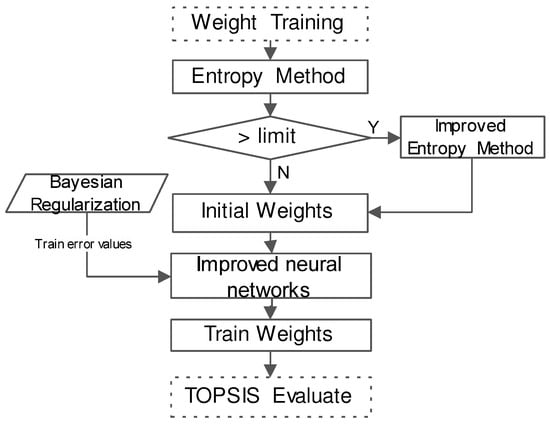
Figure 3. Weight training procedure.

2.3.1. Entropy Method to Determine Initial Weights

In information theory, entropy is a measure of uncertainty [33]. In this paper, we use the entropy method [27] to determine the weights of the indicators. In particular, we have the following equation to calculate the entropy denoted by $H(\chi )$ of information $\chi$:

$$H(\chi )=-\sum _{i=1}^{m}P({\chi }_i)\ln P({\chi }_i),$$

(3)

where ${\chi }_i$ is the i-th value (there are in total m states) and $P({\chi }_i)$ is the probability of the i-th state.

The entropy can be used to evaluate the randomness and the disorder degree of an event (or an indicator). In other words, the bigger the indicator is, the higher the influence on the comprehensive evaluation, implying smaller entropy. In this paper, we select m data samples and n indicators for evaluation, which construct a matrix $X={(x_{ij})}_{m\times n}$.

We propose Algorithm 1 to generate the initial weights. The main idea of Algorithm 1 can be summarized as the following steps.

• Normalization of indicators: Since the indicators of air pollutants are in different units, we need to normalize them first. In particular, we can use the feature transformation method in Section 2.1 to solve this issue.
• Calculation of the entropy measure: We then calculate the entropy measure of the i-th sample under indicator j (j is ranging from one to n) by the following equation:

  $$\begin{array}{c}\hfill e_j=-k·{\displaystyle \sum _{i=1}^m}p(x_{ij})·\ln p(x_{ij}),\end{array}$$

  (4)

  where k is the proportional parameter [34]. If we choose $e_j\in [0,1]$, then $k={(\ln m)}^{-1}$ [27].
  We next have $h_j=1-e_j$ from Equation (4).
• Calculation of the entropy weight: We then calculate the entropy weight of each j as follows,

  $$w_j=\frac{h_j}{{\sum }_{j=1}^n{h}_j}.$$

  (5)
• Calculation of redundancy (weight correction): When any element $w_j$ needs to be corrected (i.e., $w_j>0.25$), we first correct the weight as $w_k^{*}=0.25$. Then, the remaining part of $w_k-0.25$ will be assigned to other $m-1$ weights proportionally according to the following equation:

  $$w_j^{*}=w_j+\frac{w_k}{{\sum }_{j=1}^n{w}_j}·(w_k-0.25),$$

  (6)

  where k is the index of the element that needs to be corrected and $j\ne k$. We then obtain the corrected entropy weight $W^{*}=(w_1^{*},w_2^{*},w_3^{*},\dots ,w_n^{*})$. If any weight in $W^{*}$ needs the correction again (i.e., $W_k^{*}>0.25$), we repeat the above steps until no more corrections are need.

Algorithm 1 Improved entropy weight method.

1: $k:=1/\ln (m)$ 2: for $j:=1$ to n do 3:   calculate each $e_j:=-k·{\sum }_{i=1}^{m}p(x_{ij})·\ln p(x_{ij})$ 4: end for 5: $h_j:=1-e_j$ 6: $w_j:=h_j/{\sum }_{j=1}^n(h_j)$ 7: while $w_j^{*}>0.25$ do 8:   correct the n weights according to Equation (6). 9: end while

2.3.2. Integration of Bayesian Regularization and BP Neural Networks to Train Weights

Although the entropy method is an objective evaluation method to obtain the initial weights, there is a correlation between the weights. In order to obtain objective weights, we introduce the Back-Propagation (BP) neural network to train initial weights obtained by the aforementioned entropy method. Since the parameters of the neural networks are generally selected according to experiential knowledge (resulting in the local optimum [35]), we use Bayesian regularization to improve the training procedure of BP neural networks. Before the formal introduction of our method, we firstly briefly review the Artificial Neural Network (ANN) as follows.

Artificial Neural Network

ANN [35] was proposed to simulate the intelligent process of the human brain. ANN is mainly composed of artificial neurons, the ANN learning model and network topology. Figure 4 depicts a neural network training procedure. In particular, there are four basic elements in ANN:

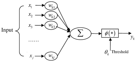
Figure 4. Neural network training procedure.

• A set of neurons (corresponding to the synapses of biological neurons).
• A unit to calculate the weighted sum (linear combination) of the input signals.
• A non-linear activation function.
• A threshold ${\theta }_k$.

More specifically, we can represent the above process as the following equation:

$$u_k=\sum _{j=1}^n{w}_{kj}{x}_j,v_k=u_k-{\theta }_k,y_k=\varphi (v_k),$$

(7)

where $x_1,x_2,x_3,\dots ,x_n$ are input signals, $w_{k1},w_{k2},w_{k3},\dots ,w_{kn}$ are weights of neurons, $v_k$ is the value of neural networks, $u_k$ is the linear combination, ${\theta }_k$ is the threshold, $\varphi (\ast )$ is activation function and $y_k$ is the output.

Training Parameter Selection on the BP Neural Network

The BP neural network is a nonlinear general transformation unit composed of a feed-forward network. There are two phases in the BP neural network: propagation and weight updating. Specifically, an input vector is propagated in the layer-by-layer manner through the network until it finally reaches the output layer. A comparison between the output and the desired output is then conducted, and an error value is calculated for each neuron in the output layer. Then, the error values are propagated back to the network starting from the output to each backward layer. In this manner, each neuron is then associated with an error value (roughly representing the contribution to the original output). This process will repeat until the error reaches an acceptable level.

In this paper, the idea of training weight is to use the existing features as the input vector. We then choose the training sample set as the input sample. We next choose the initial weights as the output so that we can determine the number of layers, the number of neurons in each layer and the learning parameters. In the sample set, the factor quantization value is known (i.e., the factor score). After initialization, the network weights are obtained through network training. In order to obtain the corrected weights in features, we need to calculate the correlation between the network weights. During the process, how to choose the appropriate training parameters is a key for the efficiency of BP neural networks. We next analyze the selection of the training parameters.

• Expected error: In BP neural network training process, it is important to choose a proper value of the expected error. For example, if the expected error is too small, the same set of sample data will be used repeatedly, resulting in over-fitting, while choosing a larger value of the expected error can also lead to a larger number of training times. In general, the empirical value is 0.0001, while we choose 0.00049 by using the Bayesian regulation method (shown as follows) in this paper.
• Number of hidden nodes: In this paper, we use a method named the Trial-And-Error (TAE) method to determine the number of hidden nodes. First, we set fewer hidden nodes in the network. We then gradually increase the number of hidden nodes. When the error reaches the minimum, we then obtain the number of the hidden nodes.
• Number of layers: It is shown in [35] that the feed-forward network with a single hidden layer can map all continuous functions. It is true that increasing the number of hidden layers can reduce the training error while it can also result in the complex structure. In fact, as indicated above, increasing the number of nodes can also reduce the training error. Therefore, we choose a three-layer feed-forward network with a single hidden layer in this paper.
• Activation function: According to the characteristics of ANN approximation, the activation function of the hidden layer is sigmoidal function that can be expressed as follows,

  $$y=f(x)=\frac{1}{1+e^{-\lambda x}}.$$

  (8)

  where $\lambda$ is the modifier [35]. Without loss of generality, we choose $\lambda$ = 1 in this paper.

Bayesian Regularization Improves the BP Neural Network

One of disadvantages of the BP neural network is that the learning process is easily trapped in the local minimum resulting in poor network scalability. In this paper, we use regularization to limit the scale of network weights so that we can improve the generalization of neural networks. In particular, we consider Bayesian regularization, which is a method to estimate the regularization parameters based on Bayesian methods [36]. It is worth mentioning that there are many methods to improve or optimize the weights of the neural networks, including Genetic Algorithms (GA), Particle Swarm Optimization (PSO), etc. [37,38,39]. In this paper, we choose Bayesian regularization mainly because the data in our study are scarce, and the Bayesian method can improve the performance of neural networks (by reducing the training iterations) [36]. One of our future works is to use other methods, such as GA and PSO, to optimize the weights in neural networks.

The main idea of Bayesian regularization is described as follows: (1) we first give a set of training samples $S=(p_1,t_1),(p_2,t_3),(p_3,t_3),\dots ,(p_m,t_m)$; (2) we then find the effective approximation function to minimize the error through neural network learning process. Figure 5 depicts a Bayesian neural network training procedure. In particular, we choose the mean square sum error function defined as follows,

$$E_D=\frac{1}{n}\sum _{t=1}^n{(t_i-a_i)}^2,$$

(9)

where n is the number of samples, $t_i$ is the expected output value and $a_i=f(p_i)$ is the actual output value for the network. In order to improve the generalization ability, we can add the arithmetic average of the network weights in the objective function. We then have the objective function as follows,

$$F=\beta E_D+\alpha E_W,$$

(10)

where $E_W=\frac{1}{m}{\sum }_{i=1}^m{w}_i^2$ is the summation of the squares of the network weights, $w_i$ is the neural network connection weight, m is the number of neural network connection weights and $\alpha$ and $\beta$ are the parameters of the objective function. Bayesian regularization can adjust $\alpha$ and $\beta$ in the network training process so that it can effectively control the complexity of the network under the promise of the square sum error. In Section 3.2, we will demonstrate the significant performance improvement of Bayesian regularization neural networks over the conventional neural networks.

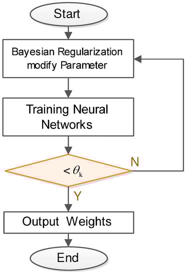
Figure 5. Bayesian training procedure.

2.4. Evaluation Based on TOPSIS

The main idea of TOPSIS is that the optimal evaluation object should have the shortest geometric distance from the positive ideal solution and the longest geometric distance from the negative ideal solution. In this paper, we use TOPSIS to evaluate the impacts of various air pollutants on the air pollution. In particular, we first use Equation (1) or Equation (2) to normalize the original datasets. More specifically, we denote $Y=\left(y_1,y_2,y_3,\dots ,y_j\right)=y_{ij}$ by the normalized matrix.

We then determine the optimal sample and the worst sample of each indicator. Specifically, the optimal sample is constructed by using the maximum value of each indicator in all samples. The minimum sample of each indicator is used to construct the worst sample. We denote the optimal sample and the worst sample by $Y^{+}$ and $Y^{-}$, respectively. More specifically, they can be represented by the following equations:

$$Y^{+}=(y_1^{+},y_2^{+},\dots ,y_n^{+}),Y^{-}=(y_1^{-},y_2^{-},\dots ,y_n^{-}),$$

(11)

where $y_j^{+}=\underset{1\le i\le m}{max}{y}_{ij}$ and $y_j^{-}=\underset{1\le i\le m}{max}{y}_{ij},j=1,2,\dots n$.

We next calculate the relative distance from each sample point to the optimal sampling point denoted by $C_i$, which can be calculated by the following equation,

$$C_i=\frac{D_i^{-}}{D_i^{+}+D_i^{-}},$$

(12)

where $D_i^{+}$ is the distance from each sample point to the optimum sample point and $D_i^{-}$ is the distance from each sample point to the worst sample point. More specifically, $D_i^{+}=\sqrt{{\sum }_{j=1}^n{(y_{ij}-y_j^{+})}^2},D_i^{-}=\sqrt{{\sum }_{j=1}^n{(y_{ij}-y_j^{-})}^2},i=1,2,\dots m$. In this paper, we mainly concentrate on the indicator of air pollution denoted by $C(\mathrm{Air}\mathrm{Pollution})$ and the joint indicator of both air pollution and GDP denoted by $C(\mathrm{Air}\mathrm{Pollution}\mathrm{and}\mathrm{GDP})$. In Section 3, we will evaluate them by using our proposed MCDM framework.

3. Case Study

We choose the sample dataset of the air pollution of Wuhan City in China [40]. This dataset has been issued by Wuhan Environmental Protection Bureau from 1996 to 2015. We select six major air pollutants according to the Chinese GB3095-2012 standard [32]. Moreover, we choose the sample dataset about the Gross Domestic Product (GDP) of Wuhan City in China from 1996 to 2015, which has been issued by the Wuhan Municipal Bureau of Statistics [41].

We apply the proposed analytical model (presented in Section 2) to evaluate the impacts of air pollution on the economic development in the case study of Wuhan City of China. It is worth mentioning that multiple criteria are imperfect and contain uncertain factors during the analysis. Thus, our proposed Smart MCDM can offer the solution to this multi-criteria problem. Figure 6 depicts the analytical process. We next describe the different phases in details.

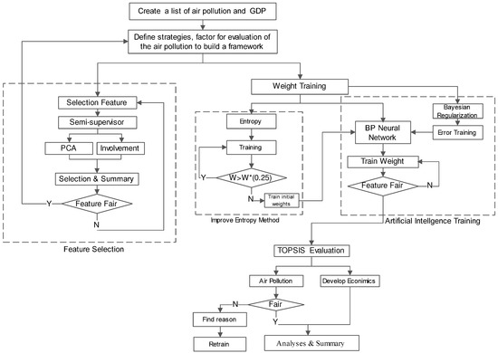
Figure 6. Analytical framework.

3.1. Feature Selection

There are six major air pollutants according to China Ambient air quality standards (i.e., GB3095-2012 standard [32]): sulfur dioxide (SO${}_2$), nitrogen dioxide (NO${}_2$), ozone (O${}_3$), carbon monoxide (CO), PM${}_{2.5}$ and PM${}_{10}$. Note that the information of PM${}_{2.5}$ is missing for the years from 1996 to 2015 since it has been considered only after 1 January 2016 when China’s new air quality standard came into force. Therefore, we do not consider PM${}_{2.5}$ in this paper. Before applying our proposed Smart MCDM model to TOPSIS evaluation, we need to quantify the importance of every indicator in the sample data. Specifically, we choose the indicators that contribute the most to our model. In this paper, we use Principal Component Analysis (PCA) [42] to extract the most influential indicators. The problem of choosing the number of components is still open as indicated in [43], though it is suggested that we should choose 5 to 10-times as many subjects as variables [44,45]. Therefore, we follow the guidelines [42,46] to analyze the accumulative variance of these air pollutants and finally choose the three most influential indicators, i.e., SO${}_2$, NO${}_2$ and PM${}_{10}$. As shown in Table 1, the three most influential indicators (SO${}_2$, NO${}_2$, PM${}_{10}$ with bold fonts) contribute to 94.319% among all of the indicators, satisfying the requirement of the guidelines according to [42,46]. In addition to the above air pollutants, there are also other air pollution indicators, such as dustfall, potential of hydrogen (pH) of precipitation and the Air Quality Index (AQI), which will be used with the above three major air pollutants to measure the air quality.

Table 1. Accumulative Variance based on the PCA method.

Indicator	Total Value	Variance (%)	Accumulative Total (%)
SO${}_2$	2.724	54.479	54.479
NO${}_2$	1.162	23.248	77.727
PM${}_{10}$	0.830	16.592	94.319
O${}_3$	0.179	3.590	97.908
CO	0.105	2.092	100.000

3.2. Weight Training

We then conduct weight training on the air pollution indicators and GDP. In particular, we first normalize the indicators according to Section 2.1. More specifically, SO${}_2$, NO${}_2$, PM${}_{10}$, dustfall and AQI are negative indicators according to Equation (2) while pH and GDP are positive indicators according to Equation (1). We next use entropy method according to Algorithm 1 to obtain the initial weights of each indicator. Table 2 presents the initial weights of the indicators from 1996 to 2015.

Table 2. Initial weights obtained by the entropy method for Air Quality Index.

Year	SO${}_2$	NO${}_2$	PM${}_{10}$	Dustfall	pH	AQI
1996	0.0346	0.0252	0.0277	0.0002	0.1003	0.0590
1997	0.0346	0.0140	0.0078	0.0023	0.0974	0.0522
1998	0.0303	0.0001	0.0004	0.0098	0.0953	0.0431
1999	0.0519	0.0084	0.0001	0.0251	0.0694	0.0317
2000	0.0606	0.0631	0.0212	0.0436	0.0591	0.0703
2001	0.0519	0.0645	0.0537	0.0502	0.0850	0.0408
2002	0.0476	0.0617	0.0554	0.0409	0.0228	0.0227
2003	0.0390	0.0631	0.0606	0.0469	0.0002	0.0385
2004	0.0303	0.0617	0.0558	0.0633	0.0155	0.0340
2005	0.0260	0.0687	0.0641	0.0651	0.0269	0.0522
2006	0.0216	0.0700	0.0649	0.0530	0.0166	0.0522
2007	0.0043	0.0645	0.0654	0.0545	0.0124	0.0476
2008	0.0003	0.0561	0.0632	0.0565	0.0197	0.0612
2009	0.0303	0.0561	0.0667	0.0660	0.0238	0.0703
2010	0.0433	0.0519	0.0654	0.0624	0.0477	0.0680
2011	0.0519	0.0533	0.0688	0.0651	0.0767	0.0862
2012	0.0909	0.0561	0.0700	0.0732	0.0487	0.0928
2013	0.0779	0.0477	0.0584	0.0708	0.0477	0.0002
2014	0.1299	0.0547	0.0632	0.0738	0.0487	0.0295
2015	0.1426	0.0589	0.0671	0.0774	0.0860	0.0476

We then calculate the entropy measure according to Equation (4). Table 3 presents the results.

Table 3. Entropy of each indicator.

Indicator	SO${}_2$	NO${}_2$	PM${}_{10}$	Dustfall	pH	AQI
Weights	0.9187	0.9600	0.9444	0.9490	0.9262	0.9632

We then calculate the entropy weight of each indicator according to Equation (5) and list the results in Table 4.

Table 4. Entropy weight.

Indicator	SO${}_2$	NO${}_2$	PM${}_{10}$	Dustfall	pH	AQI
Weights	0.2401	0.1181	0.1642	0.1508	0.2179	0.1088

We next use BP neural networks to train the weights. In particular, we use Bayesian regularization to improve BP neural networks in terms of training times to achieve the goal (i.e., the square sum of the error). The experiments are conducted on a PC with Intel dual-core 2.3-GHz CPU, 8 GB DDR3 RAM and 500 GB HDD. Figure 7 shows the performance comparison between non-Bayesian BP neural networks (non-Bayesian) and BP neural networks with Bayesian regularization (Bayesian NN). More specifically, it is shown in Figure 7 that Bayesian NN only requires 228 iterations to achieve the goal of $4.90\times {10}^{-4}$, while Non-Bayesian requires 373 iterations to achieve the goal of $9.89\times {10}^{-5}$. This result implies that our proposed Bayesian regularization method can significantly reduce the number of training times. After applying Bayesian regularization to BP neural networks, we then obtain the trained weights as shown in Table 5.

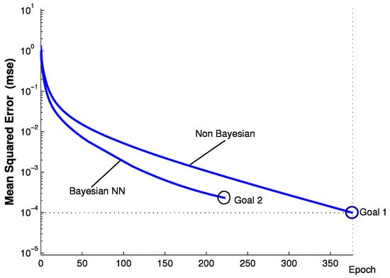
Figure 7. Non-Bayesian BP neural networks (non-Bayesian) versus BP neural networks with Bayesian regularization (Bayesian NN) in terms of training times.

Table 5. Weights after training.

Indicator	SO${}_2$	NO${}_2$	PM${}_{10}$	Dustfall	pH	AQI
Weights	0.2280	0.1023	0.1718	0.1602	0.2239	0.1125

In the next step, we take GDP per capita (perGDP) into account. Similarly, we also apply entropy method to train seven weights together and obtain the results as shown in Table 6.

Table 6. Weights after training (including GDP).

Indicator	SO${}_2$	NO${}_2$	PM${}_{10}$	Dustfall	pH	AQI	PerGDP
Weights	0.1619	0.0797	0.1107	0.1017	0.1470	0.0734	0.3257

Since the weight of perGDP is too large and has to be adjusted, we then apply the improved entropy method (according to Algorithm 1) to recalculate the weight and obtain the corrected weights in Table 7.

Table 7. Weights by improved entropy (including GDP).

Indicator	SO${}_2$	NO${}_2$	PM${}_{10}$	Dustfall	pH	AQI	PerGDP
Weights	0.0472	0.0126	0.0126	0.0126	0.0126	0.0126	0.25

Similarly, we use BP neural network to train the weights again and obtain the final results as shown in Table 8.

Table 8. Weights after training (including GDP).

Indicator	SO${}_2$	NO${}_2$	PM${}_{10}$	Dustfall	pH	AQI	PerGDP
Weights	0.0557	0.0272	0.0093	0.0069	0.0230	0.0064	0.2353

3.3. TOPSIS Evaluation

We then use TOPSIS to evaluate all of the indicators of air pollution. In particular, we first construct weighted decision matrix $V={(v_{ij})}_{m\times n}$ after determining the weights in the previous procedure. Table 9 lists the results.

Table 9. Normalization for TOPSIS in air pollution.

Year	SO${}_2$	NO${}_2$	PM${}_{10}$	Dustfall	pH	AQI
1996	0.00790	0.00258	0.00476	0.00002	0.02246	0.00663
1997	0.00790	0.00143	0.00134	0.00037	0.02181	0.00587
1998	0.00691	0.00001	0.00007	0.00157	0.02135	0.00485
1999	0.01184	0.00086	0.00002	0.00402	0.01555	0.00357
2000	0.01382	0.00646	0.00364	0.00699	0.01322	0.00791
2001	0.01184	0.00660	0.00922	0.00805	0.01903	0.00459
2002	0.01086	0.00631	0.00952	0.00655	0.00510	0.00255
2003	0.00888	0.00646	0.01041	0.00752	0.00005	0.00434
2004	0.00691	0.00631	0.00959	0.01014	0.00348	0.00383
2005	0.00592	0.00703	0.01101	0.01043	0.00603	0.00587
2006	0.00493	0.00716	0.01116	0.00849	0.00371	0.00587
2007	0.00099	0.00660	0.01123	0.00873	0.00278	0.00536
2008	0.00007	0.00574	0.01086	0.00905	0.00441	0.00689
2009	0.00691	0.00574	0.01145	0.01057	0.00534	0.00791
2010	0.00987	0.00531	0.01123	0.01000	0.01067	0.00765
2011	0.01184	0.00545	0.01183	0.01042	0.01717	0.00969
2012	0.02073	0.00574	0.01202	0.01172	0.01090	0.01044
2013	0.01777	0.00488	0.01004	0.01135	0.01067	0.00002
2014	0.02961	0.00560	0.01086	0.01182	0.01090	0.00332
2015	0.03251	0.00603	0.01153	0.01240	0.01926	0.00536

We next calculate the relative distance from the sample point to the optimal sampling point according to Equation (12) and obtain the results as shown in Table 10. In addition, Table 10 also lists the rankings of $C(\mathrm{air}\mathrm{pollution})$ ordered by years. In particular, it is shown in Table 10 that $C(\mathrm{air}\mathrm{pollution})$ in year 2014 is the most serious, while the air quality in year 2010 is the best. This result is contradictory to our common sense that the air quality is becoming worse, especially in China.

Table 10. $D_i^{+}$, $D_i^{-}$, $C(\mathrm{Air}\mathrm{Pollution})$.

$\mathit{Address}$	${\mathit{D}}_{\mathit{i}}^{\mathbf{+}}$	${\mathit{D}}_{\mathit{i}}^{\mathbf{-}}$	$\mathit{C}(\mathbf{Air}\mathbf{Pollution})$	Ranking
1996	0.0187	0.0235	0.5565	13
1997	0.0199	0.0239	0.5460	15
1998	0.0199	0.0230	0.5365	16
1999	0.0216	0.0203	0.4848	18
2000	0.0155	0.0221	0.5879	11
2001	0.0160	0.0264	0.6219	8
2002	0.0120	0.0178	0.5982	10
2003	0.0126	0.0174	0.5805	12
2004	0.0092	0.0172	0.6511	6
2005	0.0072	0.0187	0.7230	4
2006	0.0095	0.0170	0.6418	7
2007	0.0106	0.0165	0.6098	9
2008	0.0078	0.0173	0.6894	5
2009	0.0072	0.0189	0.7240	3
2010	0.0060	0.0217	0.7848	1
2011	0.0099	0.0270	0.7313	2
2012	0.0242	0.0298	0.5518	14
2013	0.0251	0.0261	0.5096	17
2014	0.0478	0.0358	0.4284	20
2015	0.0496	0.0418	0.4577	19

Similarly, we then use TOPSIS to evaluate all of the indicators including GDP (per capita) and air pollution indicators. Table 11 presents the results. We next calculate the relative proximity from sample point to the optimal sampling point according to Equation (12). Table 12 lists the positive and negative distance values.

Table 11. Normalization for TOPSIS in air pollution and GDP.

Year	SO${}_2$	NO${}_2$	PM${}_{10}$	Dustfall	pH	AQI	$\mathit{GDP}$
1996	0.00193	0.00069	0.00026	0.00000	0.00231	0.00038	0.00007
1997	0.00193	0.00038	0.00007	0.00002	0.00224	0.00033	0.00065
1998	0.00169	0.00000	0.00000	0.00007	0.00219	0.00028	0.00107
1999	0.00289	0.00023	0.00000	0.00017	0.00160	0.00020	0.00144
2000	0.00338	0.00172	0.00020	0.00030	0.00136	0.00045	0.00157
2001	0.00289	0.00175	0.00050	0.00035	0.00195	0.00026	0.00212
2002	0.00265	0.00168	0.00052	0.00028	0.00052	0.00015	0.00268
2003	0.00217	0.00172	0.00056	0.00032	0.00000	0.00025	0.00329
2004	0.00169	0.00168	0.00052	0.00044	0.00036	0.00022	0.00465
2005	0.00145	0.00187	0.00060	0.00045	0.00062	0.00033	0.00595
2006	0.00121	0.00190	0.00060	0.00037	0.00038	0.00033	0.00762
2007	0.00024	0.00175	0.00061	0.00038	0.00029	0.00030	0.00970
2008	0.00002	0.00153	0.00059	0.00039	0.00045	0.00039	0.01340
2009	0.00169	0.00153	0.00062	0.00046	0.00055	0.00045	0.01535
2010	0.00241	0.00141	0.00061	0.00043	0.00110	0.00044	0.01834
2011	0.00289	0.00145	0.00064	0.00045	0.00176	0.00055	0.02191
2012	0.00506	0.00153	0.00065	0.00050	0.00112	0.00059	0.02618
2013	0.00434	0.00130	0.00054	0.00049	0.00110	0.00000	0.02982
2014	0.00723	0.00149	0.00059	0.00051	0.00112	0.00019	0.03326
2015	0.00794	0.00160	0.00062	0.00053	0.00198	0.00030	0.03623

Table 12. $D_i^{+}$, $D_i^{-}$, C in air pollution and GDP.

Year	${\mathit{D}}_{\mathit{i}}^{\mathbf{+}}$	${\mathit{D}}_{\mathit{i}}^{\mathbf{-}}$	$\mathit{C}(\mathbf{Air}\mathbf{Pollution}\mathbf{and}\mathbf{GDP})$	Ranking
1996	0.0041	0.0023	0.3634	20
1997	0.0040	0.0031	0.4366	17
1998	0.0036	0.0030	0.4501	16
1999	0.0058	0.0036	0.3837	19
2000	0.0062	0.0043	0.4098	18
2001	0.0047	0.0044	0.4832	14
2002	0.0047	0.0041	0.4674	15
2003	0.0038	0.0043	0.5324	13
2004	0.0026	0.0051	0.6606	12
2005	0.0027	0.0062	0.6922	11
2006	0.0030	0.0077	0.7209	8
2007	0.0027	0.0097	0.7793	6
2008	0.0021	0.0135	0.8628	2
2009	0.0023	0.0151	0.8655	1
2010	0.0037	0.0182	0.8303	3
2011	0.0045	0.0218	0.8301	4
2012	0.0094	0.0263	0.7364	7
2013	0.0082	0.0302	0.7856	5
2014	0.0145	0.0339	0.7009	10
2015	0.0156	0.0369	0.7032	9

As shown in Table 12, the year 1996 has the lowest value of $C(\mathrm{air}\mathrm{pollution}\mathrm{and}\mathrm{GDP})$, implying that there was serious air pollution in 1996 while the economic development was also behind. In addition, Table 12 also indicates that the year 2009 has the highest value of $C(\mathrm{air}\mathrm{pollution}\mathrm{and}\mathrm{GDP})$, implying that there was a significant increment in GDP in the year 2009 while the air pollution was maintained low. This result indicates that the high-speed economic development can be obtained with the low air pollution at the same time if we can take effective countermeasures.

To further illustrate the relation between air pollution and GDP, we present the TOPSIS evaluation scores of $C(\mathrm{air}\mathrm{pollution})$ and $C(\mathrm{air}\mathrm{pollution}\mathrm{and}\mathrm{GDP})$, respectively, as shown in Figure 8 according to time series (from 1996 to 2015). As shown in Figure 8, the evaluation scores of GDP have been rising steadily with time, implying the high-speed economic development. Moreover, Figure 8 also shows that the evaluation scores of air pollution have fluctuated from time to time. In other words, the evaluation scores of air pollution have grown in some years while having dropped in some years. It is contradictory to our common sense that the air quality always becomes worse. More specifically, it is shown in Figure 8 that the evaluation scores of air pollution have first grown and have reached the peak in the year 2010 while having dropped down after 2010. This may be owed to the new environment protection measures that the Chinese government has taken recently.

Figure 8. Air pollution and GDP time series.

4. Conclusions and Future Works

Air pollution has a significant impact on the sustainable development of cities, especially for cities in developing countries. How to effectively evaluate the impacts of air pollution on socioeconomic development is an important issue in the sustainability of city development. However, it is quite difficult to conduct an effective evaluation on the impact of air pollution since the conventional evaluation is mainly based on the experience or the domain knowledge of environment experts, which inevitably have bias or subjectivity, consequently leading to a deviation or inaccuracy in air pollution evaluation.

In this paper, we propose a novel Multiple Criteria Decision Making (MCDM) framework to address the above concerns. In particular, our proposed MCDM method is based on an improved TOPSIS, in which Bayesian regularization and BP neural networks have been used to train the weights of multiple indicators. We apply our framework to evaluate the air pollution and the economic development of Wuhan city, which is a typical developing city in China. Our empirical results show that the evaluation scores of air pollution have fluctuated from time to time; this effect is contradictory to the common sense that air pollution always becomes worse. In fact, our results imply that sustainable socioeconomic development can be achieved without environment deterioration if we can take effective environment protection measures. We believe that the appropriate pollution control technologies, the enforcement of emissions reduction policy and the adjustment of industry layout will reduce the air pollution and support the sustainable urban development. One of our future studies is to conduct a fine-grained study on the impacts of various environment protection measures on air pollution and socioeconomic development, which is also an MCDM problem and is expected to be solved in a different approach.

References

- Pope, C.A.; Burnett, R.T.; Thun, M.J.; Calle, E.E.; Krewski, D.; Ito, K.; Thurston, G.D. Lung Cancer Cardiopulmonary Mortality, and Long-term Exposure to Fine Particulate Air Pollution. JAMA 2002, 287, 1132–1141. [Google Scholar] [CrossRef] [PubMed]
- Pope, C.A.; Jerrett, M.; Burnett, R.T. Long-Term Ozone Exposure and Mortality. N. Engl. J. Med. 2009, 360, 1085–1095. [Google Scholar]
- Lepeule, J.; Bind, M.A.C.; Baccarelli, A.A. Epigenetic Influences on Associations between Air Pollutants and Lung Function in Elderly Men. N. Engl. J. Med. 2014, 122, 1085–1095. [Google Scholar]
- Tanaka, S. Environmental regulations on air pollution in China and their impact on infant mortality. J. Health Econ. 2015, 42, 90–103. [Google Scholar] [CrossRef] [PubMed]
- Rao, S.; Klimont, Z.; Smith, S.J.; Dingenen, R.V.; Dentener, F.; Bouwman, L.; Riahi, K.; Amann, M.; Bodirsky, B.L.; van Vuuren, D.P.; et al. Future air pollution in the Shared Socio-economic Pathways. Glob. Environ. Chang. 2017, 42, 346–358. [Google Scholar] [CrossRef]
- Li, P. 1.1 Trillion Yuan in Economic Losses from Pollution in 2010, China Report Says. Available online: http://www.scmp.com/news/china/article/1201364/11-tr-yuan-economic-losses-pollution-2010-china-report-says (accessed on 29 May 2017).
- Cheng, H.; Small, M.J.; Pekney, N.J. Application of nonparametric regression and statistical testing to identify the impact of oil and natural gas develop mentonlocal air quality. Atmos. Environ. 2015, 119, 381–392. [Google Scholar] [CrossRef]
- Nduwayezu, J.B.; Ishimwe, T.; Niyibizi, A. Quantification of Air Pollution in Kigali City and Its Environmental and Socio-Economic Impact in Rwanda. Am. J. Environ. Eng. 2015, 5, 106–119. [Google Scholar]
- Alvarado, M.; Gonzalez, F.; Erskine, P.; Cliff, D.; Heuff, D. A Methodology to Monitor Airborne PM10 Dust Particles Using a Small Unmanned Aerial Vehicle. Sensors 2017, 17, 343. [Google Scholar] [CrossRef] [PubMed]
- Cho, H.S.; Choi, M.J. Effects of Compact Urban Development on Air Pollution: Empirical Evidence from Korea. Sustainability 2014, 6, 5968–5982. [Google Scholar] [CrossRef]
- Liu, H.L.; Shen, Y.S. The Impact of Green Space Changes on Air Pollution and Microclimates: A Case Study of the Taipei Metropolitan Area. Sustainability 2014, 6, 8827–8855. [Google Scholar] [CrossRef]
- Vallero, D.A. Air Pollution Monitoring Changes to Accompany the Transition from a Control to a Systems Focus. Sustainability 2016, 8, 1216. [Google Scholar] [CrossRef]
- Zhao, J.; Chen, S.; Wang, H. Quantifying the impacts of socio-economic factors on air quality in Chinese cities from 2000 to 2009. Environ. Pollut. 2012, 167, 148–154. [Google Scholar] [CrossRef] [PubMed]
- Yang, C.; Yang, H.; Guo, S.; Wang, Z.; Xu, X.; Duan, X.; Kan, H. Alternative ozone metrics and daily mortality in Suzhou: The China Air Pollution and Health Effects Study (CAPES). Sci. Total Environ. 2012, 426, 83–89. [Google Scholar] [CrossRef] [PubMed]
- Tang, D.; Li, T.Y.; Chow, J.C. Air pollution effects on feral and child development: A cohort comparison in China. Environ. Pollut. 2014, 185, 90–96. [Google Scholar] [CrossRef] [PubMed]
- Almanza, V.; Batyrshin, I.; Sosa, G. Multi-criteria selection of an Air Quality Model configuration based on quantitative and linguistic evaluations. Expert Syst. Appl. 2014, 41, 869–876. [Google Scholar] [CrossRef]
- Preisler, H.K.; Schweizer, D.; Cisneros, R.; Procter, T.; Ruminski, M.; Tarnay, L. A statistical model for determining impact of wildland fires on Particulate Matter (PM2.5) in Central California aided by satellite imagery of smoke. Environ. Pollut. 2015, 205, 340–349. [Google Scholar] [CrossRef] [PubMed]
- Jaramilloa, P.; Mullerb, N.Z. Air pollution emissions and damages from energy production in the U.S.: 2002–2011. Energy Policy 2016, 3, 202–211. [Google Scholar] [CrossRef]
- Donga, L.; Liang, H. Spatial analysis on China’s regional air pollutants and CO2 emissions: Emission pattern and regional disparity. Atmos. Environ. 2014, 92, 280–291. [Google Scholar] [CrossRef]
- Yoon, K.P.; Hwang, C.L. Multiple Attribute Decision Making: An Introduction; Sage Publications: Thousand Oaks, CA, USA, 1995; Volume 104. [Google Scholar]
- Chen, J.K.; Chen, I.S. Using a novel conjunctive MCDM approach based on DEMATEL, fuzzy ANP, and TOPSIS as an innovation support system for Taiwanese higher education. Expert Syst. Appl. 2010, 37, 1981–1990. [Google Scholar] [CrossRef]
- Kahraman, C. Fuzzy Multi-Criteria Decision Making: Theory and Applications with Recent Developments; Springer: New York, NY, USA, 2008; Volume 16. [Google Scholar]
- Ferreira, L.; Borenstein, D. A fuzzy-Bayesian model for supplier selection. Expert Syst. Appl. 2012, 39, 7834–7844. [Google Scholar] [CrossRef]
- Sipahi, S.; Timor, M. The analytic hierarchy process and analytic network process: An overview of applications. Manag. Decis. 2010, 48, 775–808. [Google Scholar] [CrossRef]
- Velasquez, M.; Hester, P.T. An analysis of multi-criteria decision making methods. Int. J. Op. Res. 2013, 10, 56–66. [Google Scholar]
- Behzadian, M.; Otaghsara, S.K.; Yazdani, M.; Ignatius, J. A state-of the-art survey of TOPSIS applications. Expert Syst. Appl. 2012, 39, 13051–13069. [Google Scholar] [CrossRef]
- Hafezalkotob, A.; Hafezalkotob, A. Extended MULTIMOORA method based on Shannon entropy weight for materials selection. J. Ind. Eng. Int. 2016, 12, 1–13. [Google Scholar] [CrossRef]
- Dymova, L.; Sevastjanov, P.; Tikhonenko, A. An approach to generalization of fuzzy TOPSIS method. Inf. Sci. 2013, 238, 149–162. [Google Scholar] [CrossRef]
- Büyüközkan, G.; Çifçi, G. A novel hybrid MCDM approach based on fuzzy DEMATEL, fuzzy ANP and fuzzy TOPSIS to evaluate green suppliers. Expert Syst. Appl. 2012, 39, 3000–3011. [Google Scholar] [CrossRef]
- Baykasoglu, A.; Kaplanoglu, V.; Durmusoglu, Z.D.; Sahin, C. Integrating fuzzy DEMATEL and fuzzy hierarchical TOPSIS methods for truck selection. Expert Syst. Appl. 2013, 40, 899–907. [Google Scholar] [CrossRef]
- Pan, S.J.; Yang, Q. A survey on transfer learning. IEEE Trans. Knowl. Data Eng. 2010, 22, 1345–1359. [Google Scholar] [CrossRef]
- Ministry of Envirmental Protection of the People’s Republic China. Ambient Air Quality Standards; Ministry of Envirmental Protection of the People’s Republic China: Beijing, China, 2012.
- Gray, R.M. Entropy and Information Theory; Springer: Berlin, Germany, 2011. [Google Scholar]
- Lotfi, F.H.; Fallahnejad, R. Imprecise Shannon’s entropy and multi attribute decision making. Entropy 2010, 12, 53–62. [Google Scholar] [CrossRef]
- Haykin, S. Neural Networks and Learning Machines, 3rd ed.; Pearson: London, UK, 2009. [Google Scholar]
- Ticknor, J.L. A Bayesian regularized artificial neural network for stock market forecasting. Expert Syst. Appl. 2013, 40, 5501–5506. [Google Scholar] [CrossRef]
- Mirjalili, S. SCA: A Sine Cosine Algorithm for solving optimization problems. Knowl. Based Syst. 2016, 96, 120–133. [Google Scholar] [CrossRef]
- Mirjalili, S.; Saremi, S.; Mirjalili, S.M.; dos S. Coelho, L. Multi-objective grey wolf optimizer: A novel algorithm for multi-criterion optimization. Expert Syst. Appl. 2016, 47, 106–119. [Google Scholar] [CrossRef]
- Mirjalili, S.; Jangir, P.; Saremi, S. Multi-objective ant lion optimizer: A multi-objective optimization algorithm for solving engineering problems. Appl. Intell. 2017, 46, 79–95. [Google Scholar] [CrossRef]
- Wuhan Environmental Protection Bureau. Air Quality of Wuhan City (1996–2015); The Communique of Ambient Air Quality of Wuhan Publised by Wuhan Environmental Protection Bureau; Wuhan Environmental Protection Bureau: Wuhan, China.
- Wuhan Municipal Bureau of Statistics. Yearbook of Wuhan Municipal Bureau of Statistics (1996–2015); Wuhan Municipal Bureau of Statistics: Wuhan, China. (In Chinese)
- Jolliffe, I. Principal Component Analysis; Wiley Online Library: Hoboken, NJ, USA, 2002. [Google Scholar]
- Abdi, H.; Williams, L.J. Principal component analysis. In Wiley Interdisciplinary Reviews: Computational Statistics; Wiley Online Library: Hoboken, NJ, USA, 2010; Volume 2, pp. 433–459. [Google Scholar]
- De Winter, J.D.; Dodou, D.; Wieringa, P. Exploratory factor analysis with small sample sizes. Multivar. Behav. Res. 2009, 44, 147–181. [Google Scholar] [CrossRef] [PubMed]
- Bandalos, D.L.; Boehm-Kaufman, M.R. Four common misconceptions in exploratory factor analysis. Statistical and Methodological Myths and Urban Legends: Doctrine, Verity and Fable in the Organizational and Social Sciences; Routledge/Taylor & Francis Group: New York, NY, USA, 2009; pp. 61–87. [Google Scholar]
- Peres-Neto, P.R.; Jackson, D.A.; Somers, K.M. How many principal components? Stopping rules for determining the number of non-trivial axes revisited. Comput. Stat. Data Anal. 2005, 49, 974–997. [Google Scholar] [CrossRef]
© 2017 by the authors. Licensee MDPI, Basel, Switzerland. This article is an open access article distributed under the terms and conditions of the Creative Commons Attribution (CC BY) license (http://creativecommons.org/licenses/by/4.0/).