On Production and Green Transportation Coordination in a Sustainable Global Supply Chain

Abstract

This paper addresses a coordination problem of production and green transportation and the effects of production and transportation coordination on supply chain sustainability in a global supply chain environment with the consideration of important realistic characteristics, including parallel machines, different order processing complexities, fixed delivery departure times, green transportation and multiple transportation modes. We formulate the measurements for carbon emissions of different transportation modes, including air, sea and land transportation. A hybrid genetic algorithm-based optimization approach is developed to handle this problem, in which a hybrid genetic algorithm and heuristic procedures are combined. The effectiveness of the proposed approach is validated by means of various problem instances. We observe that the coordination of production and green transportation has a large effect on the overall supply chain sustainability, which can reduce the total supply chain cost by 9.60% to 21.90%.

1. Introduction

With the increasing globalization, more and more managers are aware of the importance of the coordination and cooperation of supply chain operations. Coordination of production and transportation operations aims to investigate how to schedule production orders and how to deliver the finished products to customers in a joint and integrated manner, in which production and transportation operations are highly integrated to enhance the supply chain performance and therefore achieve higher supply chain sustainability [1,2].

In a global make-to-order (MTO) environment, it is common that the distribution is performed by a third-party logistics company such as UPS or DHL, which provides multiple transportation modes such as air, sea and land transportation. Fourteen percent of 2010 global greenhouse gas emissions is attributed to transportation [3]. Reducing energy consumption and carbon emission in transportation is thus critical. This paper investigates the coordination of production and transportation operations with the consideration of multiple transportation modes and carbon emissions, called the coordination problem of production and green transportation (short for CPGT problem).

The study on the coordination problem of production and transportation operations (CPTO problem) can be traced back to the 1980s [2]. Since then, many researchers have studied the CPTO problems from different perspectives. Moon et al. [4] study the CPTO problem with the objective of minimizing the maximum completion time, and establish a mixed integer linear programming model. Considering the particularity of concrete transportation, Garcia et al. [5] deal with a CPTO problem in a scenario of no-wait, immediate delivery to the customer site. Chen and Vairaktarakis [6] study two classes of CPTO problems motivated by applications in the computer and food catering service industries.

In 2010, Chen [1] made a comprehensive survey on CPTO problems. After that, Agnetis et al. [7] address a CPTO problem with semi-products belonging to the same manufacturer. These semi-products need to be processed in one production location and transported to another production location by a third-party logistics provider. Kaya et al. [8] study a CPTO problem in a deterministic inventory system with a single supplier and a single retailer, and they investigate both integrated model and a decentralized model. Hajiaghaei-Keshteli et al. [9] study a CPTO problem of synchronization of production and rail transportation. The objective of this problem is to schedule production and allocate rail transportation of orders while optimizing customer service at the minimum total cost. Lee et al. [10] construct a CPTO model in a make-to-order producer-buyer supply chain with the objective of minimizing the total cost including transportation cost. Koc et al. [11] investigate a CPTO problem for the production and delivery of a set of orders with two vehicle types for outbound shipments, and analyze the manufacturer’s planning problem under different delivery policies.

Most of previous studies on CPTO problems focused on simple realistic characteristics, such as single transportation mode [8], the same order size [7,12], the same order processing complexity [5,13] and flow production [14]. However, previous studies seldom considered such more complicated realistic features as fixed vehicle departure times, multiple transportation modes and green transportations.

These various complicated realistic features exist in practice. Most companies worldwide now rely on third-party logistics providers for their daily distribution and transportation needs. Many third-party service providers have daily fixed package pickup times. The CPTO problems thus have to consider fixed vehicle departure times. In addition, multiple transportation modes usually exist in practice, each of which corresponds to a certain combination of transportation speed and capacity. Li et al. [15] study a CPTO problem in a global supply chain with air transportation in the consumer electronics industry, in which the transportation departure time for each order is fixed by the airline. Stecke et al. [16] study a CPTO problem with a commit-to-delivery mode of business, and the vehicle from a third-party logistics company arrive at the same time, which depicts a planning horizon that starts at a fixed time. Azadian et al. [17] study a CPTO problem of a make-to-order contract manufacturer which considers multiple transportation modes. Memari et al. [18] study a CPTO problem in green supply chain, and the objectives of the problem are minimizing the total cost as well as minimizing the environmental impact of logistic network. However, CPTO problems, which consider fixed delivery departure times, multiple transportation modes and green transportation simultaneously, have not been investigated so far, although these problems are widespread in some real-world supply chains such as apparel and footwear. This paper thus investigates a CPTO problem with the consideration of these realistic features, called the CPGT problem.

Due to the consideration of these realistic features, the CPGT problem is a complex CPTO problem. It is well known that the CPTO problem with simple realistic features is a non-deterministic polynomial-hard problem [1]. With the increase of complexity and problem size of CPTO problems, it is well known that traditional techniques, including mathematical programming techniques, heuristic techniques and traditional intelligent techniques, have difficulties in handling these more complex CPTO problems. González and Vela [19] have pointed out that the running time of traditional optimization techniques in handling some complex CPTO instances with 60 or more jobs is prohibitive, taking several weeks in some extreme cases. For larger instances, the computation time may increase exponentially.

Various optimization techniques have been used to solve these CPTO problems, which involve mathematical programming, heuristics and traditional intelligent algorithms, and so forth. Lee and Fu [10] use a network optimization method to solve two kinds of CPTO problems. Garcia et al. [5] propose a heuristic algorithm to obtain the near-optimal solution to a CPTO problem. Viergutz et al. [20] use a branch and bound method to solve a single-plant CPTO problem with the objective of minimizing completion time. Some researchers use evolutionary techniques to solve CPTO problems. Moon et al. [4] develop a new evolutionary search approach based on a topological sort to solve a CPTO problem with multiple manufacturing sites. Ullrich [21] introduce a genetic algorithm-based approach to solve a CPTO problem consisting of two sub-problems. The first addresses the scheduling of a set of jobs on parallel machines with machine-dependent ready times while the second focusses on making the delivery decisions of completed jobs.

Hybrid genetic algorithms, which are also referred to as genetic local search algorithms, can obtain good performance with faster computation time and have excellent performance in solving various complex optimization problems [22]. Hybrid genetic algorithms have also been used to solve complex CPTO problems effectively [23,24]. This paper thus proposes a hybrid genetic algorithm-based optimization (HGAO) approach to solve the CPGT problem investigated.

The structure of this paper is as follows. Section 2 presents the problem investigated and elaborates how to measure the carbon emissions in different transportation modes. Section 3 describes the proposed HGAO approach. In Section 4, the numerical experiments are presented and experimental results are analyzed to demonstrate the effectiveness of the HGAO approach. Section 5 discusses the performance of the proposed approach and the effects of coordinated production and green transportation. Finally, Section 6 summarizes this paper and provides the future research directions.

2. Problem Statement

2.1. Problem Description

At the beginning of a scheduling horizon, the plant receives a set of orders from customers all around the world and commits a delivery date for each order. The plant needs to process these orders on a dedicated machine of this plant and delivers the finished products to customers by a third-party logistics company. Each order contains a set of jobs. Different orders could have different order sizes and the complexities of different jobs could be different. The plant could produce multiple orders at the same time. If so, the production capacity for each order in parallel is the same. The jobs within an order must be processed continuously in turn. To respond quickly to customer orders, the plant integrates the machine scheduling and distribution operations together, which first needs to determine the production beginning time of each order in the plant. After the production of an order is completed, finished products need to be delivered to customer destinations. In each order, the products with the same destination are defined as a product batch, which may consist of products from different jobs. Some product batches may arrive the customer destination in advance or late, which lead to earliness or tardiness penalty, respectively. Third-party logistics companies are responsible for transporting finished products to customer-specified destinations, which provide multiple transportation modes including sea, land and air transportation. Different transportation modes correspond to different unit transportation costs, time and carbon emissions. The plant needs to select a suitable transportation mode dynamically to achieve the supply chain objective.

Without the loss of generality, the investigated problem assumes that: (1) the start time of scheduling horizon is zero; (2) there is no shortage of raw materials; and (3) the third-party logistics company has enough vehicles to complete given transportation tasks.

The investigated CPGT problem needs to determine the values of three decision variables, $S_{ik}$ and $M_{ikm}$. $R_{i{i}^{\prime }}$ is 1 if order $i^{\prime }$ is the immediate succeeding of order $i$, otherwise it is 0. $S_{ik}$ denotes the departure time of product batch $(i,k)$. $M_{ikm}$ is 1 if the product batch $(i,k)$ is transported via transportation mode $m$ otherwise it is 0. The objective is to minimize the total supply chain cost, including holding cost, transportation cost, earliness and tardiness cost, and carbon emission cost. We do not consider the production cost because the production cost of each order in the plant is a constant. The objective can be formulated as follows:

$$\min F\left(R_{i{i}^{\prime }},S_{ik},M_{ikm}\right)={\displaystyle \sum _{i=1}^I{\displaystyle \sum _{k=1}^K(H{C}_{ik}+T{C}_{ik}+E{P}_{ik}+T{P}_{ik}+E{C}_{ik})}}$$

(1)

where $H{C}_{ik}$, $T{C}_{ik}$, $E{P}_{ik}$, $T{P}_{ik}$ and $E{C}_{ik}$ denote the holding cost, the transportation cost, the earliness penalty, the tardiness penalty and the carbon emission cost of product batch $(i,k)$ respectively.

2.2. Measurement for Transportation Carbon Emissions

With different transportation modes, fuel consumptions are apparently different to transport products from one place to another. This section presents how to calculate the carbon emissions under different transportation modes in detail.

2.2.1. Carbon Emission of Sea Transportation

For sea transportation, carbon emissions are mainly from shipping fuel consumption. The amount of fuel consumed by shipping depends on its load factor, frequency of sailing, speed, distance involved, and fuel efficiency [25]:

$$C^{fu}=\frac{d}{v}\times F^{fu}\times \frac{W}{SL}$$

(2)

where $C^{fu}$ denotes the consumption of fuel type $fu$ (e.g., heavy oil and diesel), $d$ the distance from the plant to the destination (km), $v$ the transport speed (27.78 km/h), $F^{fu}$ the main engine fuel economy of fuel type $fu$, $W$ the number of containers (unit: Twenty-foot Equivalent Unit (TEU)), and $SL$ the containership capacity (444 TEU/trip). The amount of CO₂ emissions is estimated by multiplying the fuel consumption for heavy oil and diesel and the emission factor.

$$E_s=C^{fu}\times \zeta$$

(3)

where $E_s$ denotes the CO₂ emission (ton) for shipping, and $\zeta$ is the emission factor of CO₂ for containerships of heavy oil and diesel, which is in line with maritime fuels generally, namely, 3.11 ton of CO₂ per heavy oil ton and 3.1 ton of CO₂ per diesel ton.

For simplicity, assuming that the shipping speed remains unchanged. Let $W=\frac{Q}{Q_{TEU}}$, where $Q$ is the number of product batch pieces, $Q_{TEU}$ is the container capacity (500 pieces/TEU), and there is only one type of fuel consumed, engines with diesel $F^{fu}$ consuming 0.04 ton/h and emission factor $\zeta$ is 3.1 ton. Set $\varphi =\frac{F^{fu}\cdot \zeta }{v\cdot SL\cdot Q_{TEU}}$, and it is clear that $\varphi$ is constant, which equals 2.01 × 10⁻⁸. E_s (ton CO₂) can thus be expressed as

$$E_s=\varphi \cdot d\cdot Q=2.01\times {10}^{-8}\cdot d\cdot Q$$

(4)

2.2.2. Carbon Emission of Land Transportation

For land transportation, according to the definition of energy consumption given by Bektas and Laporte [26], we have

$$E_v=\gamma \cdot d\cdot \theta \cdot [\alpha \times (w+f)+\beta v^2]$$

(5)

where $E_v$ is the carbon emission of vehicle, $\gamma$ is the fuel emission factor, $\theta$ is the conversion factor that is defined as liter of fuel consumed per joule of energy, $\alpha$ is the road-specific constant, $w$ is the actual load of vehicle, $f$ is the curb weight of one vehicle, $d$ is the distance of transportation, $\beta$ is vehicle-specific constant, $v$ is the speed of vehicle.

For simplicity, set $w=\rho \cdot Q$, where $\rho$ is the weight of the product (per piece). According to formula [5], we have

$$E_v=(\gamma \cdot \alpha \cdot (\rho \cdot Q+f)+\gamma \cdot \beta \cdot v^2)\cdot \theta \cdot d$$

(6)

According to the data from the U.S. Energy Information Administration, 2.681 kg CO₂ will be emitted if 1 L diesel is consumed [27]. And set $r_1=\gamma \cdot \alpha$ and $r_2=\gamma \cdot \beta \cdot v^2$. It is clear that $r_1$ and $r_2$ are constants. Then $E_v$ can be expressed as

$$E_v=(r_1\cdot (\rho \cdot Q+f)+r_2)\cdot \theta \cdot d$$

(7)

2.2.3. Carbon Emission of Air Transportation

For air transportation, carbon emissions are generated in two main parts: landing/take-off cycle (LTO) and cruise of aircrafts. The analysis about these two parts has been given by Chao [28]. The related greenhouse gas is only CO₂. For simplicity, assuming that the type of aircraft and fuel is the same, and the transportation consumption is proportional to the distance. $E_a$ can thus be expressed as:

$$E_a=cf\times \rho \cdot d\cdot Q$$

(8)

where $cf$ is the carbon footprint (kg/ton·km-CO₂ ) of the aircraft, $\rho$ is the weight (kg/piece) of the product, $Q$ is the quantity of product batch, and $d$ is the distance (km) between destination and plant. This paper calculates the carbon footprint of aircraft by using the medium-sized freighter A330-200F (68 tons) for air transportation. Then we have

$$cf=\{\begin{array}{cc}0.752& d<1000\\ 0.461& 1000\le d<3000\\ 0.410& 3000<d\end{array}$$

(9)

On the basis of the measurement for carbon emissions of different transportation modes, the carbon emission $C{E}_{ik}$ of product batch $(i,k)$ via a transportation mode is formulated as follows.

$$C{E}_{ik}=\lambda \cdot [M_{ik1}\times \varphi d_{ik}\times Q_{ik}+M_{ik2}\times (r_1\cdot (\rho Q_{ik}+f)+r_2)\cdot \theta \cdot d_{ik}+M_{ik3}\times cf\times \rho d_{ik}{Q}_{ik}]$$

(10)

3. Methodology

The hybrid genetic algorithm-based optimization (HGAO) approach combines hybrid genetic algorithm with some heuristic procedures, which aims to generate the best solutions to the investigated CPGT problem.

3.1. Overview of Hybrid Genetic Algorithm-Based Optimization Approach

The investigated CPGT problem needs to determine the values of three decision variables, $R_{i{i}^{\prime }}$, $S_{ik}$ and $M_{ikm}$. These values are interdependent. For instance, $S_{ik}$ depends on the production completion date of product batch $(i,k)$, which is determined by the production sequence $R_{i{i}^{\prime }}$ of orders. To effectively solve this problem, an HGAO approach is developed by integrating a hybrid genetic optimization process and some heuristic procedures. The hybrid genetic optimization process is used to find the best order sequence solutions {$R_{i{i}^{\prime }}$} to the investigated CPGT problem. The heuristic procedures are proposed to calculate the supply chain cost (including carbon emission cost) and values of other variables based on the candidate production sequence solution. Figure 1 shows the flow chart of the HGAO approach. The steps involved are described as follows in detail.

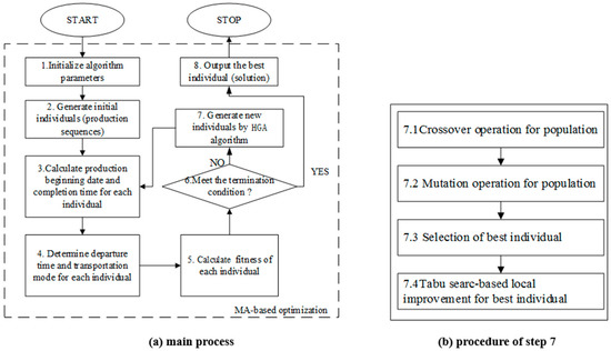
Figure 1. Flow chart of the hybrid genetic algorithm-based optimization (HGAO) approach.

The main process of the HGAO approach is shown in Figure 1a. First, the values of algorithm parameters are initialized, including population size, mutation rate, crossover rate, tabu size, and so on. In step 2, we randomly generate the population of initial individuals, each of which indicates the production precedence of orders in the plant. Next, steps 3–7 constitute the iterative process for hybrid genetic optimization, which iteratively find the best values of three decision variables. Each iteration represents a generation of the evolutionary process of HGAO approach. In steps 3–5, the values of decision variables $R_{i{i}^{\prime }}$, $S_{ik}$ and $M_{ikm}$ and the corresponding objective value are calculated based on the solution individual, the detail of which will be described in Section 3.3. If the termination condition is satisfied in step 6, the optimization process is terminated and the best solution obtained is returned as the best integrated optimization solution in step 8. Otherwise, the process returns to step 7 for generating the population of next generation. As shown in Figure 1b, step 7 consists of four sub-steps. Step 7.1–7.2 indicates that a new population is generated based on a crossover operation and a mutation operation. Step 7.3 states that the best individual of the population is selected out and preserved. Step 7.4 states that a tabu search-based local improvement is performed based on the best individual. The key operations involved will be described in detail in Section 3.2.

3.2. Key Operations in Hybrid Genetic Algorithm

The hybrid genetic algorithm is a combination of genetic algorithm and a local search process [22]. In general, the key operations in hybrid genetic algorithm include: (1) the encoding operation shows how each individual (solution) is represented; (2) the population initialization operation shows how the initial population is created; (3) the genetic operations (e.g., crossover and mutation operations) show how the offspring are generated during reproduction; and (4) a tabu search-based local improvement process. The detail of these operations are described as follows.

3.2.1. Encoding

Let $N$ denote the population size. Let $x_n$ denote the $n$th ($n\in [1,N]$) individual in the population, which represents a production sequence solution of orders in the plant. Set $x_n=(S^n,F(S^n))$, where $S^n$ denotes the candidate production sequence solution and $F(S^n)$ denotes the fitness of $S^n$. Set $S^n=(a_1^n,a_2^n,\dots ,a_I^n)$ and the value of $a_i^n$ denotes the order number of the $i$th order to be produced. For example, $x_n$ = ((3, 2, 1, 4, 5), 0.001) states that orders 3, 2, 1, 4 and 5 are produced in turn and the corresponding fitness is 0.001.

3.2.2. Population Initialization and Selection

In hybrid genetic algorithm, a set of individuals forms a population. The initial population is generated randomly for the first generation. The individuals in the population are evaluated using a fitness value. The value of fitness function is calculated according to the procedure described in Section 3.3.

The selection operator used is the tournament selection. This operator takes randomly a specified number of individuals in the population, the best individual in the selected individuals is selected as a parent and the process is repeated to complete the parental population. In this study, the offspring population is primarily composed of the following: best individuals obtained by genetic operator, new individual generated by tabu search-based local improvement and the best individual reserved from previous generations.

3.2.3. Genetic Operators

The genetic operators enhance the performance of solutions by propagating similarities and unexpected genetic characteristics to offspring. In general, the performance of evolution techniques strongly depends on the design of crossover operators while mutation tremendously influences the diversity of population [29]. This research utilizes the uniform crossover operator [30] and the inversion mutation operator [31] to generate the individuals in the offspring population.

The uniform crossover operator generates two children starting from two parents. First, the uniform crossover operator generates a binary random-index based on uniform distribution, the length of which is the same as the number of orders. And if the $i$th binary number of random-index equals 1, the $i$th gene of individual will be marked. Finally the uniform crossover completes the two children by swapping the marked genes from two parents.

The inversion mutation operator selects an operation from a single parent individual and inverts one part of the individual. The inversion mutation operator is applied to improve the solution quality.

3.2.4. Tabu Search-Based Local Improvement

Tabu search (TS) is proposed by Glover [32], which is an optimization algorithm though a simulation of human intelligence process [33]. Its search performance is completely dependent on the domain structure and initial solution, especially in the local minimum and it cannot guarantee the global optimization. By introducing a flexible storage structure and a corresponding tabu criterion, the TS can effectively find the local optimum within a small computation time.

Figure 2 gives the pseudocode of the tabu search-based local improvement process, which is described as follows. First, the tabu search is initialized by setting the tabu list to null and setting the initial current solution $x_o$ (line 1). Lines 2–13 are iterative process of tabu search. Line 3 generates neighboring solutions $\left\{x_1,x_2,\dots ,x_n\right\}$ (lines 2–3). Then, each neighboring solution is iterated (lines 4–12). In detail, line 5 checks whether the value of corresponding taboo list for candidate solution $x_i$ is 0. If so, go to line 6; otherwise go to line 12. Line 6 checks whether the candidate solution $x_i$ meets the aspiration criterion. If so, replace the best solution $x_b$ by $x_i$, setting $x_o$ = $x_i$ and update the tabu list (line 7); otherwise checks whether the candidate solution $x_i$ is the optimal value in the candidate solutions $\left\{x_1,x_2,\dots ,x_i\right\}$ (line 8). If so, replace the current solution $x_o$ by the candidate solution $x_i$ and update tabu list (line 9). The iterations of tabu search are repeated until a termination condition is met (line 13). Finally, the best solution $x_b$ is returned in line 14.

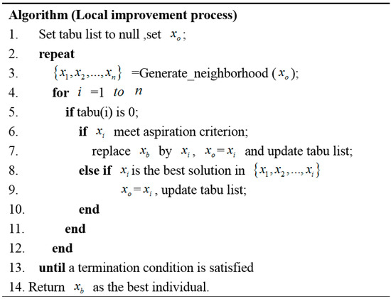
Figure 2. Pseudocode of tabu search-based local improvement process.

3.3. Calculation of Values of $S_{ik}$, $M_{ikm}$ and Fitness Function

The individual in the evolutionary process of the HGAO approach determines the production sequence $R_{i{i}^{\prime }}$ of orders, the completion date $C_i$ can then be determined. This section introduces how to decide the values of departure time $S_{ik}$ and transportation mode $M_{ikm}$, finally getting the value of fitness function of this individual based on the given production sequence of the individual.

According to the values of expected delivery date $d_i$ and production completion date $C_i$, the values of variables $S_{ik}$ and $M_{ikm}$ can be determined optimally by the following 3 rules, which can be easily proved by contradiction.

Rule 1: If no transportation mode can transport products to the destination by the expected delivery date $d_i$, then $M_{ikm}$ is set as the transportation mode with the shortest transportation time, $S_{ik}$ is equal to the production completion date $C_i$ of order $i$.

Rule 2: If multiple transportation modes can complete the transportation task by the expected delivery date $d_i$, then $M_{ikm}$ is set as the transportation mode with the longest transportation time. That is, the transportation mode with the minimal transportation cost is selected. $S_{ik}$ is determined by Rule 3.

Rule 3: If the holding cost of product batch (I, k) is greater than the earliness penalty, set $S_{ik}=\lceil C_i\rceil$; otherwise, set $S_{ik}=d_i-\lceil C_i\rceil -T{T}_{ikm}$. $T{T}_{ikm}$ denotes the transportation time of transportation mode $m$ for product batch (I, k).

After the values of these variables are determined, the value of the objective function (the total cost of the supply chain) can be calculated. The value of its fitness function can then be set as the reciprocal of the objective value.

4. Numerical Experiments

This section presents the numerical experiments to validate the performance of our approach. First, experimental data and algorithm parameters are presented in Section 4.1. The proposed HGAO approach is evaluated by three numerical experiments in Section 4.2.

4.1. Experimental Data and Algorithm Parameters

A series of numerical experiments have been conducted to evaluate the effectiveness of the proposed HGAO approach. This section presents three representative experiments in practice. Experimental data were collected from a global MTO manufacturing enterprise in China. The three experiments handle three different integrated production and transportation tasks. Similar tasks are widespread in the global labor-intensive enterprises. In each experiment case, different production tasks are processed:

(1)

Experiment 1: eight orders with 38 product batches;

(1)

Experiment 2: 10 orders with 43 product batches;

(1)

Experiment 3: 11 orders with 40 product batches.

Table 1, Table 2 and Table 3 show the information related to each order in these experiments. The values in columns 1–3 show customer number, order number and delivery destination number, respectively. Columns 4–7 show the product quantity (pieces), expected delivery date, daily earliness penalty and daily tardiness penalty ($/day) of each product batch, respectively. Column 8 shows the processing efficiency of the order. “1” “2” “3” represents the high, medium and low machining efficiency, respectively.

Table 1. Data of orders in experiment 1.

Customers	Orders	Destinations	Quantity Delivered (Piece)	Expected Delivery Date	Daily Earliness Penalty ($/Day)	Daily Tardiness Penalty ($/Day)	Complexity
C1	1	1	7500	37	1125	6000	1
	1	3	7500	37	1125	6000	1
	1	4	5000	37	750	4000	1
	1	5	5000	37	750	4000	1
	1	6	5000	37	750	4000	1
C2	2	1	7000	41	700	4900	2
	2	3	6000	41	600	4200	2
	2	4	6000	41	600	4200	2
	2	6	5000	41	500	3500	2
C3	3	1	9000	49	1350	6300	1
	3	3	9000	49	1350	6300	1
	3	4	8000	49	1200	5600	1
	3	8	8000	49	1200	5600	1
	3	9	7000	49	1050	4900	1
	3	10	7000	49	1050	4900	1
C4	4	1	12,000	54	1800	9600	1
	4	3	10,000	54	1500	8000	1
	4	4	9000	54	1350	7200	1
	4	5	9000	54	1350	7200	1
C5	5	1	6000	58	600	4800	2
	5	3	6000	58	600	4800	2
	5	6	6000	58	600	4800	2
C6	6	1	7000	62	700	4550	3
	6	3	6000	62	600	3900	3
	6	4	6000	62	600	3900	3
	6	5	6000	62	600	3900	3
	6	8	5500	62	550	3575	3
	6	9	5500	62	550	3575	3
C7	7	1	12,000	64	1800	9600	3
	7	2	9000	64	1350	7200	3
	7	9	8000	64	1200	6400	3
	7	10	8000	64	1200	6400	3
	7	13	8000	64	1200	6400	3
C8	8	9	1400	66	210	1120	2
	8	10	1400	66	210	1120	2
	8	11	1400	66	210	1120	2
	8	12	1400	66	210	1120	2
	8	13	1400	66	210	1120	2

Table 2. Data of orders in experiment 2.

Customers	Orders	Destinations	Quantity Delivered (Piece)	Expected Delivery Date	Daily Earliness Penalty ($/Day)	Daily Tardiness Penalty ($/Day)	Complexity
C1	1	1	9000	33	1350	7200	1
	1	3	7000	33	1050	5600	1
	1	4	7000	33	1050	5600	1
	1	5	6000	33	900	4800	1
	1	13	6000	33	900	4800	1
C2	2	1	5000	38	750	4000	1
	2	2	4500	38	675	3600	1
	2	3	4000	38	600	3200	1
C3	3	9	6000	42	600	3600	1
	3	10	5000	42	500	3500	1
	3	11	5000	42	500	3500	1
	3	12	4500	42	450	3150	1
	3	13	4500	42	450	3150	1
C4	4	7	12,000	47	1800	10,800	2
	4	8	12,000	47	2400	9600	2
	4	3	6000	47	1200	4800	2
	4	4	6000	47	1200	4800	2
	4	5	6000	47	1200	4800	2
	4	6	6000	47	1200	4800	2
C5	5	1	5000	53	750	3500	2
	5	2	5000	53	750	3500	2
	5	3	5000	53	750	3500	2
	5	4	5000	53	750	3500	2
	5	5	5000	53	750	3500	2
C6	6	9	10,500	54	1575	9450	3
	6	10	9000	54	1350	8100	3
	6	13	9000	54	1350	8100	3
C7	7	1	9000	55	1350	6300	1
	7	7	7500	55	1125	6000	1
	7	8	7500	55	1125	6000	1
	7	4	6000	55	900	4800	1
C8	8	1	5000	58	500	4000	1
	8	2	5000	58	500	4000	1
	8	4	5000	58	500	4000	1
	8	5	5000	58	500	4000	1
	8	8	5000	58	500	4000	1
C9	9	1	2000	59	200	1600	1
	9	3	2000	59	200	1300	1
	9	4	2000	59	200	1300	1
	9	5	2000	59	200	1300	1
C10	10	1	8000	64	800	4800	1
	10	3	8000	64	800	4800	1
	10	5	8000	64	800	5600	1

Table 3. Data of orders in experiment 3.

Customers	Orders	Destinations	Quantity Delivered (Piece)	Expected Delivery Date	Daily Earliness Penalty ($/Day)	Daily Tardiness Penalty ($/Day)	Complexity
OG1	1	3	15,000	33	1500	9000	3
	1	4	10,000	33	1000	6000	3
	1	5	8000	33	800	5600	3
	1	6	7000	33	700	4900	3
OG2	2	9	9000	36	1350	6300	1
	2	11	9000	36	1350	6300	1
	2	12	8000	36	1200	5600	1
	2	13	8000	36	1200	5600	1
	2	10	8000	36	1200	5600	1
OG3	3	1	3500	37	350	2100	1
	3	2	3500	37	350	2100	1
	3	4	3500	37	350	2100	1
OG4	4	2	8000	38	1600	6400	2
	4	4	5000	38	1000	4000	2
	4	8	4000	38	800	3200	2
	4	9	3000	38	600	2400	2
OG5	5	2	6000	41	600	4200	2
	5	4	6000	41	600	4200	2
	5	6	6000	41	600	4200	2
OG6	6	3	7500	53	750	4875	1
	6	4	7500	53	750	4875	1
	6	5	7500	53	750	4875	1
	6	6	7500	53	750	4875	1
OG7	7	1	8000	57	1200	6400	3
	7	2	5000	57	750	4000	3
	7	5	5000	57	750	4000	3
OG8	8	3	9000	62	1350	8100	3
	8	4	7500	62	1125	6750	3
	8	5	7000	62	1050	6300	3
	8	6	6500	62	975	5850	3
OG9	9	1	7500	66	750	5250	2
	9	2	7500	66	750	5250	2
	9	7	5500	66	550	3850	2
	9	8	5500	66	550	3850	2
	9	9	5000	66	500	3500	2
	9	10	5000	66	500	3500	2
OG10	10	7	8000	69	800	5200	3
	10	8	7000	69	700	4550	3
OG11	11	6	3000	72	300	1950	2
	11	7	3000	72	300	1950	2

The plant-related parameters used are given as follows: the plant production capacity (pieces/day) is 6000, the daily holding cost ($/piece·day) is 0.12, and the plant production efficiencies for different order complexities are 120%, 100% and 95%, respectively.

Table 4 shows the transportation time, cost and distance from plant to each destination in each transportation mode. Three transportation modes are included in total, and each combination of a transportation mode (rows 2–7) with a delivery place (columns 3–15) corresponds to a transportation time and a transportation cost. In addition, row 8 gives the distance from the plant to destinations.

Table 4. Transportation time, cost and distance from plant to each destination in each transportation mode.

Transportation Mode	Time & Cost	D1	D2	D3	D4	D5	D6	D7	D8	D9	D10	D11	D12	D13
1	Time (day)	32	33	30	31	31	31	30	30	20	20	10	10	21
	Cost ($/piece)	0.37	0.39	0.35	0.36	0.36	0.36	0.35	0.35	0.23	0.23	0.12	0.12	0.25
2	Time (day)	26	27	25	26	26	26	25	25	15	15	6	6	16
	Cost ($/piece)	0.45	0.46	0.43	0.45	0.45	0.45	0.43	0.43	0.26	0.26	0.20	0.20	0.40
3	Time (day)	7	7	7	7	7	7	7	7	6	6	2	2	7
	Cost ($/piece)	4.00	4.43	4.00	4.00	4.00	4.00	4.00	4	3.80	3.80	3.00	3.00	4.00
Distance to plant (km)		3500	3800	2800	3100	3100	3100	2800	2800	1500	1500	800	800	1600

In the numerical experiments of solving the three CPGT cases described above, the algorithm parameters are set as follows: the population size $N$ is 100; the number of iterations is 100; the crossover and mutation rates are 0.9 and 0.05, respectively; the number of candidate solutions in tabu search is 12; the number of neighboring solutions is 5; the length of the tabu list is 8, and; the number of iterations is 12 in tabu search. The HGAO approach is implemented in MATLAB version R2013a. The experiments were carried out on a laptop with Intel Core i5-5200U CPU @ 2.2 GHz and 4 GB of RAM, running on Windows 7 Professional.

4.2. Numerical Results

Table 5, Table 6 and Table 7 show the best solutions generated by the proposed HGAO approach for the three experiments. Rows 2–4 show production beginning date, and completion date, respectively. Rows 6–12 show the relevant information for each product batch of each order, including departure time, transportation mode, carbon emission cost, earliness penalty, tardiness penalty, holding cost and transportation cost, respectively.

Table 5. Optimal result generated by the HGAO approach (experiment 1).

Order	1					2				3						4
Production beginning date	0.0					5.0				9.0						21.2
Completion date	5.0					9.0				17.0						27.8
Product batch	1	2	3	4	5	1	2	3	4	1	2	3	4	5	6	1	2	3	4
Departure time	5	7	6	6	6	9	9	9	9	17	19	18	19	29	29	28	29	28	28
Transportation mode	1	1	1	1	1	1	1	1	1	1	1	1	1	1	1	2	2	2	2
Carbon emission cost	5276	4221	3116	3116	3116	4925	3377	3739	3116	6332	5065	4985	4502	2111	2111	6716	4908	5176	5176
Earliness penalty	0	0	0	0	0	0	1200	600	500	0	0	0	0	0	0	0	0	0	0
Tardiness penalty	0	0	0	0	0	0	0	0	0	0	0	0	0	0	0	0	0	0	0
Holding cost	0	1800	600	600	600	0	1200	600	500	0	2160	960	1920	10,080	10,080	0	1200	0
Transportation cost	2775	2625	1800	1800	1800	2590	2100	2160	1800	3330	3150	2880	2800	1610	1610	5400	4300	4050
Order	5			6							7					8
Production beginning date	18.2			27.8							33.8					17.0
Completion date	21.2			33.8							41.3					18.2
Product batch	1	2	3	1	2	3	4	5	6		1	2	3	4	5	1	2	3
Departure time	22	22	22	34	34	34	34	34	34		57							26
Transportation mode	1	1	1	2	2	2	2	2	1		3							1
Carbon emission cost	4221	3377	3739	5263	3978	4404	4404	3862	1658		172,200	140,200	2412	1286	1286	985	1069	422
Earliness penalty	2400	3600	3000	1400	1800	1200	1200	1650	4400		0	0	0	0	0	0	0	0
Tardiness penalty	0	0	0	0		0	0	0	0		0	0	0	0	0	0	0	0
Holding cost	2400	3600	3000	1400	1800	1200	1200	1650	4400		21,600	16,200	1920	11,520	11,520	2520	2352	4356
Transportation cost	2220	2100	2160	3150	2580	2700	2700	2365	1265		48,000	39,870	1840	960	960	518	546	322

Table 6. Optimal result generated by the HGAO approach (experiment 2).

Order	1					2			3					4						5
Production beginning date	0.0					5.8			8.1					12.3						20.3
Completion date	5.8					8.1			12.3					20.3						24.4
Product batch	1	2	3	4	5	1	2	3	1	2	3	4	5	1	2	3	4	5	6	1	2	3
Departure time	7	8	7	7	12	12	11	13	13	13	13	13	13	37	37	22	21	21	21	27	26	28
Transportation mode	2	2	2	2	1	2	2	2	2	1	1	1	1	1	1	2	2	2	2	2	2	2
Carbon emission cost	5844	4211	4662	4404	1930	4682	4926	3513	4937	1508	804	724	1447	1930	1930	3978	4404	4404	4404	4682	5083	3746
Earliness penalty	0	0	0	0	0	0	0	0	1800	4500	9500	8550	3600	0	0	0	0	0	0	0	0	0
Tardiness penalty	0	0	0	0	0	0	0	0	0	0	0	0	0	0	0	0	0	0	0	0	0	0
Holding cost	1080	1680	840	720	4320	1800	1080	1920	1800	4500	9500	8550	3600	23.040	23,040	720	0	0	0	1200	600	1800
Transportation cost	4050	3010	3150	2700	1500	2250	2070	1720	2700	1150	600	540	1125	1440	1440	2580	2700	2700	2700	2250	2150	2250
Order	5		6				7				8					9				10
Production beginning date	20.3		33.9				38.7				25.8					24.4				29.9
Completion date	24.4		38.7				43.7				29.9					25.8				33.9
Product batch	4	5	1	2	3		1	2	3	4	1	2	3	4	5	1	2	3	4	1	2	3
Departure time	27	27	39	39	47		48	48	48	49	30	30	30	30	30	26	26	26	26	34	34	34
Transportation mode	2	2	2	2	3		3	3	3	3	2	2	2	2	1	1	1	1	1	2	1	2
Carbon emission cost	4147	4147	2692	2505	66,384		129,150	96,810	96,810	41,490	4682	5083	4147	4147	804	1407	1126	1246	1246	5554	4502	4919
Earliness penalty	0	0	0	0	0		0	0	0	0	1000	500	1000	1000	9000	200	600	400	400	3200	0	3200
Tardiness penalty	0	0	0	0	0		0	0	0	0	0	0	0	0	0	0	0	0	0	0	0	0
Holding cost	1200	1200	0	0	8640		4320	3600	3600	3600	1000	500	1000	1000	9000	200	600	400	400	3200	0	3200
Transportation cost	2250	2250	2730	2340	36,000		36,000	30,000	30,000	22,800	2250	2300	2250	2250	600	740	700	720	720	3600	2800	3600

Table 7. Optimal result generated by the HGAO approach (experiment 3).

Order	1				2					3				4					5
Production beginning date	0.0				13.0					42.5				21.2					10.0
Completion date	6.7				20.0					44.3				27.8					13.0
Product batch	1	2	3	4	1	2	3	4	5	1	2	3			1	2	3	4	1	2
Departure time	7	7	7	7	21	26	26	20	21	45	45	45			11	12	13	18	13	13
Transportation mode	2	2	2	2	2	1	1	2	2	3	3	3			2	2	2	1		22
Carbon emission cost	6070	5434	4949	4662	2505	1447	1286	2539	2380	50,225	54,530	44,485			6030	4147	3513	905	5399	4404
Earliness penalty	150	0	0	0	0	0	0	0	0	0	0	0			0	0	0	0	600	1200
Tardiness penalty	0	0	0	0	0	0	0	0	0	31,500	31,500	31,500			0	0	0	0		0
Holding cost	1500	0	0	0	1080	6480	5760	0	960	0	0	0			960	1200	1440	2880	600	1200
Transportation cost	6450	4500	3600	3150	2340	1080	960	3200	2080	14,000	15,505	14,000			3680	2250	1720	690	2760	2700
Order	6				7			8				8						9		10
Production beginning date	18.2				27.8			33.8				17.0						40.0		39.0
Completion date	21.2				33.8			41.3				18.2						42.5		40.0
Product batch	1	2	3	4	1	2	3	1	2	3	4	1	2	3	4	5	6	1	2	1	2
Departure time	25	25	25	25	31	34	34	34	57	36	36	39	39	39		39	39			40	40
Transportation mode	2	2	2	2	2	2	2	1	3	2	2	2	2	1		1	1			1	1
Carbon emission cost	4327	4790	4790	4790	5554	5083	4147	4676	4790	4662	4533	5409	5872	3862	3862	1508	1508	4443	4211	1869	1688
Earliness penalty	2250	1500	1500	1500	0	0	0	0	0	0	0	750	0	1100	1100	3500	3500	800	700	300	600
Tardiness penalty	0	0	0	0	0	0	0	0	0	0	0	0	0	0		0	0	0	0	0	0
Holding cost	2250	1500	1500	1500	2880	1200	1800	4320	2700	2520	2340	750	0	1100	1100	3500	3500	800	700	300	600
Transportation cost	3225	3375	3375	3375	3600	2300	2250	3870	3375	3150	2925	3375	3450	2365	2365	1150	1150	3440	3010	1080	1050

As shown in Table 5, Table 6 and Table 7, the best production sequence of orders for processing in experiment 1 is (1, 2, 3, 8, 5, 4, 6, 7). In experiment 2, the best production sequence of orders is (1, 2, 3, 4, 5, 9, 8, 10, 7, 6). In experiment 3, the best production sequence of orders is (1, 4, 5, 2, 6, 7, 8, 9, 11, 10, 3). The optimal total supply chain costs, generated by the HGAO approach, are 721,091, 933,362, and 502,399, respectively, in the experiment 1–3. Moreover, each product batch of an order is transported via one transportation mode at its departure time. For example, product batch (5,1) in experiment 1 is transported via transportation mode 1 (shipping) on the 22nd day, it generates 4421 carbon emission cost, and arrived at destination isn advance, so it generates 2400 earliness penalty, 2400 holding cost, as well as 2220 transportation cost. There are also several product batches incur delivery delay, such as product batches (3,1)–(3,3) in experiment 3, each of which generates 31,500 tardiness penalty. The proposed HGAO approach can easily eliminate the tardiness penalty with objective of minimizing tardiness penalty, but the total cost of the supply chain is not optimal. The reason why the earliness penalty occurs is that the unit earliness penalty of the product batch is lower than the average daily holding cost, so more product batches are transported in advance to reduce the total cost, and vice versa.

5. Discussions

5.1. Performance Comparison

To validate the optimum-seeking performance of the proposed HGAO approach, we compare this approach with the enumeration method. The enumeration method is a method that checks all the solutions in solution space one by one and outputs the optimal solution.

In the enumeration method, all the production sequence solutions are obtained firstly. Then, for each production sequence, the values of departure time $S_{ik}$ and transportation mode $M_{ik}^m$ can be generated by using rules described in Section 3.3. Next, the total supply chain cost is calculated for each production sequence. Finally, the solution with the minimal total supply chain cost is the optimal solution. The enumeration method is able to find the optimal solution.

Table 8 shows the comparison results between the enumeration method and the HGAO approach. Columns 2–3 represent the optimal results, and computation time by enumeration method. Columns 4–7 represent the optimal result, computation time, average running generations, and the optimization error by the HGAO approach. The solutions obtained by the HGAO approach are the same as the optimal solutions obtained by enumeration method. In addition, the average computation times of the HGAO approach are 5.39, 11.25, 13.87, respectively, which are much less than the computation times of the enumeration method. The comparison results show that, in terms of computation time, the performance of HGAO approach is far better than the enumeration method without losing solution quality.

Table 8. Comparison results generated by the enumeration method and the HGAO approach.

	Enumeration Method		HGAO (10 Runs)		Gens	A-Err (%)
	Optimal Value	Time (s)	Result	Time (s)
Experiment 1	3,221,091	68.85	3,221,091	5.39	10	0
Experiment 2	3,553,362	6296	3,553,362	11.25	15	0
Experiment 3	3,157,399	72,381	3,157,399	13.87	20	0

5.2. Effects of Coordination of Production and Green Transportation

To evaluate the effects of collaboration of production and green transportation on supply chain sustainability in a global supply chain, we compare its performance differences with the following two sequential optimization problems of production and transportation operations in the supply chain.

(1)

Sequential production and transportation optimization (SPTO for short): production and transportation are performed in production and shipping departments separately and sequentially. Carbon emission costs are not considered.

(2)

Sequential production and green transportation optimization (SPGTO for short): production and green transportation are performed in production and shipping departments separately and sequentially. Carbon emission costs are considered.

The approach for handling the two sequential problems is developed based on the coordinated optimization approach. Compared to the proposed model, this approach has the following three differences.

(1)

Production due date of order $i$ in sequential optimization is not equal to the due date in coordinated optimization.

If sequential scheduling is adopted, to push the production plants to complete the production as early as possible for meeting customer due dates, the production due date ${\delta }_i^S$ of order $i$ is usually set to ${\delta }_i^S=\underset{k}{\min }(d_{ik}-\underset{m}{\max }(T{T}_{ikm}))$, where $d_{ik}$ is the due date of product batch $(i,k)$.

(2)

The optimum-seeking process in sequential optimization aims at determining the best production sequence solution of orders to plants so as to meet the production due date of each order and minimize the summation of production earliness/tardiness penalties. This process does not consider the effects of transportation process. The hybrid genetic optimization process, described in Section 3, is utilized to find the best processing sequence solution {$R_{i{i}^{\prime }}$} of production orders.

(3)

Based on the best processing sequence solution {$R_{i{i}^{\prime }}$}, the heuristic procedure described in Section 3.3 is then used to determine the values of other decision variables.

We used the approach described above to obtain the best solutions to the above 2 sequential problems, and then used the best solutions to calculate the total supply chain cost formulated in Formula (1). Table 9 shows the performance comparison results based on the best solutions to the 3 problems in terms of experimental data in experiments 1–3. The results show that solving the SPTO problem and the SPGTO problem resulted in a much higher total cost in 3 experiments. There is a much larger cost reduction in case 3 due to its tighter delivery dates. Comparing to the SPTO problem and the SPGTO problem, the investigated CPGT problem can reduce the total supply chain cost (including carbon emission cost) by 9.60% to 21.90%.

Table 9. Performance comparison of scheduling solutions generated by different approaches. Coordination problem of production and green transportation (CPGT); sequential production and transportation optimization (SPTO); sequential production and green transportation optimization (SPGTO).

	Experiment 1			Experiment 2			Experiment 3
	CPGT	SPTO	SPGTO	CPGT	SPTO	SPGTO	CPGT	SPTO	SPGTO
Total cost	721,091	852,330	790,316	933,362	1,076,166	1,035,098	502,399	717,928	680,751
Difference	/	18.20%	9.60%	/	15.30%	10.90%	/	21.90%	12.50%

It justifies the merits and necessity of using the coordinated optimization of production and green transportation operations, especially when delivery dates are tight.

6. Conclusions

This paper addressed the coordination problem of production and green transportation operations with a variety of realistic features. These features include mainly fixed delivery departure times, multiple transportation modes and green transportation. The objective of this problem is to minimize the total cost of supply chain, including transportation costs, earliness penalties, tardiness penalties in delivery and carbon emission penalties.

A HGAO approach was proposed to handle this problem, in which the optimal production sequence of orders is obtained by a hybrid genetic algorithm, and the values of other variables are then determined by some heuristic rules. In order to verify the effectiveness of the HGAO approach, various numerical experiments have been carried out by some problem instances. The optimization performance of the HGAO approaches were compared with the enumeration method. The experimental results showed that the proposed HGAO approach had a good optimum-seeking ability and is capable of solving the CPGT problem effectively.

Through the study for global MTO supply chain enterprises, this paper has the following managerial implications. First, the research on the CPGT problem with the objective of optimizing the total cost consisting of holding cost, transportation cost, earliness and tardiness penalty, and carbon emission cost, which is the core of the supply chain sustainability, provides a scientific and objective reference for enterprise decision makers of the supply chain. Second, the coordination of production and green transportation is helpful in improving supply chain sustainability. Third, this paper measures the carbon emissions from different transportation modes for supply chain transportation, including air, sea and land transportation, which is ubiquitous in reality. Therefore, this study makes a useful exploration for the relevant low-carbon research in integrated optimization of green supply chain.

The real-world supply chain environment is uncertain. Various uncertainties may have large effects on the supply chain performance. However, these uncertainties have not been considered. It is the main limitation of this research. Future study may consider the integrated optimization and collaboration problems with multiple plants under uncertain environments. It is also worthwhile to study how green production affects the supply chain sustainability.

References

- Chen, Z.-L. Integrated Production and Outbound Distribution Scheduling: Review and Extensions. Oper. Res. 2010, 58, 130–148. [Google Scholar] [CrossRef]
- Erenguc, S.S.; Simpson, N.C.; Vakharia, A.J. Integrated productiondistribution planning in supply chains: An invited review. Eur. J. Oper. Res. 1999, 115, 219–236. [Google Scholar] [CrossRef]
- IPCC. Climate Change 2014: Mitigation of Climate Change; Contribution of Working Group III to the Fifth Assessment Report of the Intergovernmental Panel on Climate Change; IPCC: New York, NY, USA, 2014. [Google Scholar]
- Moon, C.; Lee, Y.H.; Jeong, C.S.; Yun, Y. Integrated process planning and scheduling in a supply chain. Comput. Ind. Eng. 2008, 54, 1048–1061. [Google Scholar] [CrossRef]
- Garcia, J.M.; Lozano, S.; Canca, D. Coordinated scheduling of production and delivery from multiple plants. Robot. Comput. Integr. Manuf. 2004, 20, 191–198. [Google Scholar] [CrossRef]
- Chen, Z.-L.; Vairaktarakis, G.L. Integrated Scheduling of Production and Distribution Operations. Manag. Sci. 2005, 51, 614–628. [Google Scholar] [CrossRef]
- Agnetis, A.; Aloulou, M.A.; Fu, L.-L. Coordination of production and interstage batch delivery with outsourced distribution. Eur. J. Oper. Res. 2014, 238, 130–142. [Google Scholar] [CrossRef]
- Kaya, O.; Kubalı, D.; Örmeci, L. A coordinated production and shipment model in a supply chain. Int. J. Prod. Econ. 2013, 143, 120–131. [Google Scholar] [CrossRef]
- Hajiaghaei-Keshteli, M.; Aminnayeri, M.; Fatemi Ghomi, S.M.T. Integrated scheduling of production and rail transportation. Comput. Ind. Eng. 2014, 74, 240–256. [Google Scholar] [CrossRef]
- Lee, S.-D.; Fu, Y.-C. Joint production and delivery lot sizing for a make-to-order producer–buyer supply chain with transportation cost. Trans. Res. 2014, 66, 23–35. [Google Scholar] [CrossRef]
- Koc, U.; Toptal, A.; Sabuncuoglu, I. A class of joint production and transportation planning problems under different delivery policies. Oper. Res. Lett. 2013, 41, 54–60. [Google Scholar] [CrossRef]
- Han, B.; Zhang, W.; Lu, X.; Lin, Y. On-line supply chain scheduling for single-machine and parallel-machine configurations with a single customer: Minimizing the makespan and delivery cost. Eur. J. Oper. Res. 2015, 244, 704–714. [Google Scholar] [CrossRef]
- Gao, S.; Qi, L.; Lei, L. Integrated batch production and distribution scheduling with limited vehicle capacity. Int. J. Prod. Econ. 2015, 160, 13–25. [Google Scholar] [CrossRef]
- Fan, J.; Lu, X.; Liu, P. Integrated scheduling of production and delivery on a single machine with availability constraint. Theor. Comput. Sci. 2015, 562, 581–589. [Google Scholar] [CrossRef]
- Li, K.; Ganesan, V.K.; Sivakumar, A.I. Scheduling of single stage assembly with air transportation in a consumer electronic supply chain. Comput. Ind. Eng. 2006, 51, 264–278. [Google Scholar] [CrossRef]
- Stecke, K.E.; Zhao, K. Production and Transportation Integration for a Make-to-Order Manufacturing Company with a Commit-to-Delivery Business Mode. Manuf. Serv. Oper. Manag. 2007, 9, 206–224. [Google Scholar] [CrossRef]
- Azadian, F.; Murat, A.; Chinnam, R.B. Integrated production and logistics planning: Contract manufacturing and choice of air/surface transportation. Eur. J. Oper. Res. 2015, 247, 113–123. [Google Scholar] [CrossRef]
- Memari, A.; Rahim, A.R.A.; Ahmad, R.B. An integrated production-distribution planning in green supply chain: A multi-objective evolutionary approach. Proced. CIRP 2015, 26, 700–705. [Google Scholar] [CrossRef]
- González, M.A.; Vela, C.R. An efficient memetic algorithm for total weighted tardiness minimization in a single machine with setups. Appl. Soft Comput. 2015, 37, 506–518. [Google Scholar] [CrossRef]
- Viergutz, C.; Knust, S. Integrated production and distribution scheduling with lifespan constraints. Ann. Oper. Res. 2012, 213, 293–318. [Google Scholar] [CrossRef]
- Ullrich, C.A. Integrated machine scheduling and vehicle routing with time windows. Eur. J. Oper. Res. 2013, 227, 152–165. [Google Scholar] [CrossRef]
- Mencía, R.; Sierra, M.R.; Mencía, C.; Varela, R. Memetic algorithms for the job shop scheduling problem with operators. Appl. Soft Comput. 2015, 34, 94–105. [Google Scholar] [CrossRef]
- Boudia, M.; Prins, C. A memetic algorithm with dynamic population management for an integrated production–distribution problem. Eur. J. Oper. Res. 2009, 195, 703–715. [Google Scholar] [CrossRef]
- Serna, M.D.A.; Uran, C.A.S.; Cortes, J.A.Z.; Benitez, A.F.A. Vehicle Routing to Multiple Warehouses Using a Memetic Algorithm. Procedia Soc. Behav. Sci. 2014, 160, 587–596. [Google Scholar] [CrossRef]
- Liao, C.-H.; Tseng, P.-H.; Lu, C.-S. Comparing carbon dioxide emissions of trucking and intermodal container transport in Taiwan. Trans. Res. 2009, 14, 493–496. [Google Scholar] [CrossRef]
- Bektaş, T.; Laporte, G. The Pollution-Routing Problem. Trans. Res. 2011, 45, 1232–1250. [Google Scholar] [CrossRef]
- U.S. Energy Information Administration. Available online: http://www.eia.gov/tools/faqs/faq.cfm?id=307&t=11 (accessed on 5 October 2017).
- Chao, C.-C. Assessment of carbon emission costs for air cargo transportation. Trans. Res. 2014, 33, 186–195. [Google Scholar] [CrossRef]
- Nagata, Y.; Kobayashi, S. A Powerful Genetic Algorithm Using Edge Assembly Crossover for the Traveling Salesman Problem. Inf. J. Comput. 2013, 25, 346–363. [Google Scholar] [CrossRef]
- Hu, X.-B.; Di Paolo, E. An efficient genetic algorithm with uniform crossover for air traffic control. Comput. Oper. Res. 2009, 36, 245–259. [Google Scholar] [CrossRef]
- Kramer, O. Self-Adaptive Inversion Mutation. In Self-Adaptive Heuristics for Evolutionary Computation; Kacprzyk, J., Ed.; Springer: Berlin, Germany, 2008; Volume 147, pp. 81–95. [Google Scholar]
- Glover, F. Tabu Search—Part 1. ORSA J. Comput. 1989, 1, 190–206. [Google Scholar] [CrossRef]
- Ben-Daya, M.; Al-Fawzan, M. A tabu search approach for the flow shop scheduling problem. Eur. J. Oper. Res. 1998, 109, 88–95. [Google Scholar] [CrossRef]
© 2017 by the authors. Licensee MDPI, Basel, Switzerland. This article is an open access article distributed under the terms and conditions of the Creative Commons Attribution (CC BY) license (http://creativecommons.org/licenses/by/4.0/).