Abstract
Research on sustainable tourism involves developing an appropriate framework to highlight the interdependences of economic, social and environmental systems. The interdependence is based on the entropy of the system while respecting the principle of holism and diversity of rural tourism sustainability. In this context, sustainability in general and rural tourism in particular can be considered a complex system of development, which in some ways can be studied by statistical and econometric methods that allow the analysis of the interdependences between the variables of rural tourism at county level and at the level of rural communities. Conducting such studies involves identifying the rural communities where rural tourism has reached significant levels. Based on this consideration, this paper aims to identify the development regions and counties of Romania where the trends of development of rural tourism are significantly above the average recorded at country level, as a first step towards particular studies of sustainability in rural communities.
1. Introduction
Against the background of globalization and sustainable development processes exhibited worldwide, the tourism of the third millennium outlines tourism products aiming to fulfill requirements of authenticity and specificity, environmental safety, durability and sustainability. The tourist attitude of orientation towards the consumption of such tourist products leads tourism to the shaping of new courses of action aimed at: the organization of holidays that are cheaper compared to well-known other holidays and easy promotion of information on the types of holidays available in sustainable environments.
Considering the international tourism trend and the touristic potential of Romania, one can mention the need to revitalize its management process based on the promotion and practice of sustainable tourism, high quality and high responsibility. This can only be done taking into account the particularities of each form of tourism.
Rural tourism represents an important and very lucrative concept in contemporary economies. Despite numerous approaches in literature, rural tourism continues to provoke new and much diversified clashes. As it is argued in literature “sustainable tourism has achieved the status of being the superior goal of and it is attaining much attention in the international scientific and political discourse on tourism” [1]. On the other side, the controversial aspects have arisen, including the denial of existence of such concepts [2,3].
Rural tourism emphasizes, in content, evolution and consequences of its practice, the interdependence of nature—ecology—sustainable development—sustainability, thus representing a pillar for sustainable development of tourism in general.
The approach to the level of sustainability of rural communities in Romania in which rural tourism is developing requires first of all their identification and then their analysis, taking into account, on the one hand, their multiple cultural features, biological diversity and ecological capital as a whole, which must be preserved, and, on the other hand, the social, human and economic capitals to be developed. Developing tourism in the rural areas is increasing the pressure on rural communities by emphasizing the alteration of the social, ecological and environmental systems. As [4,5,6] has previously remarked, a mass tourism in rural areas could create awareness among the local authorities.
This paper contains an econometric method of analysis of the first issue, outlined above, namely the identification of development regions and counties in which the development of rural tourism has recorded growth rates above average at the Romanian level. The results are starting points in highlighting sustainable development particularities in those counties and rural communities.
2. Background
Sustainable development emerged, first as a concept and then as practice, in the second half of the twentieth century, when, due to industrial development, there was an expansion of urban areas with millions of inhabitants, and the booming growth of trade and transport led to the exponential growth of waste, the expansion of acid rain, and climate changes due to pollution. In the spirit of the concept of sustainable development, it was necessary to find a different approach to economic development in which considers land and environmental quality [7,8,9].
Economic and social life and the natural environment form a complex global system with multiple interconnections. At the current level of human development, decision or action in a field have multiple implications in other areas. Under these circumstances, Mebratu [10] emphasizes sustainability as a co-integrative flow between economic, ecological and social subsystems which contain productive capital, environmental capital, and social and human capital, forming an aggregate statistical system [11]. In this system, economic sustainability aims, in principle, at a certain level of development [12], net savings, social welfare and sustainable development [13,14] whereas ecological sustainability aims at high volumes of business with consumption restricted by the regenerative capacity and ecosystem conservation [12]. On the other hand, Ruta et al. [15] suggest, as sustainability criteria, maintaining a level that is at least steady for certain economic, social and environmental indicators.
Regional and local communities, as subsystems of the national, European and global systems, are characterized, with some particularities, by similar flows between their social, economic and environmental dimensions. In tourism, in general, and in particular in rural tourism, certain aspects of sustainability are more apparent, and have wider implications at the level of those microsystems.
A significant aspect that differentiates points of view (attitudes) and the implementation of sustainable rural tourism is the gap between the living standards of rural communities in countries or regions with different development levels. Thus, while in countries like France and Belgium, in the year 2013, the real GDP (Gross Domestic Product) per capita at market prices was 31,300 or 34,500 Euro, in Romania it was only 7180 Euro [16], the second lowest in the UE28. Under these conditions, in some counties, especially in rural communities, in many cases, according to the conclusions of the studies of Walpole [17], the low level of development and the poor material circumstances have a negative influence on environmental conservation activities. On the other hand, Mehta [18], and Walpole [17,19], conclude in their studies that between the attitude towards tourism and the attitude towards environmental conservation there is a direct but weak link [20]. It should be emphasized, however, that the actions undertaken by institutions and the concerns of rural communities led to a positive attitude towards sustainable development, as outlined by [21].
3. Methodology, Results and Discussion
Assuming that rural tourism is an element that determines growth and that, in turn, economic growth contributes to the development of tourism, between the two elements there is a positive feedback loop; the objectives of the research were, on the one hand, the analysis of tourist traffic (as evidenced by the number of arrivals and overnight stays in agrotouristic boarding houses) and, on the other hand, to highlight how the fluctuations of the GDP (Gross Domestic Product) affect tourist traffic developments, with implications in the sustainable development of rural areas.
To achieve the research objectives we chose to develop an econometric model of the panel type [22], based on data taken from official documents [20,23] and the official data series provided online by the National Institute for Statistics of Romania (2014) on the above-mentioned indicators, for the period from 2000–2012, and for the following economic development regions of Romania: North West, the Central region, North-East, South-East, South-Muntenia, Bucharest-Ilfov, South-West, West.
The choice of methodology for the analysis of this interdependence between rural tourism quantification indicators and economic growth through the panel-type econometric model was based on the latter’s capacity for flexibility in modeling the differences registered in the individual components of the influence factors, as well as on the degree of trust in the results obtained, which leads to an increase in the efficiency and consistency of econometric estimates.
The analysis unfolds starting from the following regression model [6]:
where:
- xit—the value of the exogenous (explanatory) variable for unit “i”, at time “t”; in this research the exogenous variable is GDP.
- eit—deviation variable, specific to unit “i”, at time “t”;
- a0, a1—coefficients (model parameters)
- , where n is the number of units (in the application n = 8, the number of regions);
- , with T—number of time periods (T = 13, number of years 2000–2012);
The process of analysis of the individual effects starts from the decomposition of the discrepancy (deviation) eit in three components [22]:
- αi—the variable that estimates the specific, unobservable individual effect, and is invariable in time: it estimates the effect of variables that are unenclosed in the model on the endogenous one, in unit i (the specific individual effect);
- βt—the variable that estimates the specific temporal effect invariable in transversal structures: it estimates the effect of variables unenclosed in the model on the endogenous one, at time t (fixed time effect).
The research methodology has been contoured in such a way as to lead to a better description of results that would reflect the achievement of the objective set.
For the development of the model and the identification of its parameters, a general procedure developed by Hsiao [24] was adopted, the Toda [25] version. The support software in processing the data it was used EViews. For statistical hypothesis testing, a significance threshold of 5% was chosen [26].
Similarities and Regional Particularities in the Development of Rural Tourism
The modeling of the process that manifests between the variable of rural tourism and the one that reflects economic growth (GDP) has in view the establishment of a causality relation between regional structures between 2000 and 2012; it starts with an analysis of the statistic features of the data series, to the aim of applying the Granger Test [27,28].
The testing of the stationarity of the data series “overnight stays” (OS) and GDP (Null Hypothesis: Unit root), for the chosen significance threshold (Table 1), revealed the non-stationarity of both the OS (Probabilities for Fisher test = 0.9994 > 0.05) and GDP (Probabilities for Fisher test = 0.1710 > 0.05) series, which required transforming them through differentiation.
The results for the differentiated series d(OS) and d(GDP) are shown in Table 2.
Table 1.
Stationarity test results for overnight stays (OS) and economic growth (GDP) series.
| Series: OS | Series: GDP | ||||
|---|---|---|---|---|---|
| Method | Statistic | Probability ** | Method | Statistic | Probability ** |
| PP—Fisher Chi-square | 3.65317 | 0.9994 | PP—Fisher Chi-square | 21.1995 | 0.1710 |
| PP—Choi Z-stat | 5.94868 | 1.0000 | PP—Choi Z-stat | −1.76443 | 0.0388 |
Notes: Null Hypothesis: Unit root (individual unit root process); Sample: 2000, 2012; Exogenous variables: Individual effects; Newey-West automatic bandwidth selection and Bartlett kernel; Total number of observations: 96; Cross-sections included: 8; ** Probabilities for Fisher tests are computed using an asymptotic Chi-square distribution. All other tests assume asymptotic normality.
Table 2.
Test results for the existence of a unit root in the d(GDP) and d(OS) differentiated series.
| Series: d(OS) | Series: d(GDP) | ||||
|---|---|---|---|---|---|
| Method | Statistic | Probability ** | Method | Statistic | Probability ** |
| PP—Fisher Chi-square | 35.3455 | 0.0036 | PP—Fisher Chi-square | 112.384 | 0.0000 |
| PP—Choi Z-stat | −3.02592 | 0.0012 | PP—Choi Z-stat | −8.83166 | 0.0000 |
Notes: Null Hypothesis: Unit root (individual unit root process); Sample: 2000, 2012; Exogenous variables: Individual effects; Newey-West automatic bandwidth selection and Bartlett kernel; Total number of observations: 88; Cross-sections included: 8; ** Probabilities for Fisher tests are computed using an asymptotic Chi-square distribution. All other tests assume asymptotic normality.
The results indicate the fact that the error associated with the rejection of the hypothesis according to which the series d(OS) has a unit root is 0.36%, lower than the 5% standard threshold (in fact lower than that of 1%). In this context, we accept the hypothesis that the d(OS) series is stationary. Also, testing the existence of a unit root in the d(GDP) differentiated series leads to an error associated with the rejection of the hypothesis according to which the d(GDP) series has a unit root (it does not have the first significant decimal digits). We accept the hypothesis that the d(GDP) series is stationary.
Since the GDP and OS series, calculated in regional structures between 2000 and 2012, are not stationary, the potential causality relation between the two series cannot be determined directly through the Granger test. Hence, we use the Toda-Yamamoto version of the respective test.
The applicability of the test with the Toda-Yamamoto version requires the observation of the following procedure, which presupposes these stages:
- Determine the order of a VAR (p)-type process between the series in the level;
- Estimate the VAR model of a p + q type, where d is the maximum order of integration for the OS and GDP series. As we have shown above, both series are I(1), so d = 1;
- Calculate the Toda-Yamamoto (Wald type) statistics and compare them with the theoretical value of the distribution χ2 with (p + d − 1) degrees of freedom.
The first results are presented in Table 3.
With the exception of the Akaike information criterion, which indicates a lag 8 order, all the other criteria suggest an order of the VAR process q = 7. Therefore, taking into account that the stationarity of the d(OS) and d(GDP) series was obtained by a 1-order differentiation of the OS and GDP series, it is clear that the chosen process will be VAR (7 + 1).
Table 3.
Results regarding the establishment of the order in the VAR process.
| Lag | LogL | LR | FPE | AIC | SC | HQ |
|---|---|---|---|---|---|---|
| 6 | −709.3583 | 44.47138 | 6.68 × 10¹⁴ | 39.74910 | 40.88110 | 40.14818 |
| 7 | −699.0731 | 12.23103 * | 4.93 × 10¹⁴ * | 39.40936 | 40.71551 * | 39.86984 * |
| 8 | −694.3501 | 5.105994 | 4.99 × 10¹⁴ | 39.37028 * | 40.85058 | 39.89215 |
Notes: VAR Lag Order Selection Criteria; Endogenous variables: OS GDP; Exogenous variables: C; Sample: 2000, 2012; Included observations: 37; * indicates lag order selected by the criterion; LR: sequential modified LR test statistic (each test at 5% level); FPE: Final prediction error; AIC: Akaike information criterion; SC: Schwarz information criterion; HQ: Hannan-Quinn information criterion.
Finally, we test the existence of the influence of the GDP on OS (Null hypothesis: GDP influence on OS is insignificant) using Toda-Yamamoto statistics, the Wald-type (Table 4), which is compared with the theoretical χ2 distribution with 7 degrees of freedom.
Table 4.
Results of the Granger causality tests s in Toda-Yamamoto.
| Excluded | Chi-sq | df (Degree of freedom ) | Probability |
|---|---|---|---|
| GDP | 23.22066 | 7 | 0.0016 |
| All | 23.22066 | 7 | 0.0016 |
Notes: VAR Granger Causality/Block Exogeneity Wald Tests; Sample: 2000, 2012; Included observations: 37; Dependent variable: OS.
The probability estimated for the hypothesis according to which the GDP does not influence OS is 0.16%, inferior to the 5% standard threshold (and to that of 1%), which means that the respective hypothesis cannot be accepted at a reasonable threshold. Consequently, we accept the alternative hypothesis, according to which GDP significantly influences the OS variable (GDP is the cause, in a Granger-Toda-Yamamoto sense, for OS). In the established context, we continue with the methodology for the elaboration of an econometric model, starting from this result, through the test of two hypotheses:
- H1: GDP is an explanatory variable for OS;
- H2: On short term, the relation between the GDP and OS variables is distorted by circumstantial factors, but there is a stable relationship between them long-term (econometrically, the GDP and OVERNIGHTS variables are co-integrated).
To test the H1 hypothesis, a VAR model was built between the stationary variables d(OS) and d(GDP). Due to the small number of observations over time (T = 13), the order of the VAR process could not be greatly increased. The applied information criteria led, however, to a 9-order VAR process, which suggests the existence of long-term links between the analyzed variables.
Regarding the H2 hypothesis, the test results are presented in Table 5.
Table 5.
Results of the application of the test to build a VAR model between the stationary of differentiated series for overnight stays d(OS) and also differentiated series for Gross Domestic Product d(GDP) variables.
| Cointegrating Equation: | CointEq1 | Standard. Error | t-Statistic | |||
|---|---|---|---|---|---|---|
| OS(−1) | 1.000000 | |||||
| GDP(−1) | −3.074897 | 0.31233 | −9.84502 | |||
| Error Correction: | d(OS) | Standard. error | t-Statistic | d(GDP) | Standard. error | t-Statistic |
| CointEq1 | −0.027281 | 0.01293 | −2.10969 | 0.173205 | 0.01827 | 9.48280 |
| D(OS (−1)) | 0.511978 | 0.12130 | 4.22083 | −0.265240 | 0.17133 | −1.54814 |
| D(OS (−2)) | −0.475473 | 0.14447 | −3.29115 | −0.027695 | 0.20406 | −0.13572 |
| D(OS (−3)) | 0.206023 | 0.14414 | 1.42930 | −0.138526 | 0.20360 | −0.68040 |
| D(GDP(−1)) | −0.043463 | 0.05006 | −0.86816 | −0.236349 | 0.07071 | −3.34240 |
| D(GDP(−2)) | −0.096805 | 0.04702 | −2.05885 | −0.192904 | 0.06641 | −2.90465 |
| D(GDP(−3)) | −0.042931 | 0.03914 | −1.09695 | −0.170733 | 0.05528 | −3.08860 |
| d(OS) | d(GDP) | |||||
| R-squared | 0.188150 | R-squared | 0.724480 | |||
| Adjusted R-squared | 0.109584 | Adj. R-squared | 0.697817 | |||
| Sum squared resids | 2.46 × 10¹⁰ | Sum sq. resids | 4.91 × 10¹⁰ | |||
| F-statistic | 2.394794 | F-statistic | 27.17149 | |||
| Log likelihood | −777.2895 | Log likelihood | −801.1171 | |||
| Akaike AIC | 22.73303 | Akaike AIC | 23.42368 | |||
| Schwarz SC | 22.95968 | Schwarz SC | 23.65033 | |||
| Mean dependent | 9825.725 | Mean dependent | −14544.88 | |||
Notes: Vector Error Correction Estimates; Sample (adjusted): 2004, 2012; Included observations: 69 after adjustments.
The negative value of the coefficient of co-integration (−0.027281), which is also significantly different from zero (t-Statistic = −2.10969), indicates the presence of a stable long-term relationships between the variables OS and GDP which allows the development of a panel-type analysis. The test is of the type:
where:
- a0—is the common effect;
- a1—estimates the inertial effect;
- a2—measures the influence of the GDP modification on the endogenous variable (OS);
- αt—is the specific effect in time (t = 2000, …, 2012);
- γi—represents the individual effect (the specificity of every region);
- eit—is the idiosyncratic error.
If at least one of the values a0, a1 and a2 is significant, then the panel is homogenous, in the sense that, beyond the elements that are specific to every region, or any moment in time, in the connection between the two variables (OS and GDP) elements that are common to all the regions and years under analysis can be found. The results of model testing are presented in Table 6.
Table 6.
Test results of the model.
| Variable | Coefficient | Standard Error | t-Statistic | Probability |
|---|---|---|---|---|
| C | 22411.05 | 12366.56 | 1.812230 | 0.0755 |
| OS(−1) | 0.819036 | 0.191551 | 4.275814 | 0.0001 |
| d(GDP(−1)) | 0.094438 | 0.032669 | 2.890741 | 0.0055 |
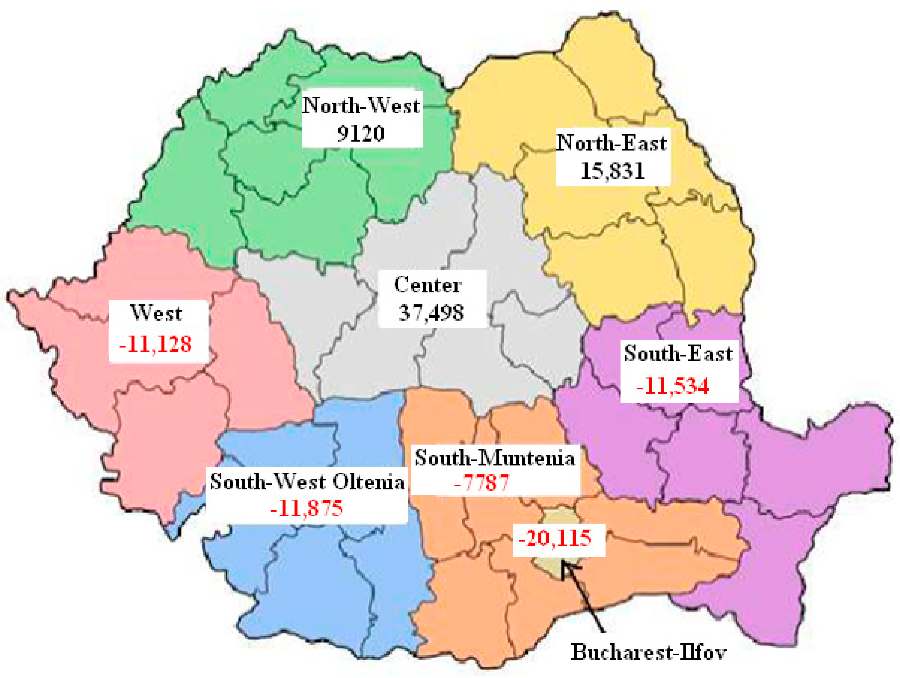
| Fixed Effects (Cross) | ||||
| _NV--C | 9120.251 | |||
| _CE--C | 37498.26 | |||
| _NE--C | 15831.54 | |||
| _SE--C | −11543.02 | |||
| _SM--C | −7787.306 | |||
| _BI--C | −20115.99 | |||
| _SV--C | −11875.66 | |||
| _VE--C | −11128.09 | |||
| Fixed Effects (Period) | ||||
| 2004--C | −10047.28 | |||
| 2005--C | 7200.238 | |||
| 2006--C | −2974.132 | |||
| 2007--C | 3955.534 | |||
| 2008--C | 9231.927 | |||
| 2009--C | −15320.37 | |||
| 2010--C | −16160.52 | |||
| 2011--C | 8814.043 | |||
| 2012--C | 15300.56 | |||
| Effects Specification | ||||
| Cross-section fixed (dummy variables) | ||||
| Period fixed (dummy variables) | ||||
| R-squared | 0.955780 | Mean dependent var | 75105.10 | |
| Adjusted R-squared | 0.941859 | S.D. dependent var | 73379.15 | |
| Sum squared resid | 1.69 × 10¹⁰ | Akaike info criterion | 22.61211 | |
| Log likelihood | −796.0359 | Schwarz criterion | 23.18127 | |
| F-statistic | 68.65650 | Hannan-Quinn criter. | 22.83870 | |
| Prob(F-statistic) | 0.000000 | Durbin-Watson stat | 1.645208 | |
Notes: Dependent Variable: OS; Method: Pooled Least Squares; Sample (adjusted): 2004, 2012; Included observations: 9 after adjustments; Cross-sections included: 8; Total pool (balanced) observations: 72.
The values of the determination ratio, R-squared = 0.955780, and of the F-statistic = 0.955780, which corresponds to an insignificant probability of error, Probability(F-statistic) = 0.00, lead to the conclusion that the model is valid, and the dependencies between the variables OS and GDP in the eight regions developed in Romania during 2004–2012 are well approximated. Consequently, the model can be used to estimate the evolution of overnight stays by GDP evolutions.
Coefficients a0(22,411.05), a1(0.819036) and a2(0.094438) are significantly different from zero, as shown in Table 6, and the corresponding variables OS(−1) and d(GDP(−1)) are statistically significant for a probability of error of less than 1% even for a bilateral t test. Regarding the coefficient C (constant term a0), it is statistically significant for a bilateral t test for a probability of 90%.
However, given that the test used to test the validity of model coefficients is a t-Student unilateral test, where t-statistic = 1.812230 corresponds to a probability of error of 3.77%, it can be said, with a 95% probability, that the panel is homogeneous, which means that in all development regions there are common elements in time and space, which explains the dynamics of the OS variable, over which regional specific effects overlap.
At a general level, considering the coefficients a1 and a2 what results is, on the one hand, that the evolution of changes in the volume of the GDP, expressed in the variable factor d(GDP) directly influences, in the same sense, evolutions of overnight stays in the agrotouristic boarding houses, in a proportion of 9.44% (a2 = 0.094438); on the other hand, it forms a positive feedback loop between overnight stays (OS) in two consecutive years; the value of the dependent variable OS in the current year depends on its value in the previous year, the influence being significant (a1 = 0.819036).
Above this general trend, the individual effects of each region overlap. The data from Table 6 and Figure 1 show that, in the North-West, North-East and Central regions, the level of overnight stays in agrotouristic boarding houses exceeds the average, the higher correction corresponding to the Central region (37,498.26), which means that the pressure of this kind of tourism on sustainability in its counties is much higher.
Figure 1.
The effects of the specificity of regions on OS.
In the other five development regions, specific effects manifest in reverse. The evolutions of the number of overnight stays in agrotouristic boarding houses are lower compared to the average. A significant decrease was recorded in South-West Oltenia, the South-East and the West, which means that the pressure of rural tourism on sustainability in this region is much lower.
Regarding the Bucharest-Ilfov development region, although the specific correction is −20,115.99, here the pollution and environmental degradation are caused mainly by the urban agglomeration, by the very large number of motor vehicles and by some of the existing commercial and industrial complexes.
Analyzing the temporal effects, we see that corrections are generally positive. However, the corresponding values of 2009 (−15,320.37) and 2010 (−16,160.52) are worth mentioning, as they highlight the effects of the economic crisis on rural tourism in Romania. Since 2011, values which highlight favorable circumstances have been recorded.
4. Conclusions
The particularities of rural tourism developed in the context of sustainable development are generated by multiple cultural features, biological diversity and the ecological capital as a whole. These must be preserved, along with the need to develop local economies in order to increase the living standards of rural residents.
In Romania, due to the cultural diversity determined by specific traditions inherited over the centuries, and due to the natural heritage of the eight regions, the studies concerning ways of conducting sustainable rural tourism involve approaches, if not punctual, at least at a regional level. On the other hand, we must take into account the fact that this form of tourism has evolved differently over the last decade and therefore the pressures on the sustainable development of counties and local communities are different.
Given the density of rural tourism traffic in the last decade in the eight development regions of Romania, the general trend on the development of rural tourism was highlighted using an econometric model based on panel data series, and quantitative assessments that differentiate development regions from one another were made as well.
Although, at the country level, in Romania rural tourism is a form of tourism which has increasingly drawn more interest, both from Romanian citizens and from foreigners, the analysis of the results shows significant differences between the eight development regions of Romania. In the Central development region, which includes counties from the heart of Transylvania (Alba, Brasov, Covasna, Harghita, Mures and Sibiu) tourist flows are significantly higher than in the other development regions, the Cross Effects having values two times higher than the next ranked. Although the results obtained in the development of the road infrastructure that ensures access to this region are relatively modest, the natural and anthropogenic potential of the counties highlights a good preservation of the medieval age sights (fortified churches, fortresses Fagaras, Alba-Iulia, Bran and others) and the existence of rural civilization areas that have been preserved unchanged, such as the area Viscri, all of these being significant tourist attractions. However, on the other hand, the tourist flows urge the adoption of immediate measures to ensure sustainability.
The North-East Region, comprising the counties of Northern Moldavia, of which Neamt, Suceava and Iasi have a special historical significance, and which, through its monasteries, is an important attraction for religious tourism, also records significant rural tourist flows. Although the natural and anthropogenic potential of this region is no less than that of the Central region, the road infrastructure linking this region with Central and Western Europe is relatively poor, significantly limiting tourist access.
A third region, which has positive values of the Fixed Effects Cross indicator, is the North-West development region, which includes the counties of Bihor, Bistrita-Năsăud, Cluj, Maramures, Satu Mare and Salaj. Among the factors leading to the recording of major tourist flows in this region, there is the proximity of the western border of Romania, which facilitates the access of foreign tourists who use road transport, as well as the particularly rich tourist supply from the Maramures, Cluj and Bistrita-Năsăud counties.
The other five development regions were characterized, in the period under review, by tourist flows that were below the average of the country level. Among these, a special situation is registered in Bucharest-Ilfov, where rural tourism is less developed because of the specificity of this area.
The South-Muntenia region is characterized by significant differences between counties in terms of their rural tourism. Thus, while Prahova, Arges and the north of Dâmboviţa have developed both mountain tourism and rural tourism, counties such as Calarasi, Ialomita, Giurgiu, Teleorman and a large part of Dâmboviţa are plain counties, where tourism is relatively limited, and in which, due to the decline of agriculture that led to a low standard of living, rural tourism offer is quite limited.
Although the tourism offers of the counties of Constanta (the Black Sea) and Tulcea (the Danube Delta) are significant, the attracted tourist flows do not compensate those of the other counties of the South-East development region. An increase in the density of tourist flows in this region, in the fishing villages and the Black Sea villages, can be obtained by the construction of at least a fast road between Pitesti and Sibiu to link the sectors of the A1 and the A2 motorways.
Similar situations are found in the developing regions of West and South-West Oltenia. Within these, although there are areas with special natural and anthropic potential, the relatively weak promotion measures, on the one hand, and poor maintenance of some traditional tourist areas (Baile Herculane), on the other hand, negatively influence the density of rural tourism flows.
Based on these findings, the future research directions will aim at the determination of the specific values of indicators that characterize the aggregate Statistical System at the level of each county. Also, this being given, we aim to identify their similarities and particularities, in order to define an aggregate system at the level of each development region.
Acknowledgments
This paper has been financially supported within the project entitled “Horizon 2020—Doctoral and Postdoctoral Studies: Promoting the National Interest through Excellence, Competitiveness and Responsibility in the Field of Romanian Fundamental and Applied Scientific Research”, contract number POSDRU/159/1.5/S/140106. This project is co-financed by European Social Fund through Sectoral Operational Programme for Human Resources Development 2007–2013. All the authors gratefully thank the reviewers and editors.
Author Contributions
Daniela Ruxandra Andrei and Rodica-Manuela Gogonea has designed the research methodology and carried out the calculus involving econometric tools and instruments. Marian Zaharia and Jean-Vasile Andrei have written the literature review, also they contributing in analyzing and debating results. All the authors has read, approved and submitted the paper.
Conflicts of Interest
The authors declare no conflict of interest.
References
- Aall, C. Sustainable tourism in practice: Promoting or perverting the quest for a sustainable development? Sustainability 2014, 6, 2562–2583. [Google Scholar] [CrossRef]
- Moscardo, G.; Murphy, L. There is no such thing as sustainable tourism: Re-conceptualizing tourism as a tool for sustainability. Sustainability 2014, 6, 2538–2561. [Google Scholar] [CrossRef]
- Andrei, D.R.; Sandu, M.; Gogonea, R.M.; Chiriţescu, V.; Kruzslicika, M. Modeling of rural tourism towards sustainable development from the perspective of specifically organic food. Sci. Pap. Ser. Manag. Econ. Eng. Agric. Rural Dev. 2012, 12, 21–28. [Google Scholar]
- Rodriguez, L.G.; Perez, M.R.; Yang, X.; Geriletu. From Farm to Rural Hostel: New Opportunities and Challenges Associated with Tourism Expansion in Daxi, a Village in Anji County, Zhejiang, China. Sustainability 2011, 3, 306–321. [Google Scholar] [CrossRef]
- Gao, S.; Huang, S.; Huang, Y. Rural tourism development in China. Int. J. Tour. Res. 2009, 11, 439–450. [Google Scholar] [CrossRef]
- Ailenei, D.; Jula, D. Diminuarea Inegalităţilor Condiţie Esenţială a Coeziunii Economice şi Sociale. Available online: http://coeziune.ase.ro/files/Sinteza.pdf (accessed on 14 July 2014). (In Romanian)
- Daly, H.E.; Cobb, J.B., Jr. For the Common Good: Redirecting the Economy towards the Community, the Environment and a Sustainable Future; Greenprint: London, UK, 1990. [Google Scholar]
- Pearce, D.W.; Warford, J.J. World without End. Economics, Environment, and Sustainable Development; Oxford University Press: Oxford, UK, 1993. [Google Scholar]
- Done, I.; Chivu, L.; Andrei, J.; Matei, M. Using labor force and green investments in valuing the Romanian agriculture potential. J. Food Agric. Environ. 2012, 10, 737–741. [Google Scholar]
- Mebratu, D. Sustainability and sustainable development: Historical and conceptual review. Environ. Impact Assess. Rev. 1998, 18, 493–520. [Google Scholar] [CrossRef]
- Bartelmus, P. Dematerialization and Capital Maintenance: Two Sides of the Same Coin. Ecol. Econ. 2003, 46, 61–88. [Google Scholar] [CrossRef]
- Common, M.; Stagl, S. Ecological Economics. An Introduction; Cambridge University: Cambridge, UK, 2005. [Google Scholar]
- Hamilton, K.; Withagen, C. Savings growth and the path of utility. Can. J. Econ. 2007, 40, 703–713. [Google Scholar] [CrossRef]
- Popescu, G.; Andrei, J. From industrial holdings to subsistence farms in the Romanian agriculture. Analyzing the subsistence components of the CAP. Zemedelska Ekonomika 2011, 57, 555–564. [Google Scholar]
- Ruta, G.; Hamilton, K. The Capital Approach to Sustainability. In Handbook of Sustainable Development; Atkinson, G., Dietz, S., Neumayer, E., Eds.; Edward Elgar Publishing Inc.: Cheltenham, UK, 2007. [Google Scholar]
- Eurostat. GDP and main components—Current prices. Available online: http://epp.eurostat.ec.europa.eu/portal/page/portal/statistics/search_database (accessed on 30 September 2014).
- Walpole, M.J.; Goodwin, H.J. Local attitudes towards conservation and tourism around Komodo national park, Indonesia. Environ. Conserv. 2002, 28, 160–166. [Google Scholar]
- Mehta, J.N.; Kellert, S.R. Local attitudes toward community-based conservation policy and programs in Nepal: A case study in the Makalu-barun conservation area. Environ. Conserv. 1998, 25, 320–333. [Google Scholar] [CrossRef]
- Walpole, M.J.; Goodwin, H.J. Local economic impacts of dragon tourism in Indonesia. Annal. Tour. Res. 2000, 27, 559–576. [Google Scholar] [CrossRef]
- European Commission. Statistics Explained, Rural Development Statistics by Urban-Rural Typology. Available online: http://epp.eurostat.ec.europa.eu/statistics_explained/index.php/Rural_development_statistics_by_urban-rural_typology (accessed on 14 July 2014).
- Emptaz-Collomb, J.-G.J. Linking Tourism, Human Wellbeing and Conservation in the Caprivi Strip (Namibia); University of Florida: Gainesville, FL, USA, 2009. [Google Scholar]
- Baltagi, B.H. Econometric Analysis of Panel Data; John Wiley & Sons Ltd.: West Sussex, UK, 2005. [Google Scholar]
- European Commission. Towards Quality Rural Tourism. Available online: http://ec.europa.eu/enterprise/sectors/tourism/files/studies/towards_quality_tourism_rural_urban_coastal/iqm_rural_en.pdf (accessed on 16 July 2014).
- Hsiao, C. Analysis of Panel Data, 2nd ed.; Cambridge University Press: Cambridge, UK, 2003. [Google Scholar]
- Toda, H.Y.; Yamamoto, T. Statistical inference in Vector Autoregressions with possibly integrated processes. J. Econ. 1995, 66, 225–250. [Google Scholar] [CrossRef]
- Gogonea, R.M.; Zaharia, M. Econometrie cu Aplicaţii în Activitatea de Comerţ-Turism-Servicii; Editura Universitară: Bucureşti, Romania, 2008. (In Romanian) [Google Scholar]
- Granger, C.W.J. Investigating Causal Relations by Econometric Models and Cross-spectral Methods. Econometrica 1969, 37, 424–438. [Google Scholar] [CrossRef]
- Granger, C.W.J. Time Series Analysis, Cointegration, and Applications. Am. Econ. Rev. 2004, 94, 421–425. [Google Scholar] [CrossRef]
© 2014 by the authors; licensee MDPI, Basel, Switzerland. This article is an open access article distributed under the terms and conditions of the Creative Commons Attribution license (http://creativecommons.org/licenses/by/4.0/).