Abstract
This paper evaluates the possible impacts of climate change and land use change and its combined effects on soil loss and net soil loss (erosion and deposition) in the Mae Nam Nan sub-catchment, Thailand. Future climate from two general circulation models (GCMs) and a regional circulation model (RCM) consisting of HadCM3, NCAR CSSM3 and PRECIS RCM ware downscaled using a delta change approach. Cellular Automata/Markov (CA_Markov) model was used to characterize future land use. Soil loss modeling using Revised Universal Soil Loss Equation (RUSLE) and sedimentation modeling in Idrisi software were employed to estimate soil loss and net soil loss under direct impact (climate change), indirect impact (land use change) and full range of impact (climate and land use change) to generate results at a 10 year interval between 2020 and 2040. Results indicate that soil erosion and deposition increase or decrease, depending on which climate and land use scenarios are considered. The potential for climate change to increase soil loss rate, soil erosion and deposition in future periods was established, whereas considerable decreases in erosion are projected when land use is increased from baseline periods. The combined climate and land use change analysis revealed that land use planning could be adopted to mitigate soil erosion and deposition in the future, in conjunction with the projected direct impact of climate change.
1. Introduction
Soil erosion is a major environmental threat to the sustainability and productive capacity of agriculture [1,2]. It is considered as one of the major land degradation processes in the Upper Nan watershed, Thailand, which is also the main source of environmental deterioration [3]. Soil loss creates negative impacts on agricultural production [4] of crops such as corn and soybeans, infrastructure and water quality. The potential causes of increased soil erosion could be increased temperatures, altered precipitation patterns (strength, timing and altitude), changes in snow cover and seasonal snow melting caused by climate change [5]. Climate change is expected to affect soil erosion based on a variety of factors [6] including precipitation amount and intensity impacts on soil moisture and plant growth, and direct fertilization effects on plants due to greater CO2 concentrations among others. Many studies have shown that climate change could significantly affect soil erosion [7,8,9,10,11]. The most direct impact of climate change on soil erosion is the change in the erosive power of rainfall [9,10,11,12,13]. The contribution of water as an erosion agent can be represented by rainfall erosivity (R-factor). This factor may be the most important and dominant in the Universal Soil Loss Equation (USLE) [14] and the Revised Universal Soil Loss Equation (RUSLE) [15]. Both are sets of mathematical equations that estimate average annual soil loss from interrill and rill erosion [16]. Rainfall is the driving force affecting the energy balance of the soil erosion process [17]. The erosivity of rainfall and its consecutive overland runoff is recognized as a crucial factor for erosion processes [18]. Rainfall erosivity is described as the average annual sum of EI30 determined from rainfall records.
Global changes in temperature and precipitation patterns will impact soil erosion through multiple pathways, including precipitation and rainfall erosivity changes [19]. Climate change is expected to affect soil erosion based on a variety of factors, including precipitation amounts and intensities, temperature impacts on soil moisture and plant growth [20]. The erosive power of rainfall has a direct impact on soil loss. Current general circulation models (GCMs) and regional climate models (RCMs) [20,21] cannot furnish detailed precipitation information that enables the computation of the rainfall erosivity directly as a function of rainfall kinetic energy and rainfall intensity. Hence, the precipitation and rainfall erosivity relationship was established on the basis of the GCMs/RCMs output [20,22].
Land use/land cover (LULC) is defined as the observed physical layer including natural and planted vegetation and human constructions. The reduction of vegetation cover can increase soil erosion. This relationship is the reason why vegetation cover and land use have been widely included in soil erosion studies [23,24,25,26,27,28]. Previous studies have found that land use can greatly affect the intensity of runoff and soil erosion [24,29,30]. Vegetation controls soil erosion by means of its canopy, roots and litter components. Erosion also influences vegetation in terms of the composition, structure and growth pattern of the plant community [31]. Therefore, the modeling of land use change is important with respect to the prediction of soil erosion.
Most previous studies concerning soil loss have been based on the USLE/RUSLE [14,15]. It is one of the most commonly applied models to estimate soil erosion [32,33,34], although RUSLE was developed to be applied to one dimensional hill slopes which do not examine the related process of deposition [15,35] and, thus, RUSLE’s conceptualization only permits soil loss to be estimated. One of the limitations of the RUSLE model is that it cannot estimate deposition. Thus, static assessments of soil losses were used as inputs into an algorithm of deposition in a sedimentation model that models the movement of sediment to the outlet. The sedimentation model is based on the results of the RUSLE model to calculate the balance of erosion in each elementary plot considered homogeneous. Some authors have asserted the possibility of identifying deposition zones using accurate DEMs [36,37]. Many studies [34,37,38] have extended RUSLE to also estimate sediment yield. The approach presented here directly integrates RUSLE’s output data into a flow model, which allows soil loss rate, erosion and deposition to be accessed within a GIS framework without additional data requirements. In addition, a number of studies have integrated geographic information system (GIS) analysis with soil erosion modeling for various geographic locations [39,40,41,42,43]. Remote sensing has proved to be a useful, inexpensive and effective tool in LULC mapping and LULC change detection. It can provide the data necessary for erosion modeling within a GIS. Given the complex nature of the erosion process, and the challenges of quantifying these processes, an integrated RS, GIS and modeling based approach is critical for the successful evaluation of the impact of land use change on land resources.
The main objective of this paper is to evaluate the simulated impacts of possible future climate, land use change and full range of impacts (climate and land use change) on the soil erosion and deposition in the Mae Nam Nan sub-catchment in Thailand.
2. Site Description
2.1. Study Area
The Upper Nan watershed is located in northern Thailand. More than 85% of the watershed is mountainous, and the rate of soil erosion in the area by average is higher than 200 Mg ha−1 yr−1 (Figure 1) which is the highest among watersheds in the north Thailand (LDD 2000). The study area, the Mae Nam Nan sub-catchment is located in the Upper Nan watershed, and the area is about 1532 km2. The topography of study area ranges from flat terrain to mountains, with an elevation of 120 to 1900 meters above mean sea level (Figure 2), and the percentage of covered area is different for the slope categories as follow: horizontal (0%–2% slope) cover 19.51%; very flat (2%–5% slope) cover 24.03%; flat slope (5%–10% slope) cover 22.04%; moderate (10%–25% slope) cover 25.99% and steep slope (>25% slope) cover 8.43% of area (Figure 2). The land use consists mainly of degraded forest and upland agriculture such as paddy field, orchard, upland crop, maize, and vegetables grown in both shifting and permanent cultivation patterns [44].
2.2. Geology and Soil Type
The geology of the Mae Nam Nan sub-catchment comprises various kinds of rocks and rock units ranging in age from the Carboniferous. The study area consists mainly of Paleozoic and Mesozoic sedimentary rocks and Mesozoic Igneous rocks. Paleozoic rocks ranging from Carboniferous rocks consist mainly of sandstone and shale, Permian rocks consist mainly of limestone sandstone and shale, Silurian Devonian rocks consist of Phyllite, Quartzite, Schist and greywacke locally, Mesozoic rocks consist of conglomerate, sandstone and siltstone. The soils formed on low-lying landscape are mostly young loamy soils and are classified as Alluvial soils. They are relatively fertile soils and mainly used for rice cultivation or upland and tree crops [44,45]. Soils formed in the area vary widely in depth, texture, color, fertility as well as in their agricultural potential depending largely upon the kind of parent rock of each soil.
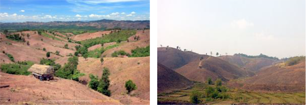
Figure 1.
Land degradation by soil erosion in the Mea Nam Nan sub-catchment. (Picture by Pheerawat Plangoen in April 2013.)
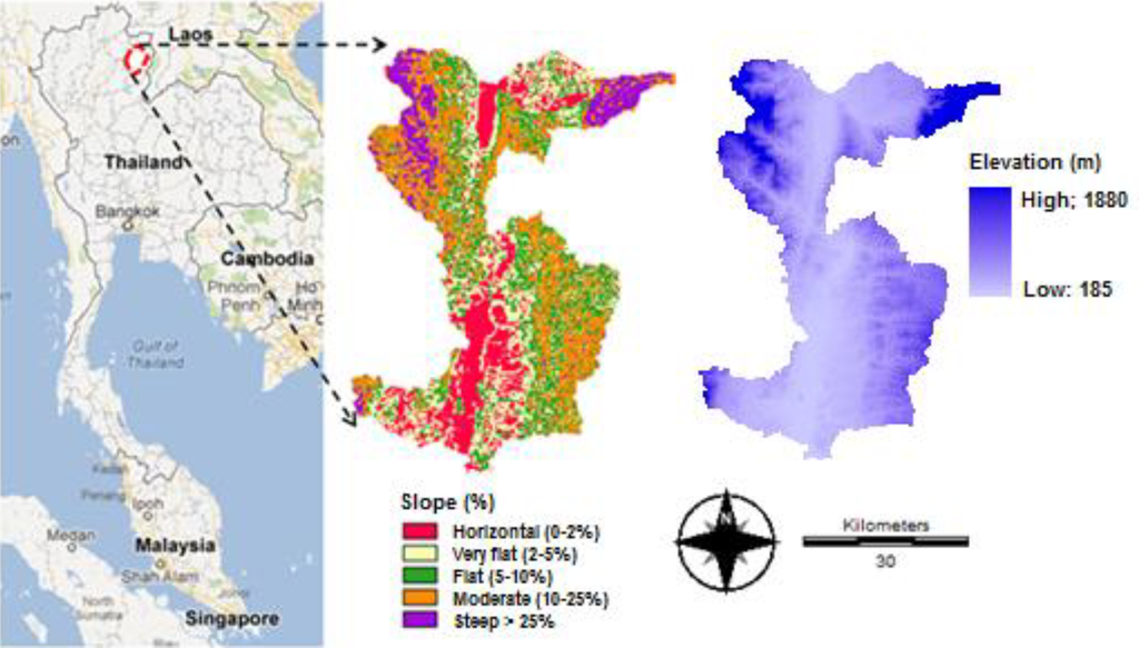
Figure 2.
Location of study area, using images from Google maps.
2.3. Climate
The general climate of the study area is tropical monsoon and characterized by winter, summer and rainy season, influenced by the northeast and southwest monsoons. The rainy season brought about by the southwest monsoon originating from the Indian Ocean lasts from mid-May until the end of October. July and August are usually months of intense rainfall. During the winter season, the weather is cold and dry due to the northeast monsoons beginning in November and ending in February. From mid-February until mid-May, the weather is rather warm. The annual rainfall is about 1,263 mm. More than 80 percent of the rainfall is concentrated in the wet season.
3. Methodology
3.1. Soil Loss Modeling
The Revised Universal Soil Loss Equation (RUSLE) [15] module was integrated into the GIS Idrisi. This module not only calculates soil losses for each pixel of the grid but also for groups of pixels into homogeneous polygons, based on the slope criteria, orientation and slope length which can be adjusted by the user [46]. The RUSLE equation model is as follows:
Where: A is the computed soil loss per unit area, (Mg ha−1 y−1), R is the rainfall erosivity factor (MJ mm ha−1 y−1), K is the soil erodibility factor (tons ha MJ−1 mm−1), is the soil loss rate per erosion index unit for a specified soil as measured on a unit plot, L is the slope-length factor, S is the slope-steepness factor, C is the cover and management factor and P is the support practice factor.
A = R K L S C P
3.2. Sedimentation Modeling
The sedimentation model is based on the results of the RUSLE model to determine the balance of erosion in each elementary patch and evaluate the net movement of soil (erosion or deposition) in sub catchment [39]. One of limitations of the RUSLE model is that its application to any land unit must result in soil loss but it cannot estimate deposition. However, within agricultural areas and river basins, deposition occurs. The down slope movement of soil loss from one field to another is not conceptualized within RUSLE. Net erosion or deposition for a given area is calculated in the following manner when applying the sedimentation model (Figure 3), determination of patch soil loss, establishment of direction of soil movement and calculation of relative soil loss for the higher patch is compared to the soil loss for the lower patch. The difference between the amounts of soil loss from the higher patch to the lower patch represents the net soil loss or deposition in the lower patch. For example in Figure 4, if in the initial state the proportional soil loss in Patch A (the higher patch) delivered to the lower patch B is 8 t/yr, and Patch B’s initial soil loss is 12 t/yr (RUSLE soil loss value), sedimentation then determines the difference between the amount of sediment coming into the patch and the patch’s RUSLE soil loss value.
3.3. Determination of RUSLE Input Parameters
3.3.1. Soil Erodibility (K-factor)
The soil erodibility (K-factor) estimation method recommended by Wischmeier et al. [14] is most frequently used [36]. The K factor (Table 1) values were determined by Land Development Department, LDD [44] using results from laboratory analyses of soil texture, soil structure, organic matter, content and soil permeability. In the slope complex areas where the soil texture data is unavailable the K-factor based on geological formations as identified by LDD [44] was applied in this study.
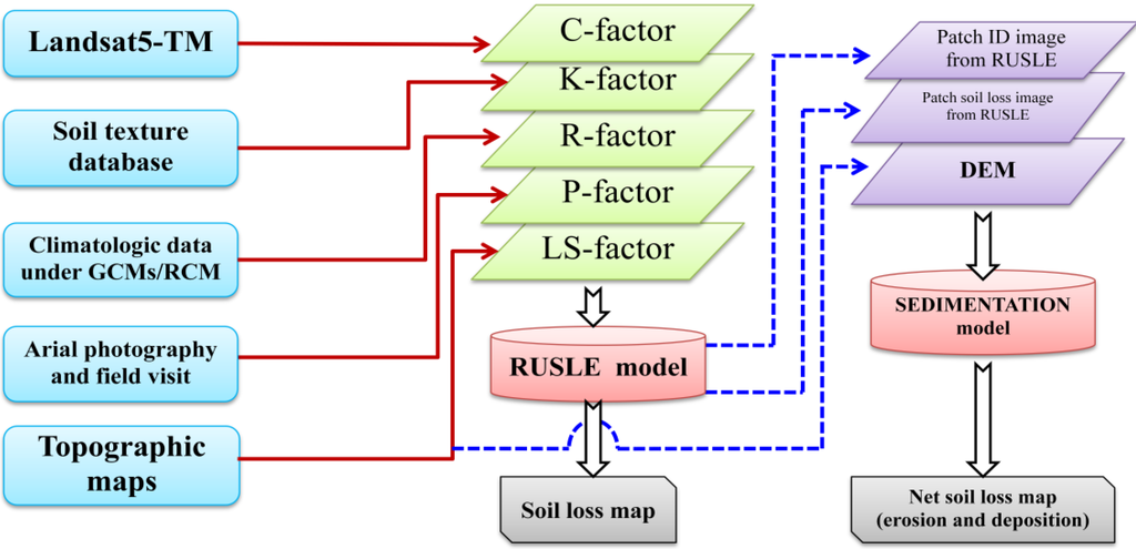
Figure 3.
Schematic chart of soil loss and net soil loss assessment.
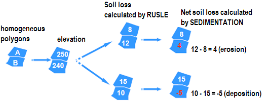
Figure 4.
Principle model of deposition: Sedimentation [47].
3.3.2. Topographic Factors (LS-factor)
To prepare the LS-factor layer, an L factor and S factor was generated from a digital elevation model and input the Digital Elevation Model (DEM) in the RUSLE module. The following procedures are taken in the calculation of the LS factors. The equation developed by Wischmeier and Smith [14] for this approach is as follows:
Where LS is the slope length and steepness factor, s is the field slope in percent, l is the slope length in meters, and m is the dimensionless exponential.
LS = (l/22.13)m (0.43 + 0.30s + 0.043s2)/6.574

Table 1.
Attribute values of the soil erodibility (K factor, tons h MJ−1 mm−1).
| Textural class | K-factor | Geological formations | K-factor | ||
|---|---|---|---|---|---|
| Clay | C(low) | 0.015 | Phu Kradung | Jpk | 0.029 |
| C(up) | 0.024 | Phra Wihan Form | Jpw | 0.029 | |
| Clay | CL(up) | 0.024 | Sao Khua Form | Jsk | 0.029 |
| Loam | L(low) | 0.026 | Phu Phan Form | Kpp | 0.029 |
| L(up) | 0.024 | Nam Duk Form., | Pnd | 0.013 | |
| Loamy | LS(low) | 0.026 | Pha Nok Khao Form | Ppn | 0.013 |
| LS(up) | 0.024 | Huai Hin Lat Form | TRhl | 0.029 | |
| Sandy Clay Loam | SCL(low) | 0.026 | Nam Phong Form | TRnp | 0.024 |
| SCL(up) | 0.024 | Urban area | U | 0 | |
| Silty Clay | SiC(low) | 0.015 | Water body | W | 0 |
| Silty Clay Loam | SiCL(low) | 0.035 | |||
| SiCL(up) | 0.025 | ||||
| Silty Loam | SiL(up) | 0.025 | |||
| Sandy Loam | SL(up) | 0.024 | |||
3.3.3. Rainfall Erosivity (R-factor)
The concept of rainfall erosivity refers to the ability of any rainfall event to erode soil. The rainfall erosivity is defined as the average annual value of the rainfall erosion index [48]. The monthly rainfall erosivity value was computed by summing up EI30 values of storms that occurred during the month [49]. The RUSLE model uses the Brown and Foster [50] approach for calculating the average annual rainfall erosivity, R (MJ mm ha−1 h−1 y−1)
 where E is the total storm kinetic energy (MJ ha−1), I30 is the maximum 30 minute rainfall intensity (mm h−1), j is an index of the number of years used to produce the average, k is an index of the number of storms in each year, n is the number of years used to obtain the average R, and m is the number of storms in each year.
The total storm kinetic energy (E) is determined using the relation,
 where er is the rainfall energy per unit depth of rainfall per unit area in megajoules per hectare per millimeter (MJ ha−1 mm−1), and ∆Vr is the depth of rainfall in millimeters (mm) for the rth increment of the storm hyetograph which is divided into m parts, in which each part has a constant rainfall value.
Rainfall energy per unit depth of rainfall (er) can be calculated using the relation:
where er has units of megajoules per hectare per millimeter of rain (MJ ha−1 mm−1), and ir is rainfall intensity (mm h−1). Rainfall intensity for a particular increment of a rainfall event (ir) is calculated using the relation.
 where ∆tr is the depth of rain falling (mm) during the increment.
er = 0.29[1 – 0.72 exp( –0.05 ir)]
Estimation of the annual rainfall erosivity using the modified Fournier index (MFI) has been proposed when only monthly precipitation data are available [51].
 where pi is the mean monthly rainfall of the month i, P is the mean annual rainfall
The relationship between MFI and the R factor showed better adjustment following an exponential distribution [52]. The R factor values can be estimated from the MFI using the following equation.
where a and b are empirical parameters and ε is a random, normally distributed error.
R = aMFIb + ε
Estimation of future climate change provided by Global Circulation Models (GCMs) and RCM do not provide the type of detailed storm information needed to directly calculate predicted R factor changes. Therefore, statistical relationships between monthly precipitation and modified Fournier index (MFI), and MFI versus rainfall erosivity were used to analyze the GCMs/RCMs outputs relative to R factor changes [53] in order to analyze the spatial distribution of rainfall erosivity under future climate. R factor values were calculated using the method described by Renard (1997) [15]. For the study, the commonly used HadCM3, CCSM3 and PRECIS RCM were chosen to generate the future precipitation scenarios.
3.3.4. General Circulation Models
For this study two GCMs were selected on the basis of their performance in the simulation of precipitation. (1) The NCAR’s Community Climate System Model (CCSM3) was one of the global climate models included in the Fourth Assessment Report (AR4) of the Intergovernmental Panel on Climate Change (IPCC). NCAR’s GIS program provides GIS-compatible user access to CCSM3 AR4 global (1.4 degree or 155 km). The selected GCMs were downloaded from the NCAR community climate system model (CCSM) projections in GIS format, available at [54]. (2) HadCM3 was used to generatethe future precipitation scenarios. HadCM3 is a coupled atmospheric-ocean GCM developed at the Hadley Centre of the United Kingdom National Meteorological Service that studies climate variability and change. The atmospheric component of the model has 19 levels with a horizontal resolution of 2.5° latitude and 3.75° longitude. The ocean component of the model has 20 levels with horizontal resolution 1.25° latitude 1.25° longitude.
3.3.5. Regional Climate Model
The RCM used in this study was PRECIS, developed by the Hadley Centre of the UK Meteorological Office. The PRECIS RCM is based on the atmospheric components of the ECHAM4 GCM from the Max Planck Institute for Meteorology, Germany. The PRECIS data are produced by the Southeast Asian System for Analysis, Research and Training (SEA START) Regional Center for 2225 grid cells covering the entire Mae Nam Nan Sub-Catchment with the resolution of 0.2 × 0.2 degree (approximately 22 × 22 km2). These data comprise two data sets for ECHAM4 SRES A2 and B2, daily precipitation. The PRECIS RCM data over the periods of 1971–2000 (present) and 2011–2098 (future), for both A2 and B2 scenarios, were obtained from the Southeast Asian START Regional Center [55].
Several statistical downscaling techniques have been developed to translate large-scale GCM/RCM output into finer resolution [56]. In this study, the simplest method change factor or delta change approach was applied. The change factor or delta change method has been used in many earlier climate change impact studies [57,58,59,60,61]. Basically, this approach modifies the observed historical time series of precipitation and is modified by multiplying the ratio of the monthly future and historic precipitations simulated by NCAR CCSM3 (A2, A1b and B1 scenarios), HadCM3 and PRECIS RCM (A2 and B2 scenarios) for each time period. The observational database used for this approach covers the period of 1981–2000.
3.3.6. Cover Management Factor (C factor)
The cover management (C factor) reflects the effect of cropping on the soil erosion rate [15]. The crop and management factors (C-factor) corresponding to each crop/vegetation condition were estimated from the RUSLE guide. In this study, the LULC maps were derived from the satellite images and served as a guiding tool in the allocation of C factor for different land use classes, and the values set by LDD [62] for the various vegetation cover types as show in Table 2. The C factor in future was converted from LULC as the result of CA_Markov model.
Table 2.
Attribute values of vegetative cover (C factor) [62].
| Land cover class | C Value |
|---|---|
| Paddy field | 0.28 |
| Upland crop | 0.6 |
| Orchard | 0.15 |
| Forest | |
| Dry evergreen forest | 0.019 |
| Deciduous Dipterocarp Forest | 0.048 |
| Mixed Deciduous Forest | 0.048 |
| Forest plantation | 0.088 |
| Urban | 0 |
| Water body | 0 |
The CA_Markov model [63] was used to perform land use change analysis between 1990 and 2000, 2000 and 2010 LULC. CA_Markov is a combined Cellular Automata, Markov Chain and Multi-Criteria/Multi-Objective Land Allocation (MOLA) land cover prediction procedure that adds an element of spatial contiguity as well as knowledge of the likely spatial distribution of transitions to Markov chain analysis. Therefore, the predicting land use/land cover in 2010 (based on land cover data in 1990 and 2000) and 2020, 2030 and 2040 (based on land cover data in 2000 and 2010).
3.3.7. Conservation Practice Factor (P-factor)
The support practice factor is the soil loss ratio with a specific support practice to the corresponding soil loss with up-and-down slope tillage. Table 3 shows the P factor values for three major support practices in cultivated lands as given by Wischmeier and Smith (1978) [14]. Conservation practices are not common in Thailand, the values for the P-factor have not been fully established for all vegetation cover types, the exception being for paddy fields. Thus, values of “0.1” and “1” are assigned to paddy fields and other land cover types, respectively [36].
Table 3.
Support practice factor P for cultivated lands [14].
| Land slope % | Contouring | Contour, strip cropping, and irrigated furrows | Terracing |
|---|---|---|---|
| 1–2 | 0.60 | 0.30 | 0.12 |
| 3–8 | 0.50 | 0.25 | 0.10 |
| 9–12 | 0.60 | 0.30 | 0.12 |
| 13–16 | 0.17 | 0.35 | 0.14 |
| 17–20 | 0.80 | 0.40 | 0.16 |
| 21–25 | 0.90 | 0.45 | 0.18 |
3.3.8. Validation of the RUSLE to Study Area.
The RUSLE is validated for the study area using experimental plots located in the Upper Nan watershed at Nan Watershed Research Station, Nan Province and was carried out in 1992. There are a total of 14 experimental plots in the previous study [64] having various types of land use. Experimental plots have a length of 20 m and width of 4 m [65] with a 17.5 percent slope at an elevation of 500 m above mean sea level. Other parameters such as soil erodibiltiy factor from nomograph including soil erodibility factor from up and down hill continuous fallow on bare soil plots were also computed. Measured soil loss data of 36 rainfall events from April to October 1992 were collected from testing and validating plots. The descriptive statistics testing includes average error (AE), relative error (RE), and standard error (SE), and can be calculated by the following equations [65,66,67]:

 where Ci,m is the soil loss (ton ha−1) from the model estimation rainfall event i, Ci,a is the soil loss (ton ha−1) from the actual experimental plot rainfall event i, n is the total amount of rainfall event on the sample, and Cmean,a is the mean soil loss (ton ha−1) from the experimental plot.
4. Results
4.1. Image Classification and Accuracy Assessment
The result of accuracy of land cover classification will be discussed based on an Error/Confusion matrix. Table 4 shows an overall classification accuracy of 86% and the overall Kappa statistics of 0.83, which is on the border of a good classification performance. High and low producer accuracies were observed in water body and forest (100% and 77%). High and low user’s accuracies were observed in upland crop and urban area (92% and 76%). For Table 5, Table 6, overall accuracies for the maps of 2000 and 2010 were 81% and 83% with an overall kappa statistics of 0.77 and 0.79, respectively. It is noted that a minimum accuracy value of 80% [30] is required for effective and reliable land cover change analysis and modeling. The classification achieved in this study produced an overall accuracy that fulfils the minimum accuracy threshold.
Table 4.
Error matrix of land use/land cover (LULC) map obtained using 1990’s TM images.
| Land Use Type | Land use by Ground truth | Total area | User’s Accuracy (%) | ||||||
|---|---|---|---|---|---|---|---|---|---|
| A | B | C | D | E | F | ||||
| Overall accuracy = 86%, Overall Kappa = 0.83 | |||||||||
| A. Paddy field | 335 | 54 | 0 | 0 | 0 | 0 | 389 | 86 | |
| B. Upland crop | 0 | 434 | 0 | 21 | 18 | 0 | 473 | 92 | |
| C. Orchard | 0 | 0 | 242 | 51 | 0 | 0 | 293 | 83 | |
| D. Forest | 0 | 0 | 53 | 317 | 0 | 0 | 370 | 86 | |
| E. Urban | 26 | 50 | 0 | 0 | 247 | 0 | 323 | 76 | |
| F. Water body | 0 | 0 | 0 | 25 | 0 | 221 | 246 | 90 | |
| Total area | 361 | 538 | 295 | 414 | 265 | 221 | 2094 | ||
| Producer’s Accuracy (%) | 93 | 81 | 82 | 77 | 93 | 100 | |||
Table 5.
Error matrix of LULC map obtained using 2000’s TM images.
| Land Use Type | Land use by Ground truth | Total area | User’s Accuracy (%) | |||||||||
|---|---|---|---|---|---|---|---|---|---|---|---|---|
| A | B | C | D | E | F | |||||||
| Overall accuracy = 81%, Overall Kappa = 0.77 | ||||||||||||
| A. Paddy field | 435 | 62 | 0 | 22 | 11 | 16 | 546 | 80 | ||||
| B. Upland crop | 0 | 418 | 0 | 23 | 0 | 29 | 470 | 89 | ||||
| C. Orchard | 26 | 61 | 448 | 19 | 0 | 0 | 554 | 81 | ||||
| D. Forest | 52 | 0 | 0 | 499 | 62 | 92 | 705 | 71 | ||||
| E. Urban | 0 | 0 | 0 | 26 | 267 | 46 | 339 | 79 | ||||
| F. Water body | 0 | 34 | 0 | 0 | 0 | 439 | 473 | 93 | ||||
| Total area | 513 | 575 | 448 | 589 | 340 | 622 | 3087 | |||||
| Producer’s Accuracy (%) | 85 | 73 | 100 | 85 | 79 | 71 | ||||||
Table 6.
Error matrix of LULC map obtained using 2010’s TM images.
| Land Use Type | Land use by Ground truth | Total area | User’s Accuracy (%) | ||||||
|---|---|---|---|---|---|---|---|---|---|
| A | B | C | D | E | F | ||||
| Overall accuracy = 83%, Overall Kappa = 0.79 | |||||||||
| A. Paddy field | 476 | 15 | 0 | 49 | 0 | 0 | 540 | 88 | |
| B. Upland crop | 57 | 428 | 45 | 41 | 0 | 0 | 571 | 75 | |
| C. Orchard | 51 | 0 | 548 | 53 | 10 | 0 | 662 | 83 | |
| D. Forest | 29 | 0 | 0 | 422 | 76 | 0 | 547 | 80 | |
| E. Urban | 0 | 66 | 0 | 24 | 296 | 0 | 386 | 77 | |
| F. Water body | 0 | 0 | 0 | 0 | 23 | 464 | 487 | 95 | |
| Total area | 613 | 509 | 593 | 609 | 405 | 464 | 3193 | ||
| Producer’s Accuracy (%) | 78 | 84 | 92 | 72 | 73 | 100 | |||
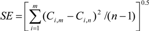
The result of LULC pattern classification from land sat images in 1990, 2000 and 2010 is shown in Figure 5. It was found that the LULC pattern in 1990 was mainly classified as 68% forest (1034 km2), followed by crops, orchards, urban, water body and paddy fields (376, 89, 17, 8 and 7 km2 respectively). The LULC pattern in 2000 was mainly classified as forest with an area of 638 km2 or 47%. Meanwhile the other included upland crops, orchards, paddy, urban areas, and water body with the areas of 452, 270, 95, 62 and 14 km2, respectively. The LULC pattern in 2010 was mainly classified as forest with an area of 724 km2 or 42% of total area. Other land use classes included upland crops, orchard, paddy, urban areas, and water body with areas of 439, 168, 119, 68 and 15 km2, respectively.
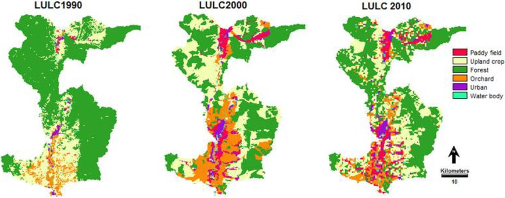
Figure 5.
LULC classification maps of the Mae Nam Nan Sub-Catchment.
4.2. The Predicted LULC in the Future Based on the Data in 2000 and 2010
The LULC data in 1990 and 2000 were operated by the Markov chain model in order to identify the probability of changing and transition areas. Such probability transition values were applied to predict the LULC for the year 2010 with a CA_Markov model. The result was the LULC map for 2010 as shown in Figure 6. The accuracy of the simulated LULC maps in the year 2010 was analyzed by comparing the LULC map with the LULC map in the year 2010 derived from the segmentation classification technique. Table 7 shows that high and low user’s accuracies of 94% and 31%, respectively, were observed in forest and water bodies. Similarly, high and low producer’s accuracy was observed in water body (87%) and upland crop (53%). The overall accuracy and overall kappa values were of 68% and 0.60, respectively. The Kappa coefficient is a measure of agreement and can be used to assess classification accuracy [45]. It is not uncommon that the kappa coefficient is low [68], giving the impression that the coefficient takes into account not only the actual agreement in the error matrix, but also the agreement of change. Table 8 and Figure 7 illustrate projected LULC for 2020, 2030 and 2040 showing that there was a dramatic decrease in forest from a base line of approximately 37%–46% in 2020–2040. However, urban areas increase significantly by 75%–78% from past to the future from 2020 to 2040.
Figure 6.
Simulated and actual land use/land cover maps for the year 2010.
Table 7.
Error matrix between simulation results and actual land use/land cover in 2010.
| Land Use Type | Actual LULC 2010 | Total area | User’s Accuracy (%) | ||||||
|---|---|---|---|---|---|---|---|---|---|
| A | B | C | D | E | F | ||||
| Overall accuracy = 67.61%, Overall Kappa = 0.6 | |||||||||
| A. Paddy field | 2517 | 2036 | 37 | 0 | 222 | 0 | 4812 | 52 | |
| B. Upland crop | 0 | 5811 | 18 | 4936 | 0 | 14 | 10,779 | 54 | |
| C. Orchard | 0 | 2891 | 2670 | 0 | 0 | 1 | 5562 | 48 | |
| D. Forest | 0 | 43 | 803 | 13,213 | 0 | 0 | 14,056 | 94 | |
| E. Urban | 0 | 228 | 555 | 0 | 1482 | 54 | 2319 | 64 | |
| F. Water body | 460 | 0 | 139 | 0 | 0 | 271 | 870 | 31 | |
| Total area | 2977 | 11,009 | 4222 | 18,149 | 1704 | 340 | 38,401 | ||
| Producter’s
Accuracy (%) | 85 | 53 | 63 | 73 | 87 | 80 | |||
Table 8.
Land use area (km2) and land use change (%) for 1990 and 2020, 2030 and 2040.
| Land use | Area (km2) | Land use change from 1990 (%) | |||||
|---|---|---|---|---|---|---|---|
| 1990 | 2020 | 2030 | 2040 | 2020 | 2030 | 2040 | |
| Paddy field | 7 | 132 | 129 | 124 | 95 | 95 | 94 |
| Upland crop | 377 | 433 | 446 | 464 | 13 | 15 | 19 |
| Orchard | 89 | 130 | 132 | 143 | 32 | 33 | 38 |
| Forest | 1033 | 754 | 739 | 709 | −37 | −40 | −46 |
| Urban | 17 | 68 | 71 | 76 | 75 | 76 | 78 |
| Water body | 8 | 14 | 14 | 15 | 43 | 43 | 47 |
| Total | 1531 | 1531 | 1531 | 1531 | |||
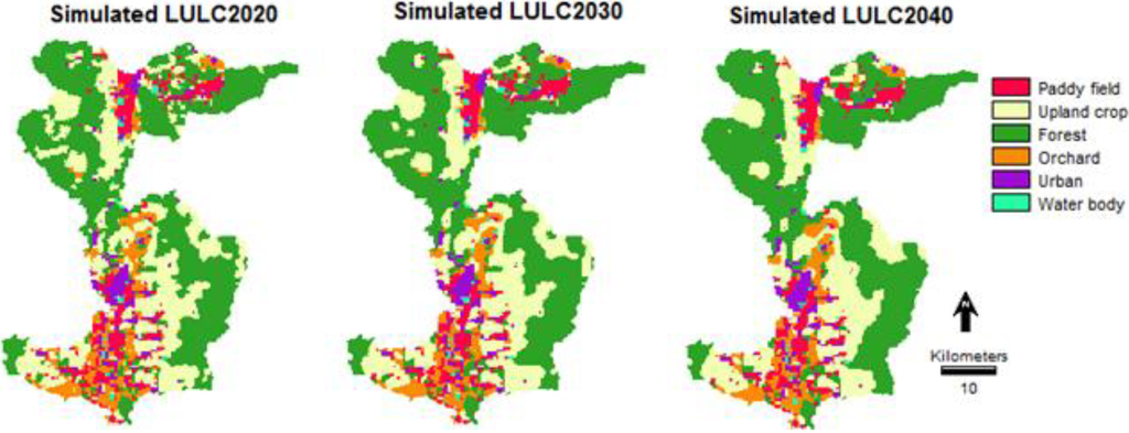
Figure 7.
Simulated LULC maps for the years 2020, 2030 and 2040.
4.3. Rainfall Erosivity (R factor) under Future Climate
Table 9 shows the modified Fournier Index (MFI) versus monthly rainfall and MFI versus rainfall erosivity (R factor) values of each station around the Mea Nam Nan sub-catchment. The MFI values of each station as well as the mathematical formula that relates the MFI value and R factor values have been developed. These mathematical models, which were developed based on historical rainfall data, are ready for use to estimate rainfall erosivity values of each station based on available monthly rainfall data. A power function gives the highest coefficient of determination when compared with seven station simple regression analysis of the monthly rainfall versus the MFI and the R factor versus the MFI. The regression equation has a 0.99 and 0.92 coefficient of statistical determination for data from all stations around the catchment (Figure 8). Figure 9 illustrates the validation between measured and estimated monthly rainfall erosivity (R factor) in the study area and the coefficient determinant (R2), which reflects strength of correlation between the Rmeasured and Rpredicted values of 0.87; this model indicates a good correlation between the variables.
The modified Fournier Index (MFI) values were calculated based on the historical precipitation data and precipitation output from GCM/RCM outputs. Rainfall erosivity is not provided by the current GCM/RCM outputs. The relationship between MFI and the R factor can be used to estimate the monthly and annual rainfall erosivity (R factor) values [12,22]. Therefore, the purpose of this process was to estimate rainfall erosivity under future climate based on GCM/RCM outputs, which consist of HadCM3 and PRECIS RCM under A2 and B2 scenarios and NCAR CCSM3 under A2, A1b and B1. Raw GCM output has been used in many previous studies [9,12,13] of soil erosion under future climate change to disturb erosion models in order to represent future conditions.
Table 9.
The developed modified Fournier index (MFI) and rainfall erosivity (R) predictive model based on observed rainfall.
| Weather station | MFI | R-factor (MJ.mm.ha−1.h−1) | Weather station | MFI | R-factor (MJ.mm.ha−1.h−1) |
|---|---|---|---|---|---|
| Thung Chang | MFI = 0.0006Pm1.98 r² = 0.98 | R = 111MFI0.69 r² = 0.93 | Maung Nan | MFI = 0.0008Pm1.99 r² = 0.99 | R = 78MFI0.71 r² = 0.91 |
| Pou | MFI = 0.0008Pm1.98 r² = 0.99 | R = 96MFI0.70 r² = 0.94 | Viang Sa | MFI = 0.0009Pm1.97 r² = 0.98 | R = 74MFI0.70 r² = 0.93 |
| Tavang pa | MFI = 0.0007Pm1.99 r² = 0.98 | R = 87MFI0.70 r² = 0.91 | Na Noi | MFI = 0.0009Pm1.98 r² = 0.98 | R = 77MFI0.69 r² = 0.92 |
| Agriculture | MFI = 0.0008Pm1.98 r² = 0.99 | R = 81MFI0.71 r² = 0.93 | Average | MFI = 0.0009Pm1.96 r² = 0.99 | R = 85MFI0.71 r² = 0.92 |
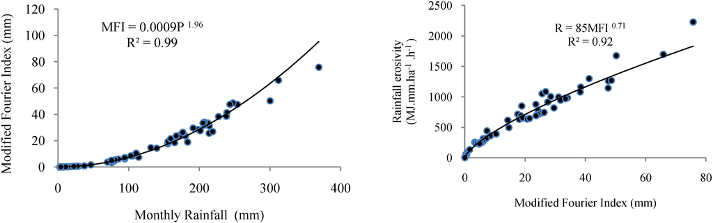
Figure 8.
Relation between MFI and monthly rainfall, rainfall erosivity (R factor) and MFI based on obsereved data.
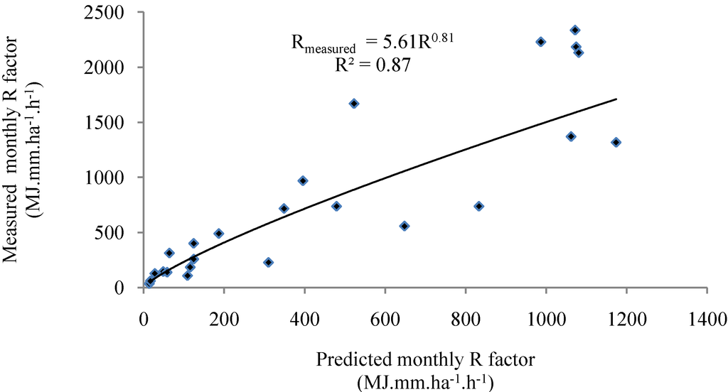
Figure 9.
Scatter plot between measurement and predicted R factor at the validation station.
The Figure 10a–c presents the average monthly precipitation cycle for all climate projections in the three periods and baseline period between 1981 and 2000. Generally, there was a dramatic rise in the precipitation from January until a peak in August was reached. After this, precipitation fell significantly until December. It is clear that there is less monthly average precipitation from PRECIS CCSM3 under A2 and B2 scenarios output than in the base period and other GCMs from March to May, whereas it is equal in comparison with the baseline period from September to December. The precipitation peak range in August of all climate projections is 198–238 mm in 2016–2025, 188–237 mm in 2026–2035 and 196–242 mm in 2036–2045. For annual precipitation the changes range from (Table 11) −13%–9% in 2016–2025, −16%–10% in 2026–2035 and −10%–14% in 2036–2045 depending on the emission scenarios and climate models.
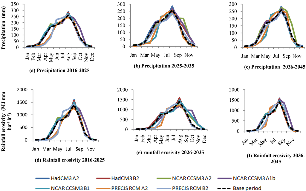
Figure 10.
Average monthly precipitation (a–c) and rainfall erosivity (d–f) for all climate projections for the 2016–2025, 2026–2035, 2035–2046 periods and baseline period 1981–2000 for the Mae Nam Nan sub-catchment.
Unlike precipitation, the changes in monthly rainfall erosivity are not unidirectional for all emission scenarios, climate models and time periods. The intra-annual patterns of rainfall erosivity change from the unimodal. For example, there was a decrease in rainfall erosivity from November to February and an increase in the periods from March to October for all three time periods. Future change of rainfall erosivity (Table 11) in comparison with a base period (5999 MJ mm ha−1 h−1) was between −12%–12% in 2016–2025, −15%–11% in 2026–2035 and −5%–19% in 2036–2045 depending on the emission scenarios and climate models.
4.4. Validation of the RUSLE
For validation of the RUSLE, it is significant to know the measured soil loss in the experimental plots. Figure 11a shows the validation of RUSLE in the study area with R2 = 0.85 which indicates a good amount of balance between measured and estimated soil loss. The mean difference values between the actual and predicted soil loss, or average error (AE) value, was 0.02 t ha−1. Relative error (RE) and standard error (SE) values were 4.20% and 0.38 t ha−1 respectively. The results indicate that the RUSLE model simulates the soil loss in the Mea Nam Nan sub-catchment with reasonable accuracy. Figure 11b illustrates that the variation of measured and estimated soil loss in the experimental plots that predict soil loss is not able to capture peak soil loss events. A soil loss model can be affected by an uncertainty due to the underestimation of soil loss. RUSLE is developed to predict soil loss from agricultural areas. Likewise, the LS factor derived from the digital elevation model (DEM) may not be accurate due to inaccuracies in DEM [69]. In addition, the studied area is located in a tropical climate zone with extreme rainfall and heavy rainstorms which has more potential to erode surface soil [67].
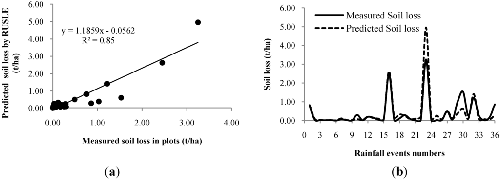
Figure 11.
(a) Validation of Revised Universal Soil Loss Equation (RUSLE) in the study area. (b) Variation of measured and estimated soil loss in the experimental plots.
4.5. Impacts of Climate Change on Soil Loss and Net Soil Loss
Table 10 shows the impact of climate change (precipitation) on future net soil loss at the Mae Nam Nan Sub-catchment. Output from two GCMs (HadCM3 andCCSM3) and a RCM under four emission scenarios (A2, A1b, A2 and B1) were used to downscale precipitation in order to represent changed climatic conditions for soil loss modeling. Use of multiple GCMs and emission scenarios helps to address uncertainties inherent to climate models [44]. The average of the three ensembles reveals that soil erosion decreases from a baseline rate of 0.160 Mg/ha by −4% (0.153 Mg ha−1 y−1) for the period between 2016–2025 and 2036–2045 and by −6 (0.151 Mg ha−1 y−1) for the 2026–2035 period. In addition a decrease in the net soil loss from a baseline of 24,037 Mg y−1 was found to be −4% (23,075 Mg y−1) for the period of 2026–2035 and −5% (22,835 Mg y−1) for the period of 2016–2025. The magnitude of soil erosion change varies depending on the GCM (HadCM3, NCAR CCSM3 and PRECIS RCM) and emission scenario (A2, A1b, A2 and B1). Precipitation decreases and increases of −14% (1078 mm) in the NCAR CCSM3-B1 scenario for the period of 2026–2035s and 16% (1450 mm) in NCAR CCSM3-A2 for the period of 2036–2045 illustrate the predominant factor responsible for increasing and reducing soil erosion rates and net soil loss. Critically, however, it is the timing of precipitation and the amount of daily precipitation intensity rather than merely the average annual precipitation amount that generally controls the response of erosion to climate change.
Table 10.
Change in average annual precipitation net soil loss and net soil loss rate estimated by the sedimentation model for all climate projections under climate change compared to the base period (1981–2000).
| Climate models | Precipitation (mm) | Change (%) | Total erosion (Mg y−1) | Total deposition (Mg y−1) | Net soil loss (Mg y−1) | Change (%) | Net Soil loss rate (Mg ha−1 y−1) | Change (%) |
|---|---|---|---|---|---|---|---|---|
| Base line | 1250 | 40,547 | 16,510 | 24,037 | 0 | 0.160 | 0 | |
| 2016–2025 | ||||||||
| HadCM3-A2 | 1277 | 2 | 44,873 | 17,689 | 27,184 | 13 | 0.180 | 13 |
| HadCM3-B2 | 1275 | 2 | 42,945 | 17,172 | 25,774 | 7 | 0.170 | 6 |
| NCAR CCSM3-A2 | 1282 | 3 | 38,993 | 15,443 | 23,551 | −2 | 0.160 | 0 |
| NCAR CCSM3-A1B | 1369 | 10 | 40,753 | 16,042 | 24,711 | 3 | 0.160 | 0 |
| NCAR CCSM3-B1 | 1327 | 6 | 42,191 | 16,617 | 25,574 | 6 | 0.170 | 6 |
| PRECIS RCM-A2 | 1109 | −11 | 23,543 | 9052 | 14,492 | −40 | 0.100 | −38 |
| PRECIS RCM-B2 | 1113 | −11 | 31,364 | 12,372 | 18,992 | −21 | 0.130 | −19 |
| Average | 1250 | 0 | 37,809 | 14,912 | 22,897 | −5 | 0.153 | −4 |
| 2026–2035 | ||||||||
| HadCM3-A2 | 1279 | 2 | 42,574 | 17,819 | 24,755 | 3 | 0.160 | 0 |
| HadCM3-B2 | 1327 | 6 | 42,438 | 16,866 | 25,572 | 6 | 0.170 | 6 |
| NCAR CCSM3-A2 | 1372 | 10 | 37,426 | 15,255 | 22,171 | −8 | 0.160 | 0 |
| NCAR CCSM3-A1B | 1386 | 11 | 39,829 | 15,747 | 24,083 | 0 | 0.150 | −6 |
| NCAR CCSM3-B1 | 1078 | −14 | 41,856 | 16,254 | 25,602 | 7 | 0.170 | 6 |
| PRECIS RCM-A2 | 1131 | −10 | 31,483 | 12,787 | 18,696 | −22 | 0.120 | −25 |
| PRECIS RCM-B2 | 1164 | −7 | 33,760 | 13,694 | 20,065 | −17 | 0.130 | −19 |
| Average | 1248 | 0 | 38,481 | 15,489 | 22,992 | −4 | 0.151 | −6 |
| 2036–2045 | ||||||||
| HadCM3-A2 | 1275 | 2 | 41,517 | 16,488 | 25,029 | 4 | 0.170 | 6 |
| HadCM3-B2 | 1285 | 3 | 44,837 | 17,507 | 27,330 | 14 | 0.180 | 13 |
| NCAR CCSM3-A2 | 1450 | 16 | 42,292 | 16,349 | 25,944 | 8 | 0.170 | 6 |
| NCAR CCSM3-A1B | 1278 | 2 | 39,415 | 15,503 | 23,911 | −1 | 0.160 | 0 |
| NCAR CCSM3-B1 | 1140 | −9 | 39,198 | 15,646 | 23,552 | −2 | 0.160 | 0 |
| PRECIS RCM-A2 | 1197 | −4 | 28,539 | 11,886 | 16,653 | −31 | 0.110 | −31 |
| PRECIS RCM-B2 | 1165 | −7 | 30,919 | 12,468 | 18,451 | −23 | 0.120 | −25 |
| Average | 1256 | 0 | 38,102 | 15,121 | 22,981 | −4 | 0.153 | −4 |
The soil loss and mean soil loss (Figure 12a) were determined by RUSLE to be between 0–340 Mg ha−1 yr−1 (mean 37 Mg ha−1 yr−1) for 2016–2025, 0–423 Mg ha−1 yr−1 (mean 42 Mg ha−1 yr−1) for 2026–2035 and range of soil loss of 0–414 Mg ha−1 yr−1 (mean 39 Mg ha−1 yr−1) for 2036–2045 under climate change (average rainfall erosivity from HadCM3, NCAR CCSM3, and PRECIS RCM). The net soil loss (erosion and deposition) values estimated by the sedimentation model for 2016–2025, 2026–2035 and 2036–2045 under climate change (Figure 12b) were reclassified into seven classes based on degree of severity [68]. The deposition and erosion risk areas of the different climate change (precipitation) are shown in Figure 13 which illustrates that the percentage of area under erosion risk is stable for the average three future time periods, 55% (83,727 ha) for the period of 2026–2035 and 58% (88,904) for the period of 2016–2025, and that there is a high erosion of 2% (37,766 ha) for the period of 2026–2035 and 3% (4037) for the period of 2036–2045.
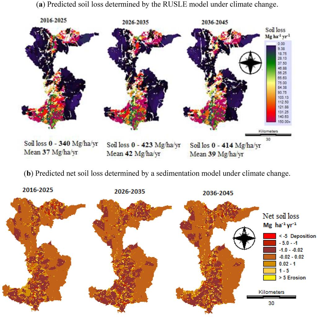
Figure 12.
Maps of soil loss and net soil loss under climate change (Average rainfall erosivity from HadCM3, NCAR CCSM3, and PRECIS RCM).
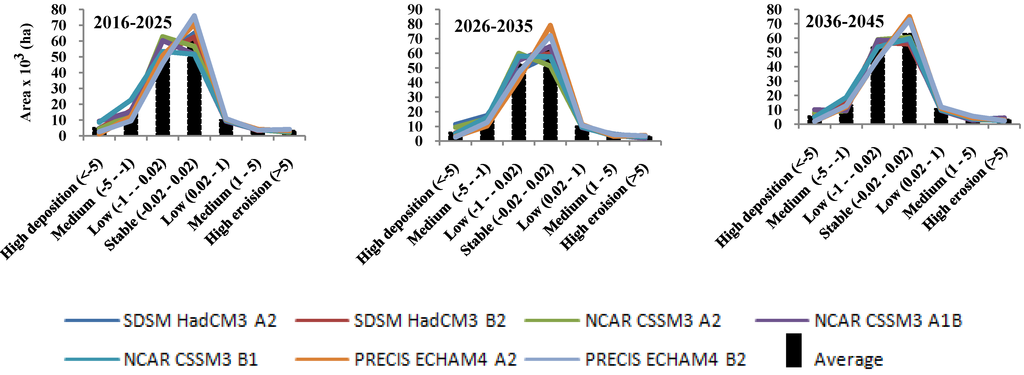
Figure 13.
Average monthly erosion and deposition risk areas for all climate projections and for three future time periods.
Table 11 shows that there is an increase in the area of stable class (−0.02 to 0.02 Mg ha−1 y−1) from the base period, and then the number of areas decreases moderately from 2016–2015 to 2036–2045. The annual net soil loss increases from the baseline amount of 240,37 Mg y−1 by 32% (317,28 Mg y−1) for the period of 2026–2035 and by 44% (34,613 Mg y−1) for the period of 2016–2025. Similarly, annual rates of soil loss for all three future time slices, ranging from increases from the baseline rates of 0.16 Mg ha−1 y−1 by 31% (0.21 Mg ha−1 y−1) for the periods of 2026–2035 and 2036–2045 and by 44% (0.23 Mg ha−1 y−1) for the period of 2016–2025.
Table 11.
Predicted erosion and deposition risk areas and net soil loss under climate change projections from a combination of HadCM3, CCSM3 and PRECIS RCM with A2, A1b, B2 and B1 emissions scenarios for three future time periods.
| Classification | Base line | 2016–2025 | 2026–2035 | 2036–2045 | ||||
|---|---|---|---|---|---|---|---|---|
| Mg ha−1 y−1 | Area (ha) | Soil loss (Mg y−1) | Area (ha) | Soil loss (Mg y−1) | Area (ha) | Soil loss (Mg y−1) | Area (ha) | Soil loss (Mg y−1) |
| High deposition (<−5) | 255 | −3080 | 483 | −5016 | 566 | −6102 | 614 | −6681 |
| Medium (−5–−1) | 1795 | −3269 | 4754 | −8752 | 4136 | −7418 | 5045 | −10,228 |
| Low (−1–−0.02) | 68,459 | −10,059 | 40,284 | −12,209 | 46,254 | −13,163 | 42,250 | −12,747 |
| Stable (−0.02–0.02) | 72,284 | −101 | 88,904 | 10 | 83,727 | −15 | 85,797 | −9 |
| Low (0.02–1) | 5320 | 1436 | 10,541 | 2461 | 11,048 | 2417 | 10,725 | 2219 |
| Medium (1–5) | 2445 | 6580 | 4339 | 10,985 | 3777 | 10,092 | 4806 | 11,939 |
| High erosion (>5) | 2716 | 32,520 | 3969 | 47,071 | 3766 | 45,843 | 4037 | 47,810 |
| Net soil loss (Mg y−1) | 24,037 | 34,548 | 31,654 | 32,304 | ||||
| Change (%) | 0 | 44 | 32 | 34 | ||||
| Rate annual soil loss (Mg ha−1 y−1) | 0.16 | 0.23 | 0.21 | 0.21 | ||||
| Change (%) | 0 | 44 | 31 | 31 | ||||
4.6. Impacts of Land Use Change on Soil Loss and Net Soil Loss
Future soil erosion and deposition at Mae Nam Nan sub-catchment under a changed land use are displayed in Table 12. Figure 14 illustrates the percentage of LULC that has changed between the base period and future land use. Three major increases in the LULC from the base period are found in water bodies in urban areas, and paddy fields amounting to 44%, 76% and 96%, respectively, in three periods. On the other hand, there is a decrease in the percent of LULC change from −37% in 2020 to −47% in 2040. Thus, these LULC have a major effect on soil loss under future land use. Figure 15a shows the impacts of land use change on soil loss to predict by RUSLE. Figure 15a shows the mean soil loss between 157 Mg ha−1 yr−1 in 2020 and 195 Mg ha−1 yr−1 in 2030 under future land use.
Table 12.
Predicted erosion and deposition risk areas and net soil loss under land use change in 2020, 2030 and 2040.
| Classification | Base line | LULC 2020 | LULC 2030 | LULC 2040 | ||||
|---|---|---|---|---|---|---|---|---|
| Mg ha−1 y−1 | Area (ha) | Soil loss (Mg y−1) | Area (ha) | Soil loss (Mg y−1) | Area (ha) | Soil loss (Mg y−1) | Area (ha) | Soil loss (Mg y−1) |
| High deposition (<−5) | 255 | −3080 | 167 | −1186 | 95 | −1010 | 171 | −1936 |
| Medium (−5–−1) | 1795 | −3269 | 1249 | −2306 | 1718 | −2756 | 2291 | −3647 |
| Low (−1–−0.02) | 68,459 | −10,059 | 48,088 | −8228 | 53,239 | −10,942 | 65,973 | −14,226 |
| Stable (−0.02–0.02) | 72,284 | −101 | 94,054 | −168 | 86,127 | −193 | 70,489 | −104 |
| Low (0.02–1) | 5320 | 1436 | 4824 | 1330 | 6264 | 1784 | 7278 | 2609 |
| Medium (1–5) | 2445 | 6580 | 4236 | 8802 | 4749 | 9346 | 5679 | 12,151 |
| High erosion (>5) | 2716 | 32,520 | 656 | 6395 | 1082 | 9960 | 1392 | 12,885 |
| Net soil loss (Mg y−1) | 24,037 | 4639 | 6189 | 7733 | ||||
| Change (%) | 0 | −81 | −74 | −68 | ||||
| Rate annual soil loss (Mg ha−1 y−1) | 0.16 | 0.03 | 0.04 | 0.05 | ||||
| Change (%) | 0 | −81 | −75 | −69 | ||||
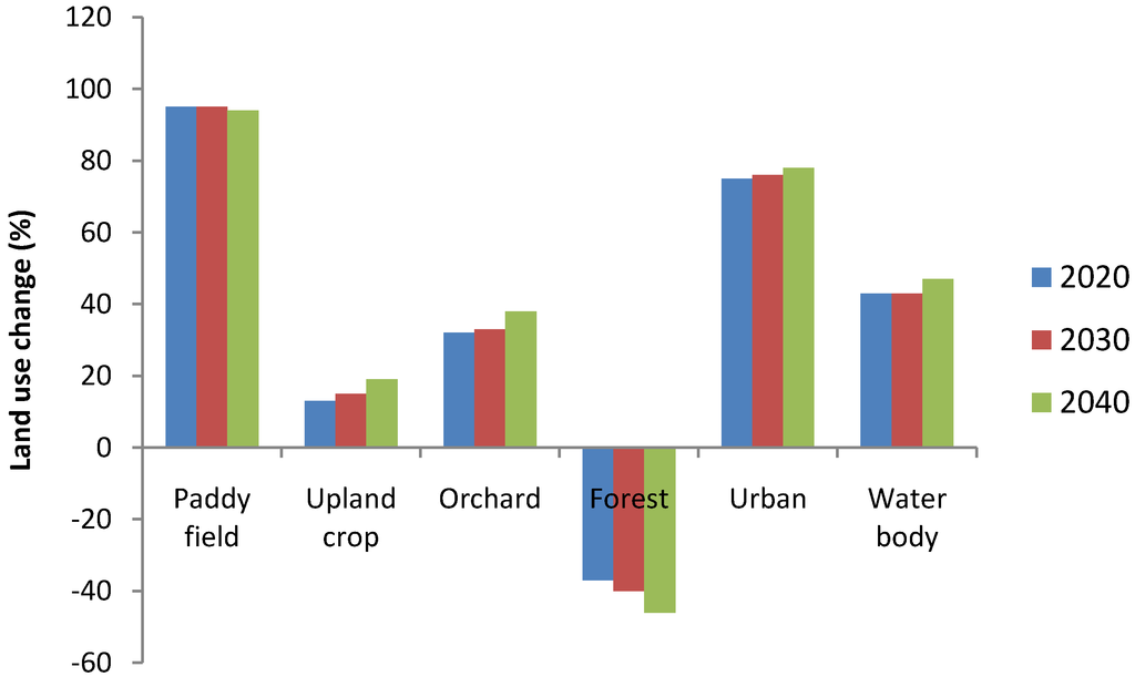
Figure 14.
Land use change between the base period and 2020, 2030 and 2040.
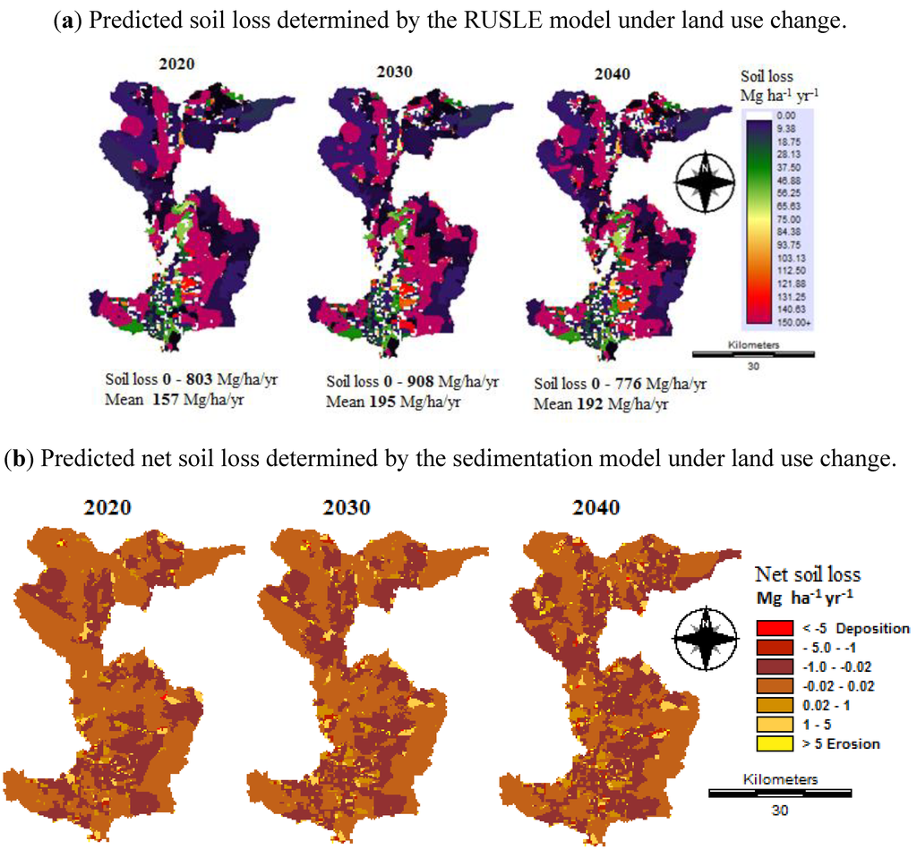
Figure 15.
Maps of soil loss and net soil loss under land use change.
Table 12 shows that the present base period net soil loss is 24,037 Mg y−1, and that the rate of soil loss is 0.16 Mg ha−1 y−1. There is a decrease in net soil loss for all three LULC time periods, from −68% for the LULC 2040 to −81 for the LULC 2020, and an annual soil loss rate from −69% for the LULC 2040 to −81% for the LULC 2020. These decreases reflect the protection provided to the soil by urban and water body areas. Generally, erosion rates dominate the deposition rate for all periods. For intra-deposition and erosion risk areas over 47% (72,284 ha) of the catchment area is stable in the base period, but there is an increase of from 56% (86,127 ha) in 2030 to 61% (94,054 ha) in 2020 in the catchment area in the stable class in the future. It is noticeable that a high stable area is located in the forest area (Figure 15b).
4.7. Impacts of Land Use and Climate Change on Soil Loss and Net Soil Loss (Full Range of Impacts)
Table 13 shows the response of net soil erosion at the Mae Nam Nan sub-catchment under climate and land use change (full range of impacts). Drastic decreases in soil loss rate and net soil erosion are evident under all scenarios, with soil erosion decreasing from the baseline rate of 0.16 Mg ha−1 y−1 to the lowest decrease of 0.06 Mg ha−1 y−1 under the NCAR CCSM3-A1B and B1 scenarios for the 2036–2045 period and up to the highest increase of 0.02 Mg ha−1 y−1 under the PRECIS RCM-A2 scenario for the 2016–2025 period. Similarly, there was a decrease in net soil loss from the base line of 24,037 Mg y−1 of between 8412 Mg y−1 under NCAR CCSM3-B1 (2036–2045) and 3125 Mg y−1 under PRECIS RCM-A2 for the (2016–2025).
Table 13.
Changes in average annual rainfall erosivity, net soil loss estimated by the sedimentation model under full range of impact (climate and land use change) compared to the base period.
| Climate models | Rainfall erosivity (MJ mm ha−1 h−1) | Change (%) | Total erosion (Mg/y) | Total deposition (Mg/y) | Net soil loss (Mg/y) | Change (%) | Net Soil loss rate (Mg /ha) | Change (%) |
|---|---|---|---|---|---|---|---|---|
| Base line | 5999 | 0 | 40,547 | 16,510 | 24,037 | 0 | 0.16 | 0 |
| 2016–2025 | ||||||||
| HadCM3-A2 | 5808 | −3 | 16,287 | 12,017 | 4270 | −82 | 0.03 | −81 |
| HadCM3-B2 | 5800 | −3 | 15,589 | 11,381 | 4208 | −82 | 0.03 | −81 |
| NCAR CCSM3-A2 | 5868 | −2 | 17,405 | 12,649 | 4756 | −80 | 0.03 | −81 |
| NCAR CCSM3-A1B | 6384 | 6 | 17,258 | 12,678 | 4580 | −81 | 0.03 | −81 |
| NCAR CCSM3-B1 | 6144 | 2 | 17,106 | 12,368 | 4738 | −80 | 0.03 | −81 |
| PRECIS RCM-A2 | 5015 | −16 | 11,025 | 7986 | 3039 | −87 | 0.02 | −88 |
| PRECIS RCM-B2 | 5244 | −13 | 15,432 | 10,679 | 4753 | −80 | 0.03 | −81 |
| Average | 5752 | −4 | 15,729 | 11,394 | 4335 | −82 | 0.03 | −81 |
| 2026–2035 | ||||||||
| HadCM3-A2 | 5838 | −3 | 20,620 | 14,165 | 6455 | −73 | 0.04 | −75 |
| HadCM3-B2 | 5822 | −3 | 21,203 | 15,272 | 5931 | −75 | 0.04 | −75 |
| NCAR CCSM3-A2 | 5917 | −1 | 22,693 | 16,226 | 6467 | −73 | 0.05 | −69 |
| NCAR CCSM3-A1B | 6152 | 3 | 22,598 | 16,218 | 6380 | −73 | 0.04 | −75 |
| NCAR CCSM3-B1 | 6322 | 5 | 21,715 | 15,538 | 6177 | −74 | 0.04 | −75 |
| PRECIS RCM-A2 | 4866 | −19 | 19,476 | 13,472 | 6004 | −75 | 0.04 | −75 |
| PRECIS RCM-B2 | 5231 | −13 | 20,039 | 13,944 | 6095 | −75 | 0.04 | −75 |
| Average | 5735 | −4 | 21,192 | 14,976 | 6216 | −74 | 0.04 | −75 |
| 2036–2045 | ||||||||
| HadCM3-A2 | 5820 | −3 | 29,010 | 21,657 | 7353 | −69 | 0.05 | −69 |
| HadCM3-B2 | 5784 | −4 | 27,809 | 20,326 | 7483 | −69 | 0.05 | −69 |
| NCAR CCSM3-A2 | 5915 | −1 | 28,785 | 21,099 | 7686 | −68 | 0.05 | −69 |
| NCAR CCSM3-A1B | 6917 | 15 | 29,801 | 21,865 | 7936 | −67 | 0.06 | −63 |
| NCAR CCSM3-B1 | 5897 | −2 | 31,321 | 22,949 | 8372 | −65 | 0.06 | −63 |
| PRECIS RCM-A2 | 5321 | −11 | 22,509 | 16,512 | 5997 | −75 | 0.04 | −75 |
| PRECIS RCM-B2 | 5646 | −6 | 24,745 | 18,304 | 6441 | −73 | 0.04 | −75 |
| Average | 5900 | −2 | 27,711 | 20,387 | 7324 | −70 | 0.05 | −69 |
It is noticeable that the significant decrease in soil loss rates and net soil erosion reflects a combination of all the factors discussed with respect to the aforementioned scenarios. The key factor is the land-use change since there was an increase in urban and water body areas, which are affected by crop and management factors. The highest decrease in soil loss under the full range of impacts occurs because of change in land use. Figure 16a illustrates the spatial distribution patterns of the different soil losses. It was estimated by RUSLE for impacts of land use and climate change (full range of impact) based on future land use and combinations of two general circulation models (HadCM3 and NCAR CCSM3) and a regional climate model (PRECIS RCM). There was an increase in mean soil loss from 114 Mg ha−1 y−1 for 2016–2025) to 130 Mg ha−1 y−1 for the period of 2036–2045.
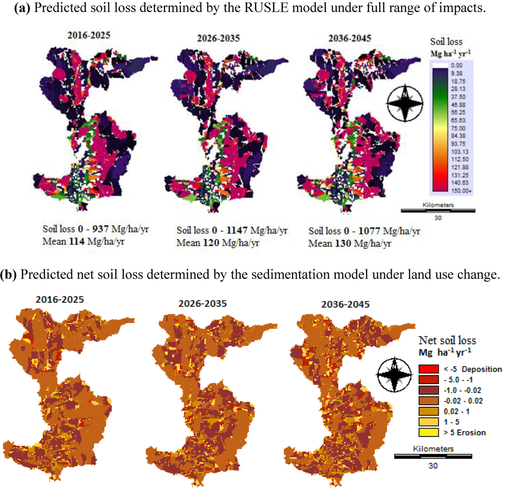
Figure 16.
Maps of soil loss and net soil loss under land use and climate change (full range of impacts).
Figure 16b illustrates the spatial distribution of net soil loss risk (erosion and deposition) estimated by the sedimentation model under the impacts of land use and climate change projections from a combination of HadCM3, CCSM3 and PRECIS RCM with A2, A1b, B2 and B1 emission scenarios for three future time periods. The dramatic decreases in erosion rates and net soil loss reflect a combination of all the factors. Table 14 shows future erosion rates, which are displayed as total and percentage changes with GCM/RCM emission scenario combinations. There was a dramatic decrease in net soil loss from the baseline of 240,37 Mg y−1 of between 17,306 Mg y−1 for 2036–2045 and 11,778 Mg y−1 for 2016–2025. Similarly, the rate of soil loss decreased significantly from the base line of 0.16 Mg/ha, ranging from 0.08 Mg ha−1 y−1 for 2016–2025 to 0.12 Mg ha−1 y−1 for 2036–2045. Therefore, the full ranges of impacts have two factors, which consist of LULC conversion towards decreased tillage (indirect impact) and the increased precipitation (direct impact), the combined result of which is a large decrease in soil erosion at the Mea Nam Nan sub-catchment.
Table 14.
Predicted soil loss rates and soil erosion/deposition risk areas under climate and land use change projections (full range of impacts) from a combination of HadCM3, CCSM3 and PRECIS RCM with A2, A1b, B2 and B1 emission scenarios for three future time periods.
| Classification | Base line | 2016-2025 | 2026-2035 | 2036-2045 | ||||
|---|---|---|---|---|---|---|---|---|
| Mg ha−1 y−1 | Area (ha) | Soil loss (Mg y−1) | Area (ha) | Soil loss (Mg y−1) | Area (ha) | Soil loss (Mg y−1) | Area (ha) | Soil loss (Mg y−1) |
| High deposition (<−5) | 255 | −3080 | 598 | −4958 | 750 | −7598 | 610 | −6964 |
| Medium (−5–−1) | 1795 | −3269 | 4850 | −8975 | 4706 | −9454 | 8566 | −15,969 |
| Low (−1–−0.02) | 68,459 | −10,059 | 42,637 | −11,971 | 51,000 | −14,815 | 48,084 | −13,622 |
| Stable (−0.02–0.02) | 72,284 | −101 | 86,848 | −46 | 76,494 | −32 | 72,385 | −21 |
| Low (0.02–1) | 5320 | 1436 | 10,281 | 3347 | 11,047 | 3236 | 12,132 | 3968 |
| Medium (1–5) | 2445 | 6580 | 5962 | 12,966 | 6836 | 17,020 | 8606 | 21,026 |
| High erosion (>5) | 2716 | 32,520 | 2098 | 21,439 | 2441 | 25,437 | 2891 | 28,824 |
| Net soil loss (Mg y−1) | 24,037 | 11,802 | 13,794 | 17,242 | ||||
| Change (%) | 0 | −51 | −43 | −28 | ||||
| Rate annual soil loss (Mg ha−1 y−1) | 0.16 | 0.08 | 0.1 | 0.12 | ||||
| Change (%) | 0 | −50 | −38 | −25 | ||||
5. Discussion
The impacts of climate change on soil loss and net soil loss (erosion and deposition) may increase or decrease at the Mae Nam Nan sub-catchment depending on the interacting effects of the factors considered. It can be seen that the mean soil loss determined by the RUSLE model (Figure 12a) under climate change projections from a combination of HadCM3, CCSM3 and PRECIS RCM with A2, A1b, B2 and B1 emission scenarios for three future time slices are between 37 Mg ha−1 y−1 for 2016–2025 and 42 Mg ha−1 y−1 for 2026–2035. Table 11 shows that there is a increase in net soil loss estimated by sedimentation model, ranging in increases from the base line of 24,037 Mg y−1 of between 31,654 Mg y−1 for 2026–2035 and 34,548 Mg y−1 for 2016–2025. If downscaled climate change projections are considered in isolation, then future rates of soil erosion and deposition are generally projected to rise due to increases in precipitation and rainfall erosivity in the future. This is in accordance with similar studies [7,8,10,12] on soil erosion, which suggest that increased precipitation amounts and intensities will lead to greater rates of erosion. The expected increase in precipitation may have significant effects on soil loss.
The mean soil loss was determined by the RUSLE model under a land use change between 157 Mg ha−1 y−1 in 2020 and 195 Mg ha−1 y−1 in 2030 (Figure 15a–b). Similarly, net soil losses estimated by the sedimentation model for all three future time periods decrease dramatically from a base line of 24,037 Mg y−1 to 4,639 Mg y−1 for 2020 and 7,733 Mg y−1 for 2040. Land use is the most crucial element in the soil erosion model. Land use change factors are practically the most difficult to predict with confidence. Soil loss and net soil loss potential maps were generated based on the past (1990) and future land use (2020, 2030 and 2040) and other spatially derived parameters using the RUSLE and sedimentation models. When land use change and management are added to the modeling process, however, then soil loss rate, soil erosion and deposition are projected to decrease significantly from the baseline period, depending on the specific land use scenarios. Areas of high erosion can be rapidly identified, and management efforts can be directed at these high priority areas. In this study, high erosion and deposition zones indentified areas along the Nan River. Thus, improved vegetation conditions such as vetiveria grass should be recommended to the farmers in order to reduce soil loss in slope areas. For example, it should be recommended to plant vetiveria grass against the slope and along the riverside to capture sedimentation and to grow it on check-dams, which helps to protect against soil erosion.
It can be seen that there was a decrease in net soil loss estimated by sedimentation (Table 14) under climate change projections from a combination of HadCM3, CCSM3 and PRECIS RCM with A2, A1b, B2 and B1 emission scenarios for three future time periods from a baseline of 24,037 Mg y−1 of between 11,802 Mg y−1 for 2020 and 17,733 Mg y−1 for 2040. When an additional R factor (climate change) and C factor (land use change) are included in the modeling process, soil erosion rates and net soil loss are projected to decrease dramatically. However, the increase in rainfall can be expected through the increase in the number of rain days and the increase in rainfall intensity. The study conducted by Pruski and Nearing [13] indicates that changes in rainfall that occur due to changes in storm intensity can be expected to have a greater impact on erosion rates than those due to changes in the number of rain days alone. Further studies are necessary to consider the impact of rainfall intensity on potential changes in rainfall erosivity and soil erosion and deposition in the Mea Nam Nan sub-catchment.
6. Limitations of This Study
There are several limitations in this paper. A major one is that uncertainties of a range of possible climate change consist of uncertainty surrounding future climate change projections (emissions and GCMs/RCMs) and downscaling methods. The downscaling method (delta change method) also creates uncertainties in downscaled climate data sets in part because GCMs are optimized to forecast climate change at their native resolutions [70]. The delta change method is a simple way to implement and acquire information from just a GCMs/RCM monthly time scale. On the other hand, many statistical downscaling methods need data from just GCMs on a daily time scale. Daily scale data from GCMs are considered less accurate by many [71,72]. Also, bias correction and variance adjustment is often needed to obtain adequate results, whereas with the change factor method, bias correction is implicitly built into the approach [59]. Another limitation of this study is that the CA_Markov mode was the time duration used for the LULC change prediction, although it should be the same time period for the database used in the study. However, this paper studies land use change in the year 2010 derived from the CA_Markov model compared with the results from LULC classification in 2010 by the segmentation classification. Hence the result from the prediction is different from the time duration for the LULC prediction in the years 2020, 2030 and 2040 estimated by the CA_Markov mode (for which the time duration change was 20, 30 and 40 years) and was derived from LULC change for the period of 10 years (from 1990 to 2000).
7. Conclusions
This study simulates the impacts of climate change, land use change and their combined effects on soil loss and net soil loss in the Mae Nam Nan sub-catchment, Thailand. In this study, a multi-climate model and a multi-emission scenario approach for the estimation of climate change impacts are used. The delta change method is used as a downscaling technique to generate future precipitation. The soil loss model using Revised Universal Soil Loss Equation (RUSLE) and sedimentation model in Idrisi software are used to simulate the present and future changes in soil erosion and deposition in the study area. Results indicate that soil erosion and deposition changes are not unidirectional and vary depending on the greenhouse gas emission scenarios and land use scenarios. The potential for climate change to increase soil loss rate, soil erosion and deposition in future periods are established, whereas considerable decreases in soil erosion and deposition are projected when land use is increased (paddy fields, urban areas and water body) from baseline periods. The combined climate and land use change analysis reveals that land use planning can be adopted to mitigate soil erosion and deposition in the future, in conjunction with the projected direct impact of climate change. The results of this study may be helpful to development planners and decision makers when planning and implemented suitable soil erosion control and sediment management plans to adapt to land use and climate change.
Acknowledgements
The authors would like to thank Pornchai Mongkhonvanit for financial assistance. We are also thankful to the PRECIS RCM data from the Southeast Asia START Regional Center [55], the NCAR Community Climate System Model (CCSM) projections in GIS formats [54], Precipitation data from Thai Meteorological Department and the Landsat TM data from US Geological Survey (USGS).
Conflict of Interest
The authors declare no conflict of interest.
References
- Yang, D.; Kanae, S.; Oki, T.; Koike, T.; Musiake, K. Global potential soil erosion with reference to land use and climate changes. Hydrol. Process. 2003, 17, 2913–2928. [Google Scholar] [CrossRef]
- Feng, X.; Wang, Y.; Chen, L.; Fu, B.; Bai, G. Modelling soil erosion and its response to land-use change in hilly catchments of the Chinese Loess Plateau. Geomorphology 2010, 118, 239–248. [Google Scholar] [CrossRef]
- Land Development Department, Soil Erosion in Thailand; (in Thai). Soil and Water Conservation Division, Land Development Department: Bangkok, Thailand, 2002.
- Schertz, D.L.; Moldenhauer, W.C.; Livingston, S.J.; Weesies, G.A.; Hintz, E.A. Effect of past soil erosion on crop productivity in Indiana. J. Soil Water Conserv. 1989, 44, 604–608. [Google Scholar]
- Beniston, M. Mountain weather and climate: A general overview and a focus on climatic change in the Alps. Hydrobiologia 2006, 562, 3–16. [Google Scholar] [CrossRef]
- Zhang, X.C.; Nearing, M.A. Impact of climate change on soil erosion, runoff and wheat productivity in central Oklahoma. Catena 2005, 61, 185–195. [Google Scholar] [CrossRef]
- Michael, A.; Schmidt, J.; Enke, W.; Deutschlander, T.; Maltiz, G. Impact of expected increase in precipitation intensities on soil loss results of comparative model simulations. Catena 2005, 61, 155–164. [Google Scholar] [CrossRef]
- Neal, M.R.; Nearing, M.A.; Vining, R.C.; Southworth, J.; Pfeifer, R.A. Climate change impacts on soil erosion in Midwest United States with changes in crop management. Catena 2005, 61, 165–184. [Google Scholar] [CrossRef]
- Favis-Mortlock, D.T.; Boardman, J. Nonlinear responses of soil erosion to climate change: A modelling study on the UK South Downs. Catena 1995, 25, 365–387. [Google Scholar] [CrossRef]
- Favis-Mortlock, D.T.; Guerra, A.J.T. The implications of general circulation model estimates of rainfall for future erosion: A case study from Brazil. Catena 1999, 37, 329–354. [Google Scholar] [CrossRef]
- Mullan, D.; Favis-Mortlock, D.T.; Fealy, R. Addressing key limitations associated with modelling soil erosion under the impacts of future climate change. Agric. Forest. Meteorol. 2012, 156, 18–30. [Google Scholar] [CrossRef]
- Shrestha, B.; Babel, M.S.; Maskey, S.; Griensven, A.V.; Uhlenbrook, S.; Green, A.; Akkharath, I. Impact of climate change on sediment yield in the Mekong River basin: A case study of the Nam Ou basin, Lao PDR. Hydrol. Earth Syst. Sci. 2013, 17, 1–20. [Google Scholar] [CrossRef]
- Pruski, F.F.; Nearing, M.A. Climate-induced changes in erosion during the 21st century for eight U. S. locations. Water Resour. Res. 2002, 38, 34–44. [Google Scholar]
- Wischmeier, W.H.; Smith, D.D. Predicting Rainfall Erosion Losses. In USDA Agric. Handbook; Agricultural Research Service: Washington, DC, USA, 1978; Volume 537, p. 58. [Google Scholar]
- Renard, K.G.; Foster, G.A.; Weesies, G.A.; McCool, D.K.; Yoder, D.C. Predicting Soil Erosion by Water: A Guide to Conservation Planning with the Revised Universal Soil Loss Equation (RUSLE). In USDA Agriculture Handbook; Agricultural Research Service: Washington, DC, USA, 1997; Volume 703, p. 404. [Google Scholar]
- Clemente, R.S.; Prasher, S.O.; Barrington, S.F. PESTFADE—A new pesticide fate and transport model: Model development and verification. Trans. ASAE. 1993, 36, 357–367. [Google Scholar]
- Sukhanovski, Y.P.; Ollesch, G.; Khan, K.Y.; Meissner, R. A new index for rainfall erosivity on a physical basis. J. Plant Nutr. Soil Sci. 2001, 165, 51–57. [Google Scholar]
- Mannaerts, C.M.; Gabriels, D. Rainfall erosivity in Cape Verde. Soil Till. Res. 2000, 55, 207–212. [Google Scholar] [CrossRef]
- Solomon, S.D.; Qin, M.M.; Chen, M.M.; Marquis, K.B.; Averyt, M.T.; Millers, H.L. (Eds.) IPCC. Summary for policy makers. In Climate Change 2007: The Physical Science Basis; Proceedings of the 10th Working Group I Session, Paris, 29 January–1 February 2007; Cambridge University Press: Cambridge, UK, New York, NY, USA, 2007.
- Nearing, A.M. Potential changes in rainfall erosivity in the U. S. with climate change during the 21st century. J. Soil Water Conserv. 2001, 56, 229–232. [Google Scholar]
- Zhang, X.C. A comparison of explicit and implicit spatial downscaling of GCM output for soil erosion and crop production assessments. Clim. Chang. 2007, 84, 337–363. [Google Scholar] [CrossRef]
- Renard, K.G.; Fremund, J.R. Using monthly precipitation data to estimate the R-factor in the revised USLE. J. Hydrol. 1994, 157, 287–306. [Google Scholar] [CrossRef]
- Komas, C.; Danalatos, N.; Cammeraat, L.H.; Chabart, M.; Diamantopoulos, J.; Farand, R.; Gutierrez, L.; Jacob, A.; Marques, H.; Martinez-Fernandez, J.; et al. The effect of land use on runoff and soil erosion rates under Mediterranean conditions. Catena 1997, 29, 45–59. [Google Scholar] [CrossRef]
- Szilassi, P.; Jordan, G.; van Rompaey, A.; Csillag, G. Impact of historical land use changes on erosion and agricultural soil properties in Kali Basin at Lake Balaton, Hungary. Catena 2006, 68, 96–108. [Google Scholar] [CrossRef]
- Zhou, P.; Luukkanen, O.; Tokola, T.; Nieminen, J. Effect of vegetation cover on soil erosion in a mountainous watershed. Catena 2008, 75, 319–325. [Google Scholar] [CrossRef]
- Solaimani, K.; Modallaldoust, S.; Lotfi, S. Investigation of land use changes on soil erosion process using geographical information system. Int. J. Environ. Sci. Technol. 2009, 6, 415–424. [Google Scholar]
- Su, Z.A.; Zhang, J.H.; Nie, X.J. Effect of soil erosion on soil properties and crop yields on slopes in the Sichuan Basin, China. Pedosphere 2010, 20, 736–746. [Google Scholar] [CrossRef]
- Cotler, H.; Ortega-Larrocea, M.P. Effects of land use on soil erosion in a tropical dry forest ecosystem, Chamela watershed, Mexico. Catena 2006, 65, 107–117. [Google Scholar] [CrossRef]
- Cebecauer, T.; Hofierka, J. The consequences of land-cover changes on soil erosion distribution in Slovakia. Geomorphology 2008, 98, 187–198. [Google Scholar] [CrossRef]
- Mohammad, A.G.; Adam, M.A. The impact of vegetation cover type on runoff and soil erosion under different land uses. Catena 2010, 81, 97–103. [Google Scholar] [CrossRef]
- Gyssels, G.; Poesen, J.; Bochet, E.; Li, Y. Impact of plant roots on the resistance of soils to erosion by water: A review. Prog. in Phys. Geogr. 2005, 29, 189–217. [Google Scholar] [CrossRef]
- Bewket, W.; Teferi, E. Assessment of soil erosion hazard and prioritization for treatment at the watershed level: Case study in the Chemoga watershed, Blue Nile basin, Ethiopia. Land. Degrad. Dev. 2009, 20, 609–622. [Google Scholar] [CrossRef]
- López-Vicente, M.; Navas, A. Routing runoff and soil particles in a distributed model with GIS: Implications for soil protection in mountain agricultural landscapes. Land. Degrad. Dev. 2010, 21, 100–109. [Google Scholar] [CrossRef]
- Mutua, B.M.; Klik, A.; Loiskandl, W. Modelling soil erosion and sediment yield at a catchment scale: The case of Masinga catchment, Kenya. Land. Degrad. Dev. 2006, 17, 557–570. [Google Scholar] [CrossRef]
- Wischmeier, W.H. Use and misuse of the universal soil loss equation. J. Soil Water Conserv. 1976, 31, 5–9. [Google Scholar]
- Land Development Department, Thailand. In Land Use Map of Nan Province; (in Thai). Land Use Planning Division, Land Development Department: Bangkok, Thailand, 2006.
- Moore, I.D.; Burch, G.J. Modelling erosion and deposition: Topographic effects. Trans. ASAE. 1986, 29, 1624–1640. [Google Scholar]
- Fernandez, C.; Wu, J.Q.; McCool, D.K.; Stockle, C.O. Estimating water erosion and sediment yield with GIS, RUSLE, and SEDD. J. Soil Water Conserv. 2003, 58, 128–136. [Google Scholar]
- Lewis, L.A.; Verstraeten, G.; Zhu, H. RUSLE applied in a GIS framework: Calculating the LS factor and deriving homogeneous patches for estimating soil loss. Int. J. Geogr. Inf. Sci. 2005, 19, 809–829. [Google Scholar] [CrossRef]
- Fu, B.J.; Zhao, W.W.; Chen, L.D.; Zhang, Q.J.; Lu, Y.H.; Gulinck, H.; Poesen, J. Assessment of soil erosion at large watershed scale using RUSLE and GIS: A case study in the loess plateau of China. Land. Degrad. Dev. 2005, 16, 73–85. [Google Scholar] [CrossRef]
- Fu, G.; Chen, S.; McCool, D.K. Modeling the impacts of no-till practice on soil erosion and sediment yield with RUSLE, SEDD, and ArcView GIS. Soil Till. Res. 2006, 85, 38–49. [Google Scholar] [CrossRef]
- Nekhay, O.; Arriaza, M.; Boerboom, L. Evaluation of soil erosion risk using analytic network process and GIS: A case study from Spanish mountain olive plantations. J. Environ. Manag. 2009, 90, 3091–3104. [Google Scholar] [CrossRef]
- Capolongo, D.; Pennetta, L.; Piccarreta, M.; Fallacara, G.; Boenzi, F. Spatial and temporal variations in soil erosion and deposition due to land-levelling in a semi-arid area of Basilicata (Southern Italy). Earth Surf. Process. Landf. 2008, 33, 364–379. [Google Scholar] [CrossRef]
- Land Development Department, Group of Soil Series for Economic Crops of Thailand; (in Thai). Soil Survey and Land use Planning Division, Land Development Department: Bangkok, Thailand, 2005.
- Congalton, R.G. A review of assessing the accuracy of classifications of remotely sensed data. Remote Sens. Environ. 1990, 37, 35–46. [Google Scholar] [CrossRef]
- Chen, H.; El Garouani, A.; Lewis, L.A. Modelling soil erosion and deposition within a Mediterranean mountainous environment utilizing remote sensing and SIG- Wadi Tlata. Morocco. Geogr. Helv. 2008, 63, 36–47. [Google Scholar] [CrossRef] [Green Version]
- EI Aroussi, O.; Mesrar, L.; Lakrim, M.; EI Garouani, A.; Jabrane, R. Methodological approach for assessing the potential risk of soil erosion using remote sensing and GIS in the Oued EI Malleh watershed. J. Mater. Environ. Sci. 2011, 2, 433–438. [Google Scholar]
- Wischmeier, W.H.; Smith, D.D. Rainfall energy and its relationship to soil loss. Trans. Am. Geophys. Union. 1958, 39, 285–291. [Google Scholar] [CrossRef]
- Foster, G.R.; McCool, D.K.; Renard, K.G.; Moldenhauer, W.C. Conversion of the universal soil loss equation to SI metric units. J. Soil Water Consev. 1991, 36, 355–359. [Google Scholar]
- Brown, L.C.; Foster, G.R. Strom erosivity using idealized intensity distributions. Trans. Am. Soc. Agric. Eng. 1987, 30, 372–386. [Google Scholar]
- Arnoldus, H.M.J. Methodology used to determine the maximum potential average annual soil loss due to sheet and rill erosion in Morocco. FAO Soil Bull. 1977, 34, 39–51. [Google Scholar]
- Ferro, V.; Porto, P.; Yu, B. A comparative study of rainfall erosivity estimation for southern Italy and southeastern Australia. Hydrol. Sci. J. 1999, 44, 3–24. [Google Scholar] [CrossRef]
- Grazhdani, S.; Shumka, S. An approach to mapping soil erosion by water with application to Albania. Desalination 2007, 213, 263–272. [Google Scholar] [CrossRef]
- Download NCAR Community Climate System Model (CCSM) Projections in GIS formats. Available online: https://gisclimatechange.ucar.edu/gis-data (accessed on 5 January 2013).
- View Regional Climate Change. Available online: http://cc.start.or.th/start2/default.asp (accessed on 5 January 2013).
- Fowler, H.J.; Blenkinsop, S.; Tebald, C. Linking climate change modelling to impacts studies: Recent advances in downscaling techniques for hydrological modeling. Int. J. Climatol. 2007, 27, 1547–1578. [Google Scholar] [CrossRef]
- Hay, L.E.; Wilby, R.L.; Leavesly, H.H. Comparison of delta change and downscaled GCM scenarios for three mountainous basins in the United States. J. Am. Water Resour. Assoc. 2000, 36, 387–397. [Google Scholar] [CrossRef]
- Diaz-Nieto, J.; Wilby, R.L. A comparison of statistical downscaling and climate change factor methods: Impacts on low flows in the river Thames. United Kingdom. Clim. Chang. 2005, 69, 245–268. [Google Scholar] [CrossRef]
- Akhtar, M.; Ahmad, N.; Booij, M.J. The impact of climate change on the water resources of Hindukush-Karakorum-Himalaya region under different glacier coverage scenarios. J. Hydrol. 2008, 355, 148–163. [Google Scholar] [CrossRef]
- Minville, M.; Brissette, F.; Leconte, R. Uncertainty of the impact of climate change on the hydrology of a Nordic watershed. J. Hydrol. 2008, 358, 70–83. [Google Scholar] [CrossRef]
- Chen, J.; Brissette, F.P.; Leconte, R. Uncertainty of downscaling method in quantifying the impact of climate change on hydrology. J. Hydrol. 2011, 401, 190–202. [Google Scholar] [CrossRef]
- Land Development Department, Soil Erosion in Thailand; (in Thai). Soil and Water Conservation Division, Land Development Department: Bangkok, Thailand, 2000.
- Eastman, J.R. Idrisi Taiga Guide to GIS and Image Processing; Clark University: Worcester, MA, USA, 2009. [Google Scholar]
- Thitirojanawat, P. Comparative Study of Soil Loss Estimation by Universal Soil Loss Equation (USLE) and Runoff Plots at Nan Watershed Area, Northern Thailand. Master Thesis, Mahidol University, Thailand, 1993. [Google Scholar]
- Tangtham, N. Mathematical Models of Soil Erosion and Sediment Pollution in Watershed. Department of Conservation, Faculty of Forestry; Kasetsart University: Bangkok, Thailand, 2002. [Google Scholar]
- Rasmussen, S. An Introduction to Statistics with Data Analysis; Brooks/Cole: Pacific Grove, CA, USA, 1992. [Google Scholar]
- Pongsai, S.; Vogt, D.S.; Shrestha, R.P.; Clemente, R.S.; Eiumnoh, A. Calibration and validation of the modified universal soil loss equation for estimating sediment yield on sloping plots: A case study in Khun Satan catchment of northern Thailand. Can. J. Soil Sci. 2010, 90, 585–596. [Google Scholar] [CrossRef]
- Muzein, B.S. Remote sensing and GIS for land cover/land use change detection and analysis in the semi-natural ecosystems and agriculture landscapes of the central Ethiopian Rift Valley. Ph.D. Dissertation, Techniche Universität Dresden, Dresden, Germany, 2006. [Google Scholar]
- Babel, M.S.; Shrestha, B.; Perret, S. Hydrological impact of biofuel production: A case study of the Khlong Phlo Watershed in Thailand. Agric. Water Manag. 2011, 101, 8–26. [Google Scholar] [CrossRef]
- Wilby, R.L.; Charles, S.P.; Zorita, E.; Timbal, B.; Whetton, P.; Mearns, L.O. Guidelines for Use of Climate Scenarios Developed from Statistical Downscaling Methods. IPCC Task Group on Data and Scenario Support for Impact and Climate Analysis (TGICA). Available online: http://ipcc-ddc.cru.uea.ac.uk/guidelines/StatDown_Guide.pdf (accessed on 20 December 2012).
- Huth, R.; Kysely, J.; Dubrovsky, M. Time structure of observed, GCM-simulated, downscaled, and stochastically generator daily temperature series. J. Climate. 2001, 14, 4047–4061. [Google Scholar] [CrossRef]
- Palutikof, J.P.; Winkler, J.A.; Goodess, C.M.; Andresen, J.A. The simulation of daily temperature time series from GCM Output. Part 1: Comparison of model data with observations. J. Climate. 1997, 10, 2497–2513. [Google Scholar] [CrossRef]
© 2013 by the authors; licensee MDPI, Basel, Switzerland. This article is an open access article distributed under the terms and conditions of the Creative Commons Attribution license (http://creativecommons.org/licenses/by/3.0/).