Abstract
City noise is a significant health issue, particularly in expanding metropolitan areas like Charlotte, North Carolina. This research examines the potential for vegetation density to mitigate transportation noise as a sustainable solution. The analysis used the Normalized Difference Vegetation Index (NDVI), population density, and transportation noise zones from the USA Department of Transportation, evaluated at the census block group level all for 2020. To identify overall patterns, a Spatial Autoregressive (SAR) model and Geographically Weighted Regression (GWR) were used for spatial structure and local variation, with distance to high-noise transportation zones used as a proxy for extreme noise exposure. The SAR model (AIC = 8476.5; RMSE = 1174.7 m) revealed a vegetation threshold of 35.2%, beyond which the benefits of vegetation for noise buffering became more pronounced. The GWR model uncovered spatial heterogeneity in the strength of vegetation’s effect, with stronger mitigation in southern and eastern parts of Charlotte. To conclude, we propose a three-tier spatial framework to prioritize neighborhoods for green infrastructure investment, particularly those with low vegetation, higher population density, and low natural noise protection. These findings emphasize the importance of incorporating vegetation density thresholds and spatial variability into noise mitigation strategies to support sustainable urban environments.
1. Introduction
Global urbanization is accelerating rapidly; more than 56% of the world’s population resides in urban areas, and this percentage is expected to reach 68% by 2050 [1]. As more people move to cities around the world, these urban areas grow quickly and often without proper planning, putting stress on the natural environment creating concerns for both wildlife and people’s health and happiness. For example, rapid development can lead to disaggregated or disconnected natural areas that destroy wildlife habitats and eliminate important ecosystem services that nature provides. Forests that provide substantial environmental and social benefits are being lost; these natural systems that people depend on are being replaced by buildings and pavement, leaving communities worse off in many ways [2,3]. Moreover, urbanization replaces forested and open spaces with impervious surfaces, diminishing additional environmental functions, like local temperature control, pollutant filtering, and stormwater management [4,5,6].
Urbanization also profoundly affects human interactions with nature. In the past, humans were more directly connected to natural environments, but modern urban living often leads to detachment from these vital natural interactions [7]. This is in part due to the decline in urban green spaces, which has significantly reduced the ability to connect with nature [8]. Disconnection from nature can negatively impact physical and mental health, with studies showing a positive correlation between health and green space [9,10,11]. Exposure to environmental stressors such as air and noise pollution, overcrowding, and a lack of quality green space has been linked to increased levels of stress, anxiety, and a higher incidence of chronic illnesses like cardiovascular conditions and mental health disorders [9,11]. The lack of access to nature not only affects health outcomes but also diminishes opportunities for restorative experiences that can alleviate mental fatigue and cognitive overload [12,13]. Implementing nature-based solutions contributes directly to sustainable urban development by integrating ecological, social, and health objectives. Nature-based solutions are an increasingly popular urban sustainability strategy, widely promoted for their ability to provide multiple ecological, social, and health benefits to improve human well-being [14]. For this reason, urban green space planning is critically important, from urban parks and community gardens to street trees, and green infrastructure like green roofs, protected wetlands, and vegetated corridors. These spaces act as multi-purpose tools, providing wildlife habitats, restoring some natural functions, enhancing urban resilience, and serving as places for people to reconnect with nature [15,16,17]. Strategically planning nature-based solutions like urban green space is essential to advance sustainability, enhance ecological connectivity, provide recreational opportunities, and support human well-being [18].
Among their many benefits, the role of green spaces in reducing urban noise pollution is growing [19]. Noise pollution from roads, rail, and airports is linked to sleep disturbances, cardiovascular diseases, and cognitive impairment [20,21]. Vegetation can mitigate noise both physically (by blocking or absorbing sound) and psychologically (by providing a calmer, more pleasant environment) [19]. However, the effectiveness of green spaces in mitigating noise pollution depends on vegetation density, species composition, and spatial configuration. For example, Stuhlmacher et al. conducted a systematic literature review examining how the composition (e.g., vegetation type and structure) and spatial configuration (e.g., fragmentation and distribution) of urban green spaces influence anthropogenic noise levels in cities. They found that greater total green space area, larger patch sizes, taller trees, and more complex vertical vegetation structures were consistently associated with more effective noise reduction outcomes [22]. Similarly, Feng et al. demonstrated that green space pattern metrics, such as edge density and spatial dispersion, significantly influenced noise reduction. Contrary to Stuhlmacher et al., they concluded that smaller, more fragmented green patches near noise sources may offer greater acoustic benefits [19].
Another study employed a multi-scale Geographic Information System (GIS) and statistical analysis approach to examine how urban green spaces and various features of urban morphology influence traffic noise distribution. The research analyzed data at macro, meso, and micro scales across eight cities in the United Kingdom (UK) with different settlement patterns, to quantify relationships between green space patterns, road networks, building coverage, and noise levels [23]. This multi-level framework captured the complex interactions between urban form and noise, revealing scale-dependent effects, providing insights for urban sound planning. Furthermore, Margaritis and Kang studied 25 European agglomerations using multi-scale GIS and statistical methods to assess the impact of green spaces on traffic noise. At the agglomeration level, no significant noise differences were found, but at the urban scale, cities with higher green space coverage showed lower noise levels, and at the kernel scale, Geographically Weighted Regressions (GWR) revealed strong correlations between green space and noise reduction, with R2 values between 0.60 and 0.79 [24]. Similarly, Madadi and Sadeghi applied spatially explicit models (spatial autoregressive (SAR), spatial error model (SEM), and GWRto analyze urban expansion and flood risk in Mecklenburg County, NC, USA, revealing strong spatial heterogeneity and nonlinear relationships. Their findings highlight the importance of combining global and local spatial modeling to capture nuanced patterns [6].
As the studies illustrate, spatial scale and heterogeneity can heavily influence the detection of differences in noise mitigation in relation to green space, and not all green spaces achieve the same levels of noise mitigation. Thus, understanding which factors play an influential role in noise mitigation remains important. While existing studies highlight the influence of vegetation composition, spatial configuration, and scale on noise mitigation, two gaps remain. First, few studies attempt to identify quantitative vegetation thresholds beyond which noise reduction becomes meaningful, limiting planners’ ability to translate ecological relationships into design targets. Second, limited attention has been given to how these relationships vary within a rapidly urbanizing U.S. Sun Belt context such as Charlotte, where development patterns and transportation infrastructure differ from the European and UK cases commonly studied. Addressing these gaps requires a modeling framework capable of capturing both global city-wide patterns and local spatial heterogeneity. Therefore, this research paper asked the following questions: (1) To what extent does vegetation cover influence transportation-related noise exposure in urban environments? (2) Does a nonlinear or threshold relationship exist between vegetation cover and noise exposure? (3) How does spatial heterogeneity in vegetation effectiveness influence where greening interventions should be prioritized within the city? This question was applied in Charlotte, North Carolina, USA, through a GIS-based spatial analysis. Specifically, the relationship between vegetation cover, population density, and proximity to high-noise areas was investigated by integrating United States (U.S.) Department of Transportation noise maps, the U.S. Geological Survey’s Normalized Difference Vegetation Index (NDVI), and U.S. 2020 census data. The analysis employs a combination of global and local spatial regression models to quantify both city-wide trends and the spatial variation in vegetation’s effectiveness in mitigating noise exposure. By identifying thresholds in vegetation coverage and highlighting areas where green infrastructure is most needed, this research provides actionable insights for urban planners and policymakers, demonstrating vegetation as a sustainable approach to noise mitigation.
2. Materials and Methods
2.1. Study Area
Charlotte is located in the south-central region of Mecklenburg County, North Carolina, at approximately 35° N, 80° W, and is a rapidly urbanizing city in the southeastern U.S. (Figure 1). As one of the fastest-growing metropolitan areas in the country, Charlotte faces mounting challenges related to urban sprawl. Growth within the 14-county region has been rapidly growing since 2020, and between 1985–2008, 33% of mature tree canopy and 3% of open spaces were removed or replaced due to development, accompanied by a 60% increase in impervious surfaces such as roads and buildings [25]. More recently (2018–2023), the city experienced a slight decline in tree canopy cover of 0.5%, a net loss of 969 acres of tree canopy [26]. In response, Charlotte recently implemented comprehensive tree preservation requirements outlined in the Unified Development Ordinance (UDO) and the Charlotte Tree Ordinance [27,28]. These policies regulate tree protection for both development and non-development contexts and are supported by community initiatives such as the Crown Tree Awards and the forthcoming Canopy Care Certification program [27]. However, the ordinance still allows for removal of trees on private property with either City approval, replacement and/or payment requirements based on tree classifications [28].
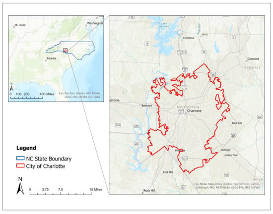
Figure 1.
Geographical location with call out of Charlotte, North Carolina, USA.
2.2. Data Sources
GIS tools (ArcGIS Pro 3.2.0, Esri, Redlands, CA, USA) and RStudio (version 2024.10.31, R version 4.4.2, RStudio PBC, Boston, MA, USA) were used to process and analyze spatial data to identify areas where enhanced vegetation could reduce noise pollution in Charlotte. There were two categories of data utilized for this study: dependent variable data (transportation noise exposure) and independent variables (vegetation coverage and population density). Population density data were obtained from Esri’s 2020 U.S. Census Block Groups dataset. Population density in this dataset represents the number of residents per unit of land area for each block group [29]. All spatial layers were projected to a common coordinate system: NAD83/North Carolina (ftUS).
2.2.1. Transportation Noise
Transportation noise data was obtained from the U.S. Department of Transportation’s National Transportation Noise Map [30]. The 2020 transportation data layers provide a 24-h daily average for aviation, highway, and passenger and freight rail. Noise monitors are located at Charlotte Douglass Airport (aviation). Road noise sources were modeled using average annual daily traffic values using average speeds, and road types for medium and heavy trucks, and automobiles, based on State-provided data from the Highway Performance Monitoring System. Rail noise included freight, passenger, transit (e.g., street cars and light rail), and included rail horns within ¼ mile of grade crossings. Noise levels below 45 dBA were excluded from the data for all noise types, and noise receptors were modeled at a resolution of 30 m at a height of 1.5 m. A threshold of 85 dBA was selected to define high-noise transportation zones because exposure to noise at or above this level has been linked with increased risks of noise-induced hearing loss and other adverse health outcomes in urban populations exposed to transportation noise [31]. Idling noises were also excluded from analysis, and hard ground areas (e.g., pavement or water) were reported as potentially being under-predicted. A full list of assumptions is provided in the documentation manual [32]. For statistical modeling, transportation noise exposure values from the DOT noise map (reported as A-weighted 24-h equivalent sound levels at 30 m resolution) were spatially averaged to the census block group level to produce a continuous dependent variable. In addition, areas exceeding 85 dBA were classified as high-noise zones for interpretive mapping.
2.2.2. Vegetation
Vegetation coverage was derived from the NDVI, which measures the density of green vegetation based on the difference between near-infrared and red reflectance. NDVI was calculated from Landsat 8 imagery (30-m resolution) acquired on 22 August 2020, downloaded from the U.S. Geological Survey’s Earth Explorer [33]. The selected image contains no cloud cover, and August represents peak vegetation in Charlotte, providing a representative snapshot of urban green space for the analysis. To quantify the spatial distribution of vegetation, NDVI data were processed to extract green space classes, with Class 3 (NDVI 0.266–0.337) representing medium vegetation, and Class 4 (NDVI 0.338–0.549) representing dense vegetation. The percentage of vegetation cover was then calculated for each census block group. The overall NDVI values in the study area ranged from −0.038 to 0.549. This vegetation layer, along with block group population density and transportation noise exposure data described in the methodology, provided the basis for subsequent spatial statistical modeling.
2.2.3. Variable Construction
For each census block group, three key variables were constructed to support spatial modeling. First, vegetation coverage was calculated by summing the area of medium and dense vegetation, as indicated by the NDVI classification, within each block group and expressing it as a percentage of the total block group area. Second, the Euclidean distance to the nearest high-noise zone (85 dBA) was computed from the geometric centroid of each block group to the nearest high-noise polygon, and block group population density (PopDen) was included as an additional variable in the spatial dataset. Although distance does not directly represent acoustic exposure, because sound propagation in urban areas is shaped by factors such as urban structure, physical obstructions, terrain, and characteristics of the noise source, Euclidean distance to high-noise zones was employed as a practical proxy for relative exposure. These variables were integrated into a unified spatial dataset, forming the foundation for subsequent statistical modeling of the relationships between green space coverage, noise exposure, and population distribution.
2.3. Statistical Analysis
2.3.1. Ordinary Least Squares (OLS) Regression and Spatial Autocorrelation Testing
Ordinary Least Squares (OLS) regression was initially applied to examine the relationships between noise exposure, population density, and vegetation coverage. The OLS model provides global estimates of regression coefficients across the study area. The dependent variable was the minimum distance from each block group to the nearest high-noise area (), while the independent variables included the percentage of medium and dense vegetation () and population density (). Regression coefficients () and the error term () were estimated globally [34,35].
Because OLS does not account for spatial variation in relationships [36], residuals were tested for spatial autocorrelation using Global Moran’s I to assess whether values were clustered, dispersed, or randomly distributed [37,38]. Significant spatial autocorrelation indicates unmodeled spatial dependencies, justifying the use of spatially explicit models such as the Spatial Autoregressive (SAR) model and Geographically Weighted Regression (GWR) to capture nonlinear effects and localized patterns [39,40]. Full methodological details, including the OLS and Moran’s I calculations and results are provided in the Supplementary Material (Figure S1).
2.3.2. Spatial Autoregressive (SAR) Model
Significant spatial autocorrelation in the OLS residuals (Moran’s I test) motivated the use of a Spatial Autoregressive (SAR) model for global estimation, while evidence of spatial non-stationarity in the vegetation–noise relationship motivated the additional use of Geographically Weighted Regression (GWR) to map local variation in coefficients.
The Spatial Autoregressive (SAR) model is a global spatial econometric model that incorporates spatial dependence directly into the regression structure by introducing a spatially lagged dependent variable. This model accounts for the influence that neighboring spatial units exert on each other, which is particularly useful when residual spatial autocorrelation is detected in an OLS model [41]. The SAR model is specified as follows:
where:
is the dependent variable (distance to high noise areas),
is the spatial autoregressive coefficient capturing the strength and direction of spatial dependence,
is the spatial weight matrix defining the spatial relationships between units,
is the matrix of independent variables (vegetation percentage and population density),
is the vector of regression coefficients, and
is the random error term.
This model accounts for spatial spillover effects, improving estimation accuracy when spatial dependencies are present.
2.3.3. Geographically Weighted Regression (GWR)
Geographically Weighted Regression (GWR) is a local spatial analysis method proposed by Brunsdon et al., 1996, designed to capture spatial heterogeneity in relationships between dependent and independent variables [42]. Unlike global models such as OLS or SAR, GWR allows regression coefficients to vary over space, providing localized estimates of parameter values at each observation point. The GWR model takes the form [43]:
where:
is the dependent variable for spatial unit i (distance to high noise areas),
are the explanatory variables (vegetation percentage and population density),
and are location-specific intercepts and coefficients estimated at the spatial coordinates of unit , and,
is the random error term.
The model parameters are estimated using a locally weighted least squares approach, where the weight assigned to each observation decreases with increasing distance from the target location. A Gaussian kernel function was applied to define the spatial weights:
where:
is the spatial weight between observation points i and j,
is the Euclidean distance between these points, and
is the bandwidth parameter controlling the spatial extent of local influence.
To capture spatial variation in the relationship between vegetation, population density, and noise exposure, multiple spatial regression models were applied. An Ordinary Least Squares (OLS) model was first used to assess overall trends, followed by Spatial Lag (SAR) and Spatial Error (SEM) models to address spatial dependence. Finally, a Geographically Weighted Regression (GWR) model was implemented to explore local variation across the study area. Lastly, model performance was evaluated using standard diagnostics, including the Akaike Information Criterion (AIC), residual spatial autocorrelation, and predictive accuracy (Table S1, Supplementary Material). While the SAR model captured global patterns and a nonlinear vegetation threshold, it missed local variation. The GWR model, used for final interpretation, revealed spatially varying effects of vegetation and population density on noise exposure. The optimal bandwidth for the GWR model was determined based on the corrected AIC (AICc), ensuring a balance between model complexity and fit [36,44,45]. For visualization, GWR coefficient and local R2 surfaces were classified into six equal-interval categories.
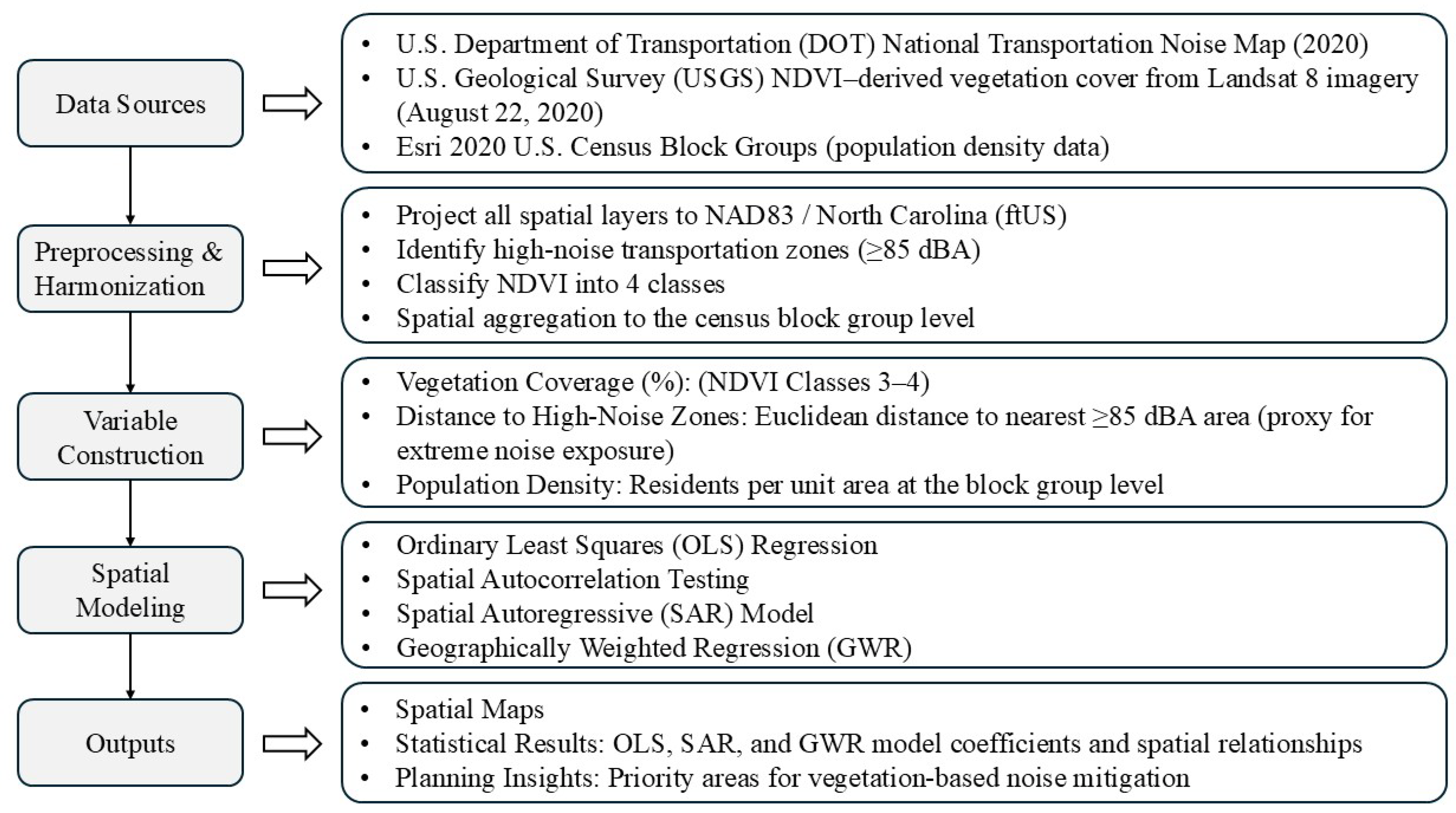
The study employed a multi-step analytical workflow that integrated transportation noise, vegetation, and population datasets into spatial models to quantify global and local associations (Figure 2).
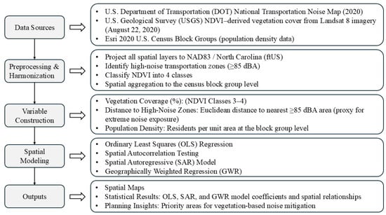
Figure 2.
Methodological workflow illustrating data sources, preprocessing steps, spatial modeling procedures, and analytical outputs used in the study.
3. Results
3.1. Spatial Patterns of Noise Exposure, Population and Vegetation Density
High transportation noise levels in Charlotte are concentrated near road networks and railway corridors (Figure 3a), with the highest recorded noise levels on the westside near Charlotte Douglas International Airport. Despite the high noise levels in the airport’s vicinity (west Charlotte), the population density in this area is low (Figure 3b). This highlights the significant impact of the transportation system on the urban acoustic environment. These observations emphasize the need for noise mitigation strategies that account for both the characteristics of the built environment and the spatial performance of vegetation. Following this, the NDVI map was used to identify and calculate the percentage of vegetation within each block group, providing insights into the spatial distribution of green coverage across the study area (Figure 3c,d).
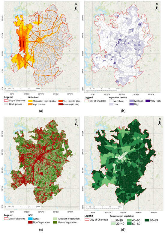
Figure 3.
(a) High noise levels, measured by decibels, are concentrated in West Charlotte, by the airport; (b) spatial distribution of population density across Charlotte, NC; (c) NDVI-derived vegetation coverage; (d) Block groups with the percentage of vegetation.
3.2. Global Relationship Between Population Density, Vegetation, and Noise Exposure
An initial OLS regression was used to assess the global relationships between population density, vegetation coverage, and distance to high-noise areas (≥85 dB). Results indicated a weak but statistically significant positive relationship between population density and distance to high-noise zones (β = 0.08, p < 0.05), suggesting that more densely populated block groups are generally located farther from high-noise areas, likely influenced by the low-population zones surrounding Charlotte Douglas International Airport (Figure S1a). Vegetation cover also showed a positive association with distance to high-noise areas, consistent with the buffering effect of green spaces (Figure S1b). However, the OLS model explained only a small portion of variance (R2 = 0.07), and residuals exhibited strong spatial autocorrelation (Moran’s I = 0.61, p < 0.001), indicating that spatial dependencies and non-stationarity are present. These findings emphasize the limitations of global OLS models in capturing the complex spatial patterns of noise exposure and motivate the use of spatially explicit models such as SAR and GWR. Full details of the OLS results, including regression specifications and confidence intervals, are provided in the Supplementary Material (Figure S1).
3.3. Spatial Autocorrelation, Nonlinear Vegetation Effects, and Model Improvement: Spatial Autoregressive (SAR) Model
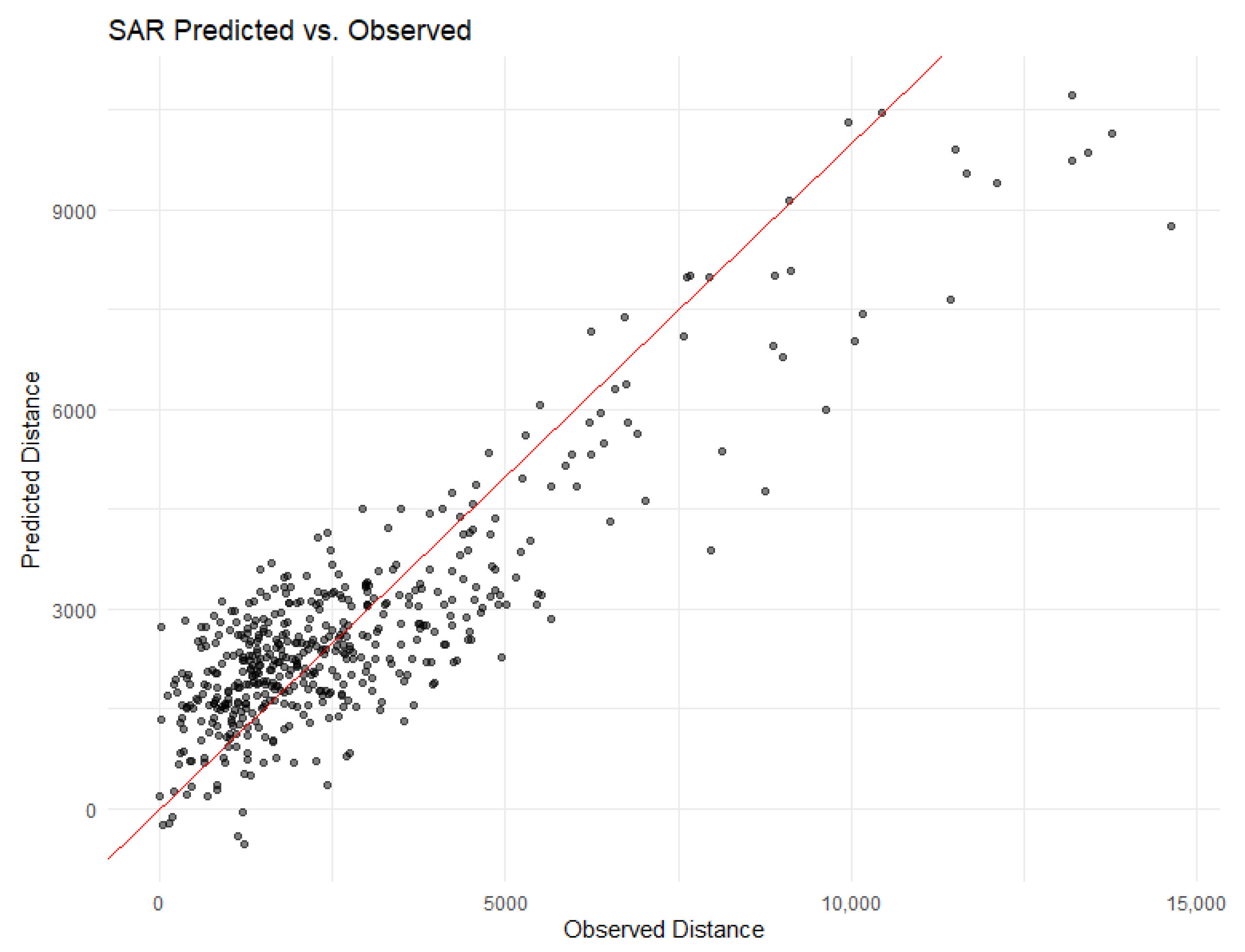
The Spatial Autoregressive (SAR) model with a quadratic vegetation term demonstrated superior performance, effectively accounting for spatial dependency and nonlinear vegetation effects. The SAR model significantly improved model fit compared to the OLS model, with an Akaike Information Criterion (AIC) of 8476.5 and a Root Mean Squared Error (RMSE) of 1174.7 m, while eliminating residual spatial autocorrelation. The predictive accuracy of the SAR model had a strong alignment between observed and predicted distances to high noise zones (Figure 4).
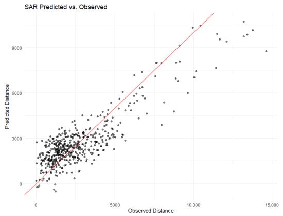
Figure 4.
Spatial Autoregressive (SAR) Model Performance showing Predicted vs. Observed Distances to High Noise Zones (≥85 dB).
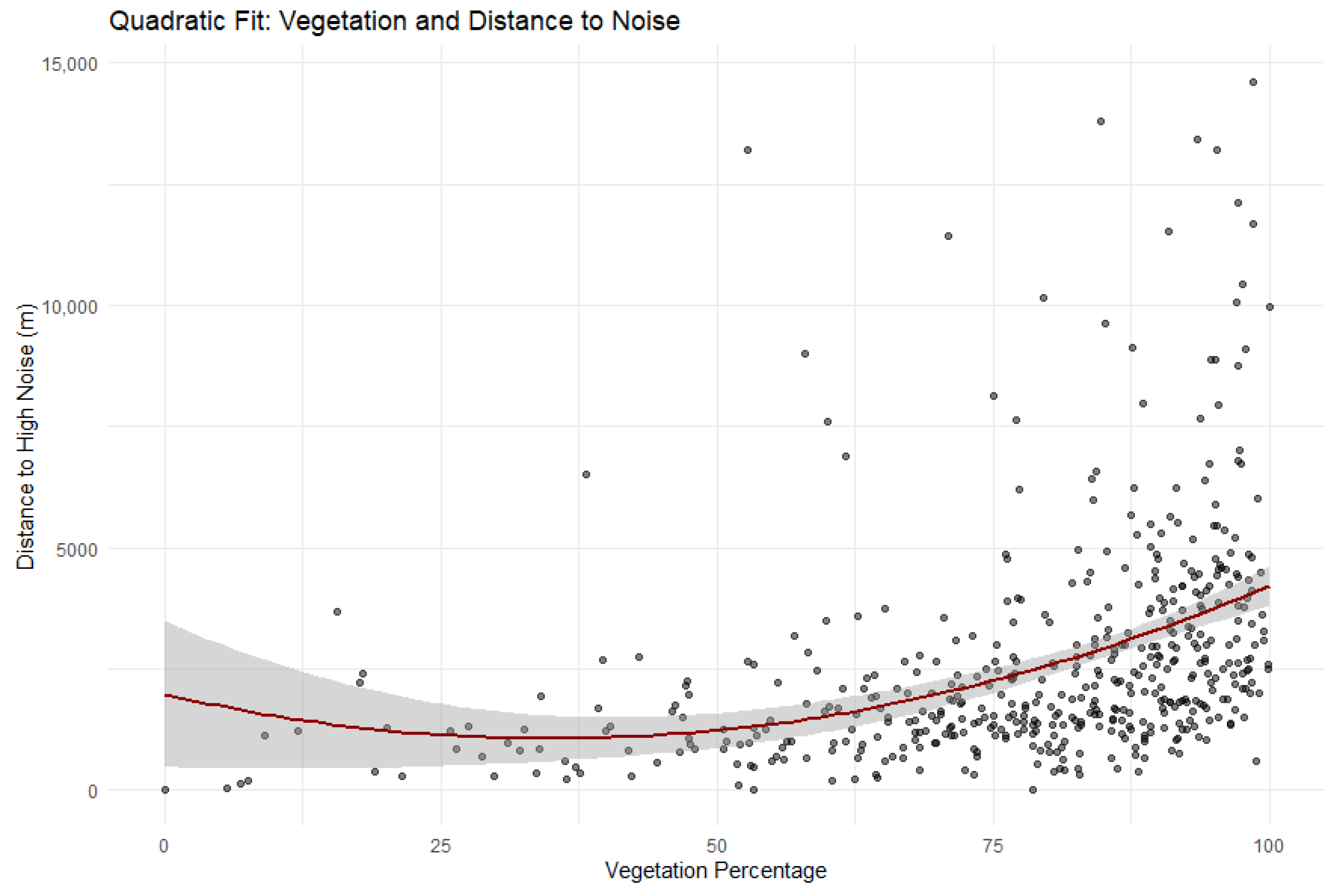
Results from the SAR model revealed a statistically significant vegetation threshold at 35.2% vegetation coverage, beyond which the noise-buffering effect of vegetation became substantially stronger. This threshold was derived from the vertex of the quadratic vegetation term in the SAR model, representing the point at which the marginal increase in distance to high-noise areas (≥85 dB) begins to accelerate. To account for uncertainty, sensitivity analyses were conducted by varying the vegetation percentage in 1% increments and assessing changes in predicted distances, which showed that the threshold consistently fell within the range of 34–36% across model specifications. Below this threshold, the impact of vegetation on increasing distance to high noise exposure areas (≥85 dB) was negligible; however, once vegetation exceeded this critical mass, its mitigating effect on noise exposure became markedly more pronounced. This nonlinear relationship was modeled by a quadratic fit curve capturing the threshold dynamics (Figure 5). These findings align with prior research emphasizing threshold dynamics in vegetation’s capacity to reduce environmental noise, especially through dense canopy coverage [24].
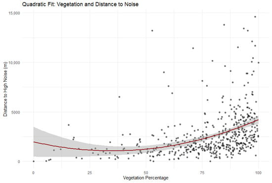
Figure 5.
Nonlinear Relationship Between Vegetation Coverage and Distance to High Noise Areas using a quadratic fit.
3.4. Spatial Heterogeneity and Localized Effects: Geographically Weighted Regression (GWR)
The GWR model revealed substantial spatial heterogeneity in the strength and direction of vegetation’s influence on distance to high-noise areas. NDVI-derived vegetation percentages varied considerably across the city, with higher concentrations typically found in suburban and southeastern regions (Figure 3d). Local GWR coefficients for vegetation ranged from near zero to over 300 m, indicating that vegetation’s effect on buffering noise exposure was highly context-dependent. The strongest positive effects were concentrated in the southern and eastern regions of the county, where denser tree canopy and vegetation coverage effectively increased the distance between residential areas and noise sources (Figure 6). The spatial variation in vegetation’s effect was consistent with the nonlinear threshold identified in the SAR model.
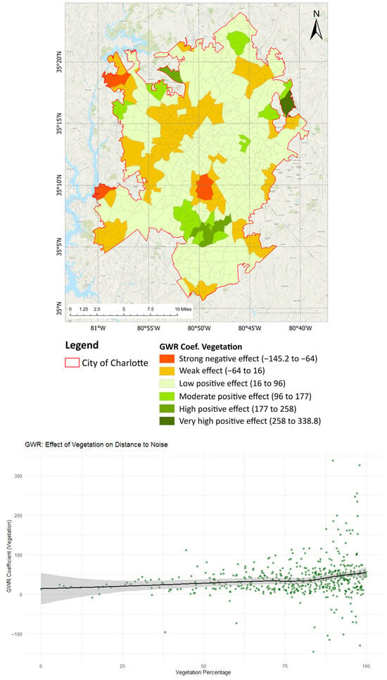
Figure 6.
GWR coefficients for the vegetation effect on distance to high-noise areas. Coefficients are classified into six equal-interval categories ranging from −145.2 to 338.8. Positive values indicate areas where vegetation is associated with increased distance from noise, while negative values indicate areas with reduced effectiveness.
The GWR analysis revealed substantial spatial heterogeneity in vegetation effects on noise buffering, with coefficients ranging from −145.2 to 338.8 and a median value of 34.6, indicating strong localized mitigation in many areas. Positive coefficients indicate areas where higher vegetation coverage is associated with increased distance to high-noise zones, reflecting effective local noise mitigation. Conversely, negative coefficients suggest locations where vegetation is correlated with shorter distances to noisy areas, potentially due to complex urban contexts such as vegetation clustering near roads or industrial zones, where trees do not buffer but may coexist with high-noise sources. The large magnitude of some coefficients likely reflects block groups with unusually high or low vegetation coverage relative to their surroundings, amplifying the localized effect in the GWR model.
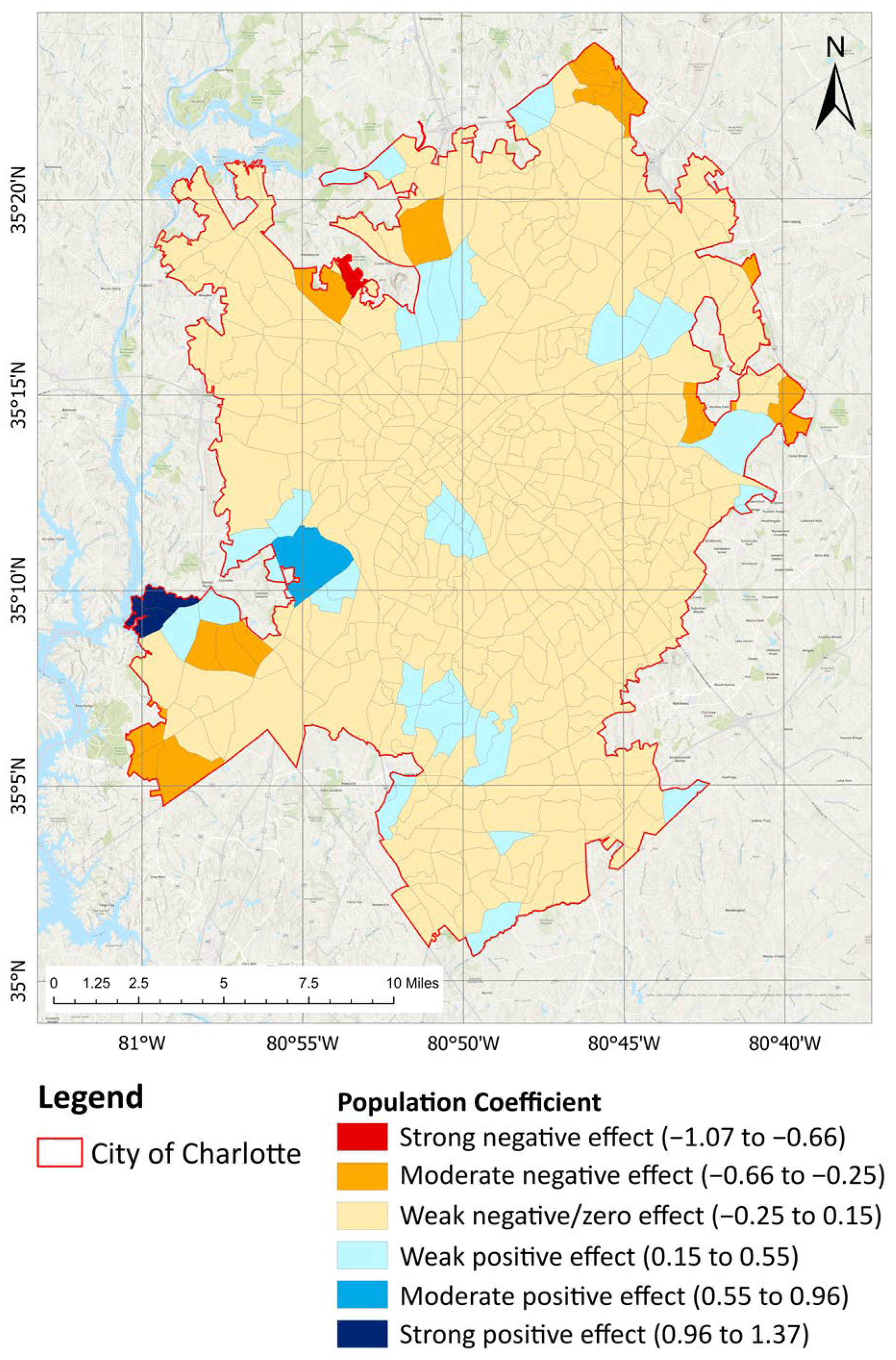
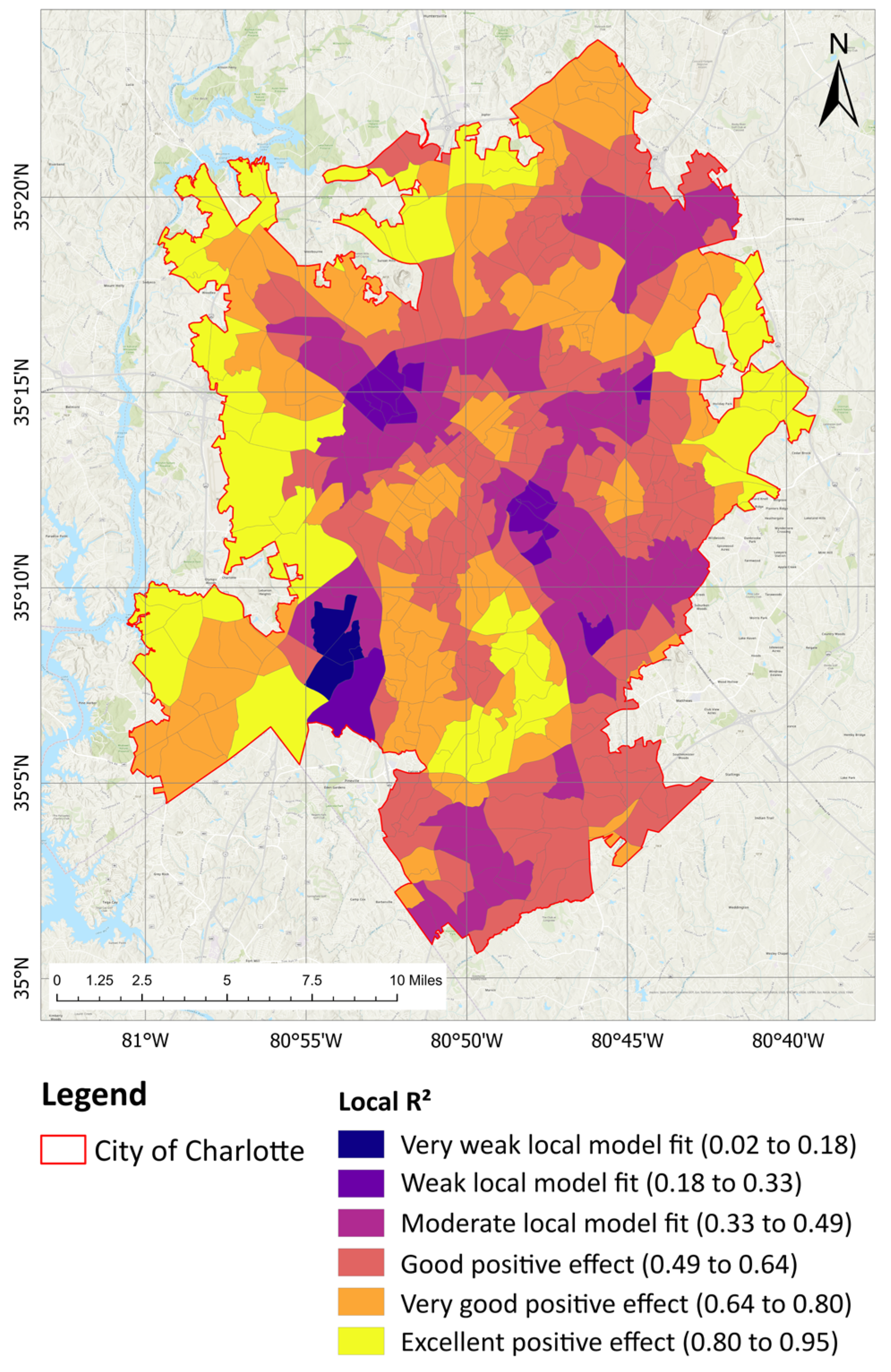
Population density effects varied from −1.07 to 1.37, with a median close to zero, reflecting more nuanced spatial patterns. In some southwestern block groups, higher population density corresponds with greater noise exposure, while in most areas, the effect is weak or inverse. These findings underscore the importance of interpreting GWR coefficients within their local context, as the direction and strength of associations can differ substantially across the city (Figure 6 and Figure 7). Population density exhibited significant localized effects in select southwestern block groups but was not a consistently strong predictor across the entire study area (Figure 7). Local R2 values from the GWR model ranged from 0.02 to 0.95, demonstrating good model performance and reinforcing that both vegetation and population density influence noise exposure in a spatially heterogeneous manner (Figure 8).
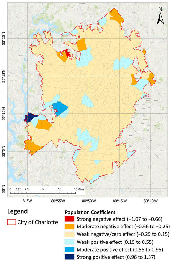
Figure 7.
GWR coefficients for population density affect distance to high-noise areas. Coefficients are classified into six equal-interval categories ranging from −1.0 to 1.3. Positive values indicate areas where higher population density is associated with greater distance from noise, while negative values indicate areas where higher population density is associated with reduced distance to noise.
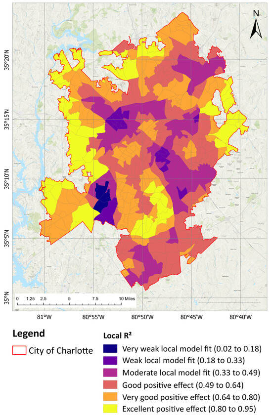
Figure 8.
Local R2 values from the Geographically Weighted Regression (GWR) model, classified into six equal-interval categories ranging from 0.02 to 0.95. Higher R2 values (yellow areas) indicate locations where vegetation coverage and population density more strongly explain spatial variation in distance to high-noise zones, highlighting substantial spatial heterogeneity in model performance across Charlotte.
3.5. Identification of Priority Areas for Green Infrastructure Intervention
Building on the GWR and SAR model findings, a three-tier classification system was developed to spatially target green space improvements across Charlotte (Figure 9). This system incorporated three criteria: vegetation coverage, proximity to high-noise zones, and the effectiveness of vegetation in mitigating noise, as captured by local GWR coefficients.
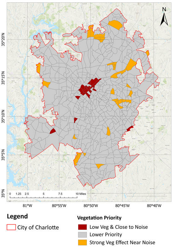
Figure 9.
Priority Areas for Vegetation Improvement in Charlotte. Dark Red indicates census block groups with lower vegetation (<35.2%) in proximity to high transportation noise, while Orange census block groups are in high transportation noise zones with existing green space.
- 1.
- Low Veg and Close to Noise (Dark Red):
Block groups with vegetation coverage below 35.2%, located within the lowest 30% of distances to high-noise zones (typically <1500 m), and exhibiting weak or negligible vegetation coefficients (bottom 20%). These areas represent critical intervention zones where residents are directly exposed to elevated noise levels and lack sufficient green space.
- 2.
- Strong Veg Effect Near Noise (Orange):
Areas near high-noise sources that exhibit high positive vegetation coefficients (top 30%) indicate that existing vegetation is already providing effective noise mitigation. These areas should be prioritized for preservation and potential expansion of vegetation buffers.
- 3.
- Lower Priority Areas (Gray):
The remaining block groups possess moderate to high vegetation coverage, greater distances from major noise sources, or weak vegetation-noise relationships. While not immediate targets for intervention, these zones may benefit from long-term planning as urban development progresses.
This spatially explicit, data-driven classification provides a practical framework to guide targeted vegetation enhancement and urban noise resilience strategies. By integrating vegetation thresholds, spatial heterogeneity, and proximity to noise sources, the approach supports evidence-based, place-specific green infrastructure planning to reduce noise exposure and promote healthier urban environments.
3.6. Statistical Summary of Model Performance
The Spatial Autoregressive (SAR) model with a quadratic vegetation term provided the best overall model fit, effectively capturing both spatial dependency and the nonlinear influence of vegetation on noise exposure (Table 1). The quadratic term for vegetation was highly significant ( < 0.001), confirming a nonlinear relationship wherein noise-buffering effects of vegetation increase substantially beyond 35.2% coverage. The spatial lag term ( = 0.893, < 0.001) highlights strong spatial dependence, underscoring the need for a spatially explicit modeling approach.

Table 1.
Coefficient Estimates for Best-Fitting SAR Model with Quadratic Vegetation Term.
Model comparison results (Table S1, Supplementary Material) indicate the superior performance of the SAR model. The SAR with a quadratic vegetation term achieved the lowest AIC (8476.5) and RMSE (1174.7 m), while effectively removing residual spatial autocorrelation. Although GWR does not provide global fit statistics, it revealed pronounced local variation in vegetation and population density effects. These insights are crucial for spatially targeted noise mitigation. Overall, the SAR model best captures global spatial processes and nonlinear vegetation effects, whereas the GWR model highlights local dynamics essential for guiding green infrastructure interventions across Charlotte.
4. Discussion
This study underscores the critical yet spatially heterogeneous role of urban vegetation in mitigating transportation noise exposure across Charlotte, North Carolina. By integrating Ordinary Least Squares (OLS), Spatial Autoregressive (SAR), and Geographically Weighted Regression (GWR) models, this research advances the spatial analysis of urban acoustic environments beyond traditional global approaches. The findings reveal that the relationship between vegetation cover and noise exposure is nonlinear, with a threshold at 35.2% vegetation coverage, beyond which the benefits of noise attenuation increase significantly. This critical insight supports previous findings [19,24] that highlight the importance of vegetation density and structure in enhancing noise mitigation, but this study contributes new empirical evidence by quantifying this threshold within a U.S. urban context, rather than relying on qualitative or generalized assumptions about green space presence.
Compared to other studies that primarily emphasize the presence or absence of green space [21,22], this research offers a novel threshold-based approach and integrates spatial heterogeneity through GWR modeling. The GWR results revealed substantial local variation in vegetation’s influence on noise buffering, with local R2 values ranging from 0.02 to 0.95 and coefficients exceeding 300 m in some areas. These spatial patterns confirm that the effectiveness of noise mitigation is not uniform, but rather contingent upon local vegetation characteristics, urban form, and proximity to major transportation corridors. Stronger vegetation effects in southern and eastern Charlotte likely reflect lower highway densities, reduced freight and commuter corridor intensity, and more continuous residential tree canopy, enhancing vegetation’s acoustic buffering capacity. In contrast, corridors surrounding Charlotte Douglas International Airport exhibit diminished vegetation effects due to persistent aviation noise and limited continuous canopy coverage. This variability is further exhibited by the outcomes from the global OLS model, which indicated a general positive association between vegetation percentage and noise-buffering distance, versus the GWR, which revealed stronger local effects in areas where vegetation coverage exceeded approximately 35.2%, reinforcing the presence of a critical vegetation threshold for effective noise mitigation in Charlotte’s urban context (Figure 6). Together, the SAR and GWR models provide complementary insights. While the SAR model identifies a significant global relationship between vegetation and noise exposure, confirming that vegetation contributes to noise attenuation city-wide, the GWR model reveals substantial spatial variation in this association, showing where these relationships intensify, weaken, or reverse. This integrated global–local perspective demonstrates that vegetation–noise dynamics cannot be fully understood from either scale alone, and that planning interventions require attention both to general city-wide tendencies and to localized spatial heterogeneity.
By contrast, block groups in the urban core and northern transport corridors exhibit weaker mitigation effects due to multilane arterials, higher traffic volumes, and fragmented green space patterns that limit the propagation and acoustic effectiveness of vegetative buffers. These spatial patterns indicate that transportation morphology and land-use composition modulate the functional capacity of vegetation to reduce noise exposure. However, these spatially varying relationships highlight the need for place-based analyses, as noise–vegetation interactions may differ across cities with distinct urban morphologies, climates, and transportation systems.
Notably, lower population density areas near Charlotte Douglas International Airport consistently exhibited high noise levels, while densely populated areas in closer proximity to roadways showed elevated noise exposure and limited vegetation cover, signaling critical zones for targeted intervention. These patterns reflect the combined influence of transportation infrastructure, land-use zoning, and historical development, and suggest that vegetation alone cannot fully offset noise impacts in areas dominated by major noise sources such as airports and freight corridors. The three-tier classification framework developed in this study, based on vegetation percentage, proximity to noise, and mitigation effectiveness, offers a practical and replicable tool for prioritizing green infrastructure investments targeting transportation.
The novelty of this work lies in its integration of spatial regression techniques (SAR and GWR) with remote sensing-derived NDVI data, applied at the census block group level. This multi-scalar, spatially explicit approach enables a deeper understanding of where and how vegetation most effectively contributes to urban acoustic health. Moreover, by establishing a quantifiable vegetation threshold and identifying priority intervention zones, the study bridges the gap between ecological understanding and actionable urban planning.
5. Conclusions
In conclusion, this research contributes to the growing body of literature advocating for nature-based solutions to urban environmental challenges by demonstrating that vegetation mitigates transportation noise in a nonlinear and spatially heterogeneous manner. The identification of a 35.2% vegetation coverage threshold provides a concrete planning reference point for Charlotte, while also highlighting that effective noise mitigation requires more than minimal or fragmented green space.
The applicability of this threshold should be interpreted with caution. Climatic conditions, vegetation structure, urban morphology, and transportation intensity vary across cities, and the specific threshold identified here is not intended to be universally transferable. Rather, the primary contribution lies in the methodological framework used to identify region-specific vegetation thresholds, which can be adapted and applied in other urban contexts.
The integration of global and local spatial models demonstrates that vegetation effectiveness depends not only on overall coverage but also on spatial configuration and surrounding land-use characteristics. This insight emphasizes the importance of targeted, place-based green infrastructure strategies rather than uniform citywide interventions. The priority-area classification developed in this study offers a data-driven approach to guide such interventions, supporting more efficient and equitable allocation of resources.
Several limitations should be acknowledged. The analysis relies on modeled transportation noise data rather than long-term field measurements, and NDVI captures vegetation quantity but not structural attributes such as canopy height or species composition. Additionally, the cross-sectional design does not capture temporal changes in vegetation or noise exposure. Using Euclidean distance to high-noise zones as a proxy for exposure also simplifies the complex ways sound propagates in urban environments. Future research should incorporate longitudinal noise monitoring, detailed vegetation structure metrics, and explicit links to public health and environmental equity outcomes.
Overall, this study demonstrates that integrating spatial econometric modeling with remote sensing data can substantially improve understanding of urban noise dynamics. By identifying where vegetation is most effective, how much is needed, and under what conditions it provides meaningful benefits, the framework presented here offers valuable guidance for urban planners and policymakers seeking to design more livable and acoustically resilient cities.
Supplementary Materials
The following supporting information can be downloaded at: https://www.mdpi.com/article/10.3390/su18031476/s1, Figure S1: (a) OLS Regression of Population Density against distance to noise levels greater than or equal to 85 decibels (dBA); (b) OLS Regression of Vegetation Coverage on Distance to High Noise Exposure Areas (≥85 dB) in Charlotte, NC; Table S1: Model Comparison Summary.
Author Contributions
Conceptualization, P.M. and F.-A.H.; methodology, P.M. and F.-A.H.; software, P.M.; validation, P.M. and F.-A.H.; formal analysis, P.M.; investigation, P.M.; resources, P.M.; data curation, P.M.; writing—original draft preparation, P.M.; writing—review and editing, P.M. and F.-A.H.; visualization, P.M.; supervision F.-A.H.; project administration, F.-A.H. All authors have read and agreed to the published version of the manuscript.
Funding
This research received no external funding.
Institutional Review Board Statement
Not applicable.
Informed Consent Statement
Not applicable.
Data Availability Statement
The datasets generated during and/or analyzed during the current study are available from the corresponding author on reasonable request.
Conflicts of Interest
The authors declare no conflicts of interest.
Abbreviations
The following abbreviations are used in this manuscript:
| NDVI | Normalized Difference Vegetation Index |
| OLS | Ordinary Least Squares |
| SAR | Spatial Autoregressive |
| GWR | Geographically Weighted Regression |
| UDO | Unified Development Ordinance |
| AIC | Akaike Information Criterion |
| RMSE | Root Mean Squared Error |
References
- United Nations Department of Economic and Social Affairs. World Urbanization Prospects: The 2018 Revision; United Nations: New York City, NY, USA, 2018. [Google Scholar]
- Elmqvist, T.; Goodness, J.; Marcotullio, P.J.; Parnell, S.; Sendstad, M.; Wilkinson, C.; Fragkias, M.; Güneralp, B.; McDonald, R.I.; Schewenius, M.; et al. Urbanization, Biodiversity and Ecosystem Services: Challenges and Opportunities: A Global Assessment; Springer: Berlin/Heidelberg, Germany, 2013; 755p. [Google Scholar] [CrossRef]
- Puplampu, D.A.; Boafo, Y.A. Exploring the impacts of urban expansion on green spaces availability and delivery of ecosystem services in the Accra metropolis. Environ. Chall. 2021, 5, 100283. [Google Scholar] [CrossRef]
- Pandey, B.; Ghosh, A. Urban ecosystem services and climate change: A dynamic interplay. Front. Sustain. Cities 2023, 5, 1281430. [Google Scholar] [CrossRef]
- Paudyal, K.; Baral, H.; Bhandari, S.P.; Bhandari, A.; Keenan, R.J. Spatial assessment of the impact of land use and land cover change on supply of ecosystem services in Phewa watershed, Nepal. Ecosyst. Serv. 2019, 36, 100895. [Google Scholar] [CrossRef]
- Madadi, P.; Sadeghi, A. Integrating Urban Expansion and Flood Risk: A Spatial Assessment of Impervious Surface Growth and Floodplain Exposure in Mecklenburg County (2011–2021). World Water Policy 2025, 12, e70052. [Google Scholar] [CrossRef]
- Nguyen, M.H.; Nguyen, M.H.T.; Jin, R.; Nguyen, Q.L.; La, V.P.; Le, T.T.; Vuong, Q.H. Preventing the Separation of Urban Humans from Nature: The Impact of Pet and Plant Diversity on Biodiversity Loss Belief. Urban Sci. 2023, 7, 46. [Google Scholar] [CrossRef]
- Zhang, P.; Dong, Y.; Ren, Z.; Wang, G.; Guo, Y.; Wang, C.; Ma, Z. Rapid urbanization and meteorological changes are reshaping the urban vegetation pattern in urban core area: A national 315-city study in China. Sci. Total Environ. 2023, 904, 167269. [Google Scholar] [CrossRef]
- Hartig, T.; Mitchell, R.; De Vries, S.; Frumkin, H. Nature and health. Annu. Rev. Public Health 2014, 35, 207–228. [Google Scholar] [CrossRef]
- Wood, E.; Harsant, A.; Dallimer, M.; de Chavez, A.C.; McEachan, R.R.C.; Hassall, C. Not all green space is created equal: Biodiversity predicts psychological restorative benefits from urban green space. Front. Psychol. 2018, 9, 391823. [Google Scholar] [CrossRef]
- Xu, J.; Liu, N.; Polemiti, E.; Garcia-Mondragon, L.; Tang, J.; Liu, X.; Lett, T.; Yu, L.; Nöthen, M.M.; Feng, J.; et al. Effects of urban living environments on mental health in adults. Nat. Med. 2023, 29, 1456–1467. [Google Scholar] [CrossRef]
- Lackey, N.Q.; Tysor, D.A.; McNay, G.D.; Joyner, L.; Baker, K.H.; Hodge, C. Mental health benefits of nature-based recreation: A systematic review. Ann. Leis. Res. 2021, 24, 379–393. [Google Scholar] [CrossRef]
- Li, S.; Chen, T.; Chen, F.; Mi, F. How Does the Urban Forest Environment Affect the Psychological Restoration of Residents? A Natural Experiment in Environmental Perception from Beijing. Forests 2023, 14, 1986. [Google Scholar] [CrossRef]
- Hoover, F.-A.; Meerow, S.; Coleman, E.; Grabowski, Z.; McPhearson, T. Why go green? Comparing rationales and planning criteria for green infrastructure in U.S. city plans. Landsc. Urban Plan. 2023, 237, 104781. [Google Scholar] [CrossRef]
- McPhearson, T.; Kremer, P.; Hamstead, Z.A. Mapping ecosystem services in New York City: Applying a social–ecological approach in urban vacant land. Ecosyst. Serv. 2013, 5, 11–26. [Google Scholar] [CrossRef]
- Semeraro, T.; Scarano, A.; Buccolieri, R.; Santino, A.; Aarrevaara, E. Planning of Urban Green Spaces: An Ecological Perspective on Human Benefits. Land 2021, 10, 105. [Google Scholar] [CrossRef]
- Tzoulas, K.; Korpela, K.; Venn, S.; Yli-Pelkonen, V.; Kaźmierczak, A.; Niemela, J.; James, P. Promoting ecosystem and human health in urban areas using Green Infrastructure: A literature review. Landsc. Urban Plan. 2007, 81, 167–178. [Google Scholar] [CrossRef]
- Madadi, P.; Masnavi, M.R. Environmental planning of urban green infrastructure networks in the eco-city framework, the case of Ghare-Kahriz Arak, Iran. Discov. Cities 2025, 2, 92. [Google Scholar] [CrossRef]
- Feng, L.; Wang, J.; Liu, B.; Hu, F.; Hong, X.; Wang, W. Does Urban Green Space Pattern Affect Green Space Noise Reduction? Forests 2024, 15, 1719. [Google Scholar] [CrossRef]
- Munzel, T.; Gori, T.; Babisch, W.; Basner, M. Cardiovascular effects of environmental noise exposure. Eur. Heart J. 2014, 35, 829–836. [Google Scholar] [CrossRef]
- Zaman, M.; Muslim, M.; Jehangir, A. Environmental noise-induced cardiovascular, metabolic and mental health disorders: A brief review. Environ. Sci. Pollut. Res. 2022, 29, 76485–76500. [Google Scholar] [CrossRef]
- Stuhlmacher, M.; Woods, J.; Yang, L.; Sarigai, S. How Does the Composition and Configuration of Green Space Influence Urban Noise?: A Systematic Literature Review. Curr. Landsc. Ecol. Rep. 2024, 9, 73–87. [Google Scholar] [CrossRef]
- Margaritis, E.; Kang, J. Relationship between urban green spaces and other features of urban morphology with traffic noise distribution. Urban For. Urban Green. 2016, 15, 174–185. [Google Scholar] [CrossRef]
- Margaritis, E.; Kang, J. Relationship between green space-related morphology and noise pollution. Ecol. Indic. 2017, 72, 921–933. [Google Scholar] [CrossRef]
- Singh, K.K.; Vogler, J.B.; Shoemaker, D.A.; Meentemeyer, R.K. LiDAR-Landsat data fusion for large-area assessment of urban land cover: Balancing spatial resolution, data volume and mapping accuracy. ISPRS J. Photogramm. Remote Sens. 2012, 74, 110–121. [Google Scholar] [CrossRef]
- TreesCharlotte; PlanIT Geo. Charlotte, NC Urban Tree Canopy Assessment. 2023. Available online: https://treescharlotte.org/wp-content/uploads/2023/05/charlotte-nc-tree-canopy-assessment-report-final.pdf?utm_source=chatgpt.com (accessed on 24 May 2025).
- City of Charlotte. Urban Forestry. City of Charlotte. 2025. Available online: https://www.charlottenc.gov/Growth-and-Development/Getting-Started-on-Your-Project/Urban-Forestry?utm_source=chatgpt.com (accessed on 1 June 2025).
- City of Charlotte. Charlotte Tree Ordinance; City of Charlotte: Charlotte, NC, USA, 2023; Volume 1.
- Esri. U.S. Census Block Groups (2020). 2020. Available online: https://www.arcgis.com/home/search.html?restrict=false&sortField=relevance&sortOrder=desc&searchTerm=tags%3A%22+block+groups%22#content (accessed on 10 January 2025).
- U.S. Department of Transportation, B. of T.S. U.S. Department of Transportation, Bureau of Transportation Statistics. 2020. Available online: https://maps.dot.gov/BTS/NationalTransportationNoiseMap (accessed on 10 January 2025).
- Welch, D.; Shepherd, D.; Dirks, K.N.; Reddy, R. Health effects of transport noise. Transp. Rev. 2023, 43, 1190–1210. [Google Scholar] [CrossRef]
- Volpe National Transportation Systems Center: Environmental Measurement and Modeling Division, Environmental Science and Engineering Division. National Transportation Noise Map Documentation; United States Department of Transportation Office of the Assistance Secretary for Research and Technology Volpe National Transportation Systems Center Environmental Measurement and Modeling Division, Environmental Science and Engineering Division: Cambridge, MA, USA, 2020. [CrossRef]
- U.S. Geological Survey (USGS). USGS EarthExplorer. 2020. Available online: https://earthexplorer.usgs.gov/ (accessed on 15 January 2025).
- Barnes, J.C.; Forde, D.R. (Eds.) OLS (Linear) Regression. In The Encyclopedia of Research Methods in Criminology and Criminal Justice: Volume II: Parts 5–8; John Wiley & Sons, Inc.: Hoboken, NJ, USA, 2021; Volume 2, pp. 509–514. [Google Scholar] [CrossRef]
- Deilami, K.; Hayes, J.F.; Bechtel, B.; Keramitsoglou, I.; Kotthaus, S.; Voogt, J.A.; Zakšek, K.; Li, Z.; Thenkabail, P.S. Correlation or Causality between Land Cover Patterns and the Urban Heat Island Effect? Evidence from Brisbane, Australia. Remote Sens. 2016, 8, 716. [Google Scholar] [CrossRef]
- Jin, Y.; Zhang, H.; Yan, Y.; Cong, P. A Semi-Parametric Geographically Weighted Regression Approach to Exploring Driving Factors of Fractional Vegetation Cover: A Case Study of Guangdong. Sustainability 2020, 12, 7512. [Google Scholar] [CrossRef]
- Gedamu, W.T.; Plank-Wiedenbeck, U.; Wodajo, B.T. A spatial autocorrelation analysis of road traffic crash by severity using Moran’s I spatial statistics: A comparative study of Addis Ababa and Berlin cities. Accid. Anal. Prev. 2024, 200, 107535. [Google Scholar] [CrossRef]
- Zhang, C.; Lv, W.; Zhang, P.; Song, J. Multidimensional spatial autocorrelation analysis and it’s application based on improved Moran’s I. Earth Sci. Inform. 2023, 16, 3355–3368. [Google Scholar] [CrossRef]
- Dell’Anna, F.; Bravi, M.; Bottero, M. Urban Green infrastructures: How much did they affect property prices in Singapore? Urban For. Urban Green. 2022, 68, 127475. [Google Scholar] [CrossRef]
- Gao, C.; Feng, Y.; Tong, X.; Lei, Z.; Chen, S.; Zhai, S. Modeling urban growth using spatially heterogeneous cellular automata models: Comparison of spatial lag, spatial error and GWR. Comput. Environ. Urban Syst. 2020, 81, 101459. [Google Scholar] [CrossRef]
- Furková, A. Implementation of MGWR-SAR models for investigating a local particularity of European regional innovation processes. Cent. Eur. J. Oper. Res. 2022, 30, 733–755. [Google Scholar] [CrossRef]
- Brunsdon, C.; Fotheringham, A.S.; Charlton, M.E. Geographically Weighted Regression: A Method for Exploring Spatial Nonstationarity. Geogr. Anal. 1996, 28, 281–298. [Google Scholar] [CrossRef]
- Hu, M.; Li, Z.; Wang, J.; Jia, L.; Liao, Y.; Lai, S.; Guo, Y.; Zhao, D.; Yang, W. Determinants of the incidence of hand, foot and mouth disease in China using geographically weighted regression models. PLoS ONE 2012, 7, e38978. [Google Scholar] [CrossRef]
- Kupfer, J.A.; Farris, C.A. Incorporating spatial non-stationarity of regression coefficients into predictive vegetation models. Landsc. Ecol. 2007, 22, 837–852. [Google Scholar] [CrossRef]
- Wang, Q.; Ni, J.; Tenhunen, J. Application of a geographically-weighted regression analysis to estimate net primary production of Chinese forest ecosystems. Glob. Ecol. Biogeogr. 2005, 14, 379–393. [Google Scholar] [CrossRef]
Disclaimer/Publisher’s Note: The statements, opinions and data contained in all publications are solely those of the individual author(s) and contributor(s) and not of MDPI and/or the editor(s). MDPI and/or the editor(s) disclaim responsibility for any injury to people or property resulting from any ideas, methods, instructions or products referred to in the content. |
© 2026 by the authors. Licensee MDPI, Basel, Switzerland. This article is an open access article distributed under the terms and conditions of the Creative Commons Attribution (CC BY) license.


