Abstract
This study comprehensively considers soil formation factors such as land use types, soil types, depths, and geographical conditions in Lanxi City, China. Using multi-source public data, three environmental variable screening methods, the Boruta algorithm, Recursive Feature Elimination (RFE), and Particle Swarm Optimization (PSO), were used to optimize and combine 47 environmental variables for the modeling of soil pH based on the data collected from farmland in the study area in 2022, and their effects were evaluated. A Random Forest (RF) model was used to predict soil pH in the study area. At the same time, Pearson correlation analysis, an environmental variable importance assessment based on the RF model, and SHAP explanatory model were used to explore the main controlling factors of soil pH and reveal its spatial differentiation mechanism. The results showed that in the presence of a large number of environmental variables, the model with covariates selected by PSO before the application of the Random Forest algorithm had higher prediction accuracy than that of Boruta–RF, RFE–RF, and all variable prediction RF models (MAE = 0.496, RMSE = 0.641, R2 = 0.413, LCCC = 0.508). This indicates that PSO, as a covariate selection method, effectively optimized the input variables for the RF model, enhancing its performance. In addition, the results of the Pearson correlation analysis, RF-model-based environmental variable importance assessment, and SHAP explanatory model consistently indicate that Channel Network Base Level (CNBL), Elevation (DEM), Temperature mean (T_m), Evaporation (E_m), Land surface temperature mean (LST_m), and Humidity mean (H_m) are key factors affecting the spatial differentiation of soil pH. In summary, the approach of using PSO for covariate selection before applying the RF model exhibits high prediction accuracy and can serve as an effective method for predicting the spatial distribution of soil pH, providing important references for accurately simulating the spatial mapping of soil attributes in hilly and basin areas.
1. Introduction
Soil is formed by the combined effects of multiple factors, and its properties exhibit high spatial heterogeneity [1]. As one of the important chemical properties of soil, soil pH exhibits significant variability in its spatial distribution due to the comprehensive influences of various factors [2]. In addition, soil affects the existence and availability of soil nutrients, which are extremely important for soil fertility and plant growth [3,4]. Studying the spatial variation of soil pH and accurately grasping the detailed information of soil pH spatial distribution through reliable and effective prediction mapping is of great significance for the classification and utilization of soil, nutrient management, and scientific planning of land use [5,6].
Soil pH is the result of the combined effects of multiple factors during soil formation [7]. According to the principles of soil genesis, soil acidity and alkalinity are mainly influenced by climate, biology, parent materials, and human factors. Previous studies have found that soil organic matter and altitude are important factors driving soil pH changes, and rainfall and crop types have an impact on soil pH changes [8]. The traditional soil pH mapping method involves steps such as data collection, indoor prediction, field investigation, indoor interpretation, field verification, and boundary mapping, which are time-consuming and laborious. Digital soil mapping (DSM), grounded principally in the soil landscape model, capitalizes on the variances within soil landscape environments, including terrain and vegetation characteristics. The spatial distribution of soil properties is then inferred using GIS-based spatial analysis combined with mathematical algorithms. When juxtaposed with traditional soil mapping approaches, DSM exhibits distinct advantages, as elaborated in reference [9]. The prevalent DSM methodologies encompass linear regression, generalized linear regression, geostatistics, geographically weighted regression (GWR), fuzzy clustering, and Random Forest, among other techniques, as detailed in reference [10].
The use of statistical methods for digital soil mapping can achieve good results but cannot effectively handle the nonlinear relationship between environmental variables and soil properties. However, using machine learning methods for digital soil mapping can effectively solve this problem [11]. Recently, machine learning techniques have gained significant traction in the field of digital soil mapping. Various studies have reported on the use of machine learning models such as Random Forest (RF), Support Vector Regression (SVR), and Classification Regression Trees for digital soil mapping [12,13]. These methods have been employed in both domestic and international research to predict, classify, and simulate a variety of soil characteristics, including soil types, moisture, and other properties. For instance, Dharumarajan et al. [14] applied the RF model to predict soil organic carbon, pH levels, and soluble salt concentrations in southern India’s semi-arid tropical region. Their findings demonstrated that the RF model enhanced the accuracy of spatial predictions for soil attributes. Similarly, Chagas et al. showed that the RF model outperformed multiple linear regression in terms of prediction accuracy and its ability to prevent overfitting when mapping the spatial distribution of soil texture in semi-arid regions [15]. Due to the numerous environmental factors that affect soil properties, the more feature variables available for modeling, the greater the computational complexity of the prediction model. Moreover, when the number of selected feature variables exceeds the optimal number, there may be a decrease in prediction accuracy [16]. Selecting the optimal feature variables from numerous environmental features, establishing a better machine learning model, and effectively conducting digital soil mapping are problems that need to be solved, and feature selection in machine learning can effectively solve them. Studies have shown that feature variable selection is crucial for shortening model runtime and improving model accuracy. It is necessary to select a small and optimal feature set for modeling [17]. Chen et al. proposed that the RF algorithm can be applied for feature screening before being used in an SVR model, indicating that using the RF algorithm for feature variable selection is effective [18]. The Boruta algorithm, which is a feature selection technique built on the RF model, utilizes an all-relevant feature selection approach to assign importance scores to individual features. This allows the algorithm to assess the relevance of each feature in relation to the target variable [19]. This study selected Lanxi City, Zhejiang Province, China, as the research area, used GIS technology to extract multiple environmental factors, and aimed to predict soil pH values. It attempted to combine the Boruta algorithm, Recursive Feature Elimination, and Particle Swarm Optimization—three feature variable screening algorithms—with RF to establish a soil pH value prediction model in hilly basin areas represented by Lanxi City, as well as to conduct digital mapping. Additionally, Pearson correlation analysis, the RF model’s environmental variable importance evaluation, and the SHAP interpretation model were employed to assess the influence of environmental factors on soil pH values. This can provide a reference for how to combine machine learning methods with environmental variable selection for digital soil mapping research in hilly basin areas.
2. Materials and Methods
2.1. General Situation
Lanxi City is situated in the central and western regions of Zhejiang Province, with coordinates ranging from 29°1′20″ to 29°27′30″ N and 119°13′30″ to 119°53′50″ E. Covering an area of 1313 square km (Figure 1), the city experiences a subtropical monsoon climate with significant annual rainfall. The terrain features a hilly basin at the heart of Zhejiang, bordered by mountains to the northeast, rolling low hills to the southwest, and a flat plain in the center. The main soil types in the research area, classified according to the World Reference Base for Soil Resources (WRB), include Acrisols (red soil), Alisols (yellow soil), Leptosols (lithological soil), Fluvisols (tidal soil), and Anthrosols (paddy soil), with agricultural land being the dominant land use. The main crops cultivated in the research area include maize, sweet potato, rice, rapeseed, and soybean. Additionally, a wide variety of fruits and vegetables are also extensively grown.
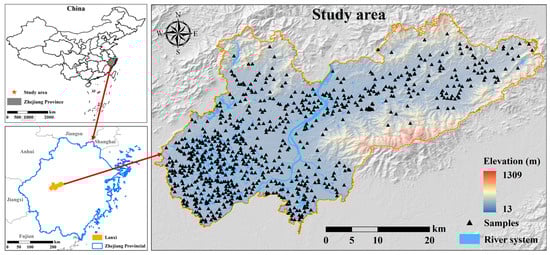
Figure 1.
Location of the research area and distribution of sampling points.
2.2. Sample Collection and Pretreatment
Surface soil samples were collected in 2022. All samples were exclusively collected from agricultural areas within the study region. Prior to field investigations, soil sampling points were pre-established using a grid sampling method. These points were systematically distributed across the study area based on field surveys to ensure a representative reflection of the spatial characteristics of soil properties in agricultural land. To ensure an adequate number of soil samples, a 2 × 2 km grid was systematically established within the study area, with sampling points positioned at the center of each grid cell to achieve uniform spatial distribution. Subsequent to this, grid points located outside agricultural zones were excluded using actual measurement data, and agricultural land layers were selected for preliminary screening. Given the intricate nature of agricultural landscapes, high-resolution Google Earth imagery was overlaid on the chosen grid points to visually assess land use types, aiding in the refinement of the selection process. Ultimately, a total of 1560 soil and crop samples were gathered. The soil sampling followed an upward drilling technique, with each sampling point surrounded by a 10 m × 10 m sub-grid. Soil cores were extracted from the top 0–20 cm of soil. At each location, ten soil cores were randomly obtained using a spiral soil auger with a 5 cm diameter and mixed thoroughly to form a composite sample. After fieldwork was completed, the soil samples were air-dried, ground, sieved through a 1.0 mm mesh, and stored in sealed glass jars for further analysis. Soil pH was then determined using the 1:5 soil-to-water extraction method [20,21].
2.3. Obtaining Environmental Covariates
The final database was painstakingly constructed, comprising 47 environmental variables (Table 1), with the soil pH value serving as the sole target variable. This suite of variables was judiciously selected to comprehensively encapsulate the diverse environmental factors that could potentially exert an influence on soil pH.

Table 1.
Input variables used in this study.
For the terrain data, 12.5 m Digital Elevation Model (DEM) data were employed. These data were procured from the NASA Earth Science Data website (https://www.earthdata.nasa.gov/, accessed on 15 February 2025). The selection of this data source was predicated on its high resolution and extensive coverage, enabling the precise capture of terrain features germane to the study area. All topographic factors, including slope, aspect, and elevation derivatives, were computed using GAGA-GIS 7.6.2 software. The default general parameter settings of this software, which have been extensively utilized and validated in analogous terrain-related investigations, were applied for terrain data processing. This ensured the reliability and comparability of the calculated topographic factors.
Climatic data, including annual mean temperature and precipitation, were obtained from the National Qinghai–Tibet Plateau Data Center in China (http://data.tpdc.ac.cn). This data center represents a comprehensive and authoritative platform for scientific data in the Qinghai–Tibet Plateau region. It operates a large-scale and long-term data collection and management system, furnishing high-quality climatic data that are eminently suitable for regional-scale environmental research. The data from this center have undergone rigorous quality control and calibration procedures, guaranteeing their accuracy and representativeness.
Remote sensing imagery was derived from Sentinel-2A satellite data available on the Google Earth Engine (GEE) public platform. With a spatial resolution of 10 m, Sentinel-2A imagery is well-suited for capturing detailed land surface features. To ensure consistency with field sampling, image acquisition was carefully aligned with the sampling period, and only cloud-free images were selected. This approach minimized potential distortions caused by cloud cover, ensuring that the remote sensing data accurately reflected surface conditions during the study. Soil texture information was sourced from the Geographic Remote Sensing Ecological Network Platform (www.gisrs.cn), which provides soil-related datasets with a spatial resolution of 900 m. This dataset was selected for its extensive coverage and reliable quality, as it integrates field surveys, laboratory analyses, and remote sensing techniques. By combining multiple data sources, the platform ensures that the soil texture data effectively represent the characteristics of the study area.
The soil type and land use data were derived from the measured data amassed during this experiment. This in-situ measurement approach was adopted to obtain highly accurate and site-specific data. The soil type data were ascertained through meticulous soil sampling and laboratory identification, while the land use data were collected through field mapping and remote-sensing interpretation. By leveraging the measured data, the study could better capture the local idiosyncrasies of soil type and land use, which are pivotal for comprehending their impacts on soil pH.
To facilitate subsequent modeling, the spatial resolution of the aforementioned selected environmental variables was resampled to 10 m using the ArcGIS 10.2 software. This resampling process was imperative to ensure that all variables exhibited a consistent spatial resolution, thereby enabling seamless integration within the modeling framework. Concurrently, their spatial extents and coordinate systems were standardized. The standardization of spatial extents was executed to ensure that all data encompassed the same geographical area, while the unification of coordinate systems was essential for precise spatial analysis and data alignment. These pre-processing steps were pivotal for ensuring the consistency and compatibility of the environmental variables within the analytical framework, thereby laying a solid foundation for accurate and reliable modeling outcomes.
2.4. Research Method
2.4.1. Random Forest
The Random Forest (RF) model is a tree-based ensemble learning approach capable of handling both classification tasks and the prediction of continuous variables [22]. One of its key advantages is that it does not require the dependent variable to follow a normal distribution or necessitate testing for multicollinearity among independent variables. More importantly, it effectively captures nonlinear relationships between predictor and response variables. In the RF model, the Bootstrap method is employed to randomly sample data with replacement from the original training set, generating m new training subsets. A Classification and Regression Tree (CART) model is independently constructed for each subset. Data points not included in the sampling process serve as out-of-bag (OOB) data. During tree construction, n independent variables are randomly selected at each node to determine the optimal split. The final prediction result is obtained through majority voting when dealing with categorical variables or by averaging the outputs in the case of continuous variables. To assess variable importance, RF measures the increase in mean square error (MSE) when a variable is excluded from the model’s predictions on OOB data, denoted as %IncMSE. A higher %IncMSE value indicates greater importance of the variable [23]. The RF model has two crucial parameters: the number of trees (ntree) and the number of predictor variables considered at each split (mtry). A larger ntree generally enhances model stability, provided computational resources allow it. The mtry parameter, which influences model performance, requires tuning through multiple trials, typically ranging from 1 to the total number of independent variables. In this study, the modeling and prediction of the RF model were implemented using the “random forest” package on the R studio 4.2.0 platform. This study used a grid search for parameter optimization, where the range of the number of random features (ntree) for split nodes was set to 10–1000, the step size was set to 10, and the number of decision trees (mtry) was set to 1–16 (taking one-third of the total number of variables) for modeling. The optimal parameters were determined based on the average R2 and RMSE results for ten-fold cross-validation. The results showed that the optimal ntree and mtry values for predicting pH were 200 and 15, respectively.
2.4.2. SHAP Interpretation Model
The RF model compensates for some of the shortcomings of traditional multiple linear regression models; it does not follow any assumptions and is insensitive to outliers, thus better solving the problem of multicollinearity and providing high-precision prediction results. Meanwhile, the model can effectively capture the complex nonlinear relationships between the dependent and independent variables by constructing multiple decision trees and integrating them through voting. In addition, the RF model can calculate the importance of variables, reveal the relative contributions of different independent variables to the dependent variable, and provide a reference for the screening and interpretation of environmental variables. However, in terms of interpretability, compared with multiple linear regression models, relying solely on the results of the model itself makes it difficult to intuitively explain the specific impact relationships between variables. A multiple linear regression model can quantify the effects of various influencing factors through regression coefficients, while the prediction results of the RF model rely on the comprehensive voting of multiple decision trees, and the measurement of the importance of variables is based on the number and contributions of tree splits. Therefore, although the RF model can evaluate the importance of variables, its internal decision rules are relatively complex, making it difficult to directly analyze the specific influencing mechanisms; thus, to some extent, there is a “black box” problem in machine learning. To address the issue of weak interpretability in RF models, this study uses the Shapley Additive Explanations (SHAP) method to compensate for the interpretability problem of RF models and visualize the real nonlinear effects between soil pH and environmental variables [24,25].
The SHAP method is based on cooperative game theory, and its core idea is to calculate the marginal contribution of feature observation points added to the model. The specific calculation method is as follows:
In the formula, is the SHAP value of feature ; is the feature subset used in the model; is the feature set in the model; is the number of features; is the prediction result of the model in the feature subset; is the predicted result for sample is the average of predicted values from other samples; is the SHAP value of sample at feature ; is the number of features. The SHAP value is an additional feature attribution method that interprets the predicted value of the model as the sum of the attribution values of each input feature. Therefore, a positive or negative value expresses the specific impact of different feature indicators in the study area on the prediction results.
2.4.3. Boruta Algorithm
Unrelated or redundant variables in a dataset often reduce the performance of ML algorithms. As a data preprocessing strategy, variable selection has been proven to be an effective way to reduce the dimensionality of the feature space by identifying the subset that contributes the most to the target variable or output from the original variable set. Variable selection helps to construct predictive models without correlated variables, biases, and unwanted noise, significantly improving prediction accuracy and reducing overfitting and training time [26,27]. The Boruta algorithm is a variable selection method based on a Random Forest model that can effectively identify and remove noisy variables in input features through multiple repeated operations. Firstly, the Boruta algorithm adds additional randomness to the original variables by creating shadow variables, then trains a Random Forest classifier on an extended dataset, and evaluates the importance of each variable [28,29]. The Boruta algorithm is a fully correlated environmental variable screening method that attempts to find all variables related to the target variable, which is beneficial for better understanding the relationship between the predictor variable and the target variable, rather than constructing a black-box prediction model with good prediction accuracy [30]. Due to its foundation of multiple Random Forest operations and evaluation of input features through statistical testing, it is relatively conservative in feature deletion and less likely to lose important information.
2.4.4. Recursive Feature Elimination
Recursive Feature Elimination (RFE) is a wrapper-based environmental variable filtering algorithm that recursively reduces the size of the feature set to select the subset of features that are most helpful for model prediction. The core idea of RFE is to build a model that can evaluate the contribution of each feature to the model’s predictive ability and gradually remove the least important features based on this until the required number of features is reached. The Recursive Feature Elimination method can efficiently screen some variables in the presence of relevant predictive factors, providing the prediction model with good prediction accuracy and making it suitable for research with a large number of environmental variables [31].
The main steps include the following: First, the model is trained using all available features to train it. The commonly chosen models are those that can provide feature importance ratings, and this study chose the support vector machine (SVM) model. Secondly, the importance of features is calculated. After the model training is completed, the importance of each feature is calculated based on the characteristics of the model. Again, based on the calculated importance, the least important features (i.e., the features that contribute the least to the model prediction) are removed. After removing one or more features, the model is retrained with the remaining features, and the above steps are repeated. This process is recursive, with each iteration removing some of the least important features until a predetermined number of features or a performance metric is reached. Finally, the RFE algorithm selects a feature subset that reduces the number of features while maintaining or improving the predictive performance of the model as much as possible.
2.4.5. Particle Swarm Optimization
Particle Swarm Optimization (PSO) is a global optimization algorithm proposed by Kennedy and Eberhart and inspired by swarm intelligence and the foraging behavior of bird flocks [32]. In recent years, PSO has been widely used in variable combination optimization problems, especially in environmental variable selection tasks for high-dimensional complex data. PSO initializes the position and velocity of a particle swarm, evaluates the solution quality of each particle using a fitness function, and gradually approaches the optimal solution by updating the historical best position (pbest) of the particle itself and the global best position (gbest) of the population. In variable selection, the goal of PSO is usually to find the optimal feature subset by optimizing a specific objective function (such as minimizing prediction error or maximizing model interpretability), which can improve model performance and reduce redundant variables [33]. Compared with traditional optimization methods, PSO has the advantages of low computational complexity, easy implementation, and strong robustness; therefore, it is widely used in data analysis in fields such as agriculture, the ecological environment, and geographic information. Recent studies have shown that combining PSO with other technologies, such as machine learning algorithms or deep learning models, can further improve the efficiency and effectiveness of algorithms in variable selection [34]. The success of PSO lies in its excellent global search capability and strong adaptability, making it an important tool in the field of environmental variable screening and variable combination optimization. The operating principle is shown in Figure 2. In this study, PSO searches for the optimal combination of variables by simulating swarm intelligence, the particles adjust their positions in the search space to optimize the objective function, and, finally, the feature subset that can best predict the pH value is selected.
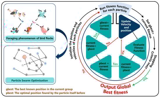
Figure 2.
Schematic diagram of the Particle Swarm Optimization algorithm.
2.5. Model Accuracy Evaluation
This study divided 1560 sampling points into a modeling set (80%, n = 1248) and a validation set (20%, n = 312), where the modeling set was used to construct the regression model and the validation set was used to evaluate the predictive performance of the model.
To assess the predictive performance of the model, four key indicators were selected: mean absolute error (MAE), root mean square error (RMSE), the coefficient of determination (R2) from the linear regression between predicted and observed values, and Lin’s concordance correlation coefficient (LCCC). Their corresponding calculation formulas are as follows:
In these equations, n represents the number of validation samples, and Pi denote the observed and predicted values at sample point , respectively. The symbols and indicate the mean values of the observed and predicted data, while r is the Pearson correlation coefficient between the two. Additionally, and represent the standard deviations of the observed and predicted values, respectively. MAE and RMSE quantify the numerical error of the predictions, where smaller values indicate higher model accuracy [35]. The R2 value primarily assesses the model’s ability to capture the trend of variation in the observed data, with higher values indicating better predictive performance [36]. LCCC, beyond measuring correlation strength, also accounts for prediction bias, providing a more comprehensive evaluation of both predictive accuracy and trend consistency [37]. An ideal predictive model should yield low MAE and RMSE values while achieving high R² and LCCC values.
3. Result and Discussion
3.1. Basic Statistics of Soil pH Content
As an initial step, descriptive statistics were calculated for soil pH in both the training and validation datasets. The results (Table 2) revealed that soil pH ranged from 4.02 to 8.50, with the maximum (Max), minimum (Min), average (AVE), and standard deviation (SD) values showing strong consistency between the two datasets. The coefficient of variation (CV) was used to assess the spatial variability of soil properties. A CV below 10% indicates weak variability, whereas a CV exceeding 100% suggests strong variability. Intermediate values signify moderate variability. According to Table 2, soil pH in the study area exhibited moderate spatial variability.
Table 2.
Descriptive statistics of soil pH at sampling points in the study area.
3.2. Explanation of the Driving Force of Spatial Heterogeneity in Soil pH
3.2.1. Pearson Correlation Analysis
To investigate the linear relationships between soil pH and environmental variables, Pearson correlation analysis was conducted (Figure 3). The results indicated that soil pH had a highly significant negative correlation with Tm (−0.432 **), LST_m (−0.424 **), E_m (−0.275 **), MRVBF (−0.207 **), and SR (−0.102 **) (p < 0.01). Additionally, it exhibited a significant positive correlation with CNBL (0.578 **), DEM (0.539 **), Hm (0.319 **), Pm (0.216 **), TU (0.144 **), TRI (0.116 **), and SCD (0.114 **). Moreover, MSAVI (0.107 **), sand (0.102 **), and GEMI (0.097 **) showed highly significant positive correlations (p < 0.01). These findings highlight that topographical, climatic, and biological factors play a crucial role in shaping the spatial distribution of soil pH in the study area.
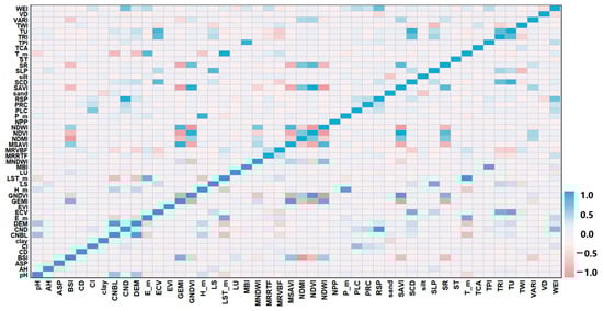
Figure 3.
Thermal map of correlation coefficients between soil pH and environmental covariates.
3.2.2. Importance Assessment of Environmental Variables Based on the RF Model
Using the Random Forest (RF) model, the importance of all environmental variables involved in the modeling process was assessed (Figure 4). The results indicated that DEM, CNBL, Tm, E_m, LST_m, and silt had the highest contributions to the model, followed by clay, Hm, MNDWI, and others. Overall, terrain attributes, climatic factors, and soil texture were identified as the most influential environmental variables affecting the spatial distribution of soil pH in the study area.
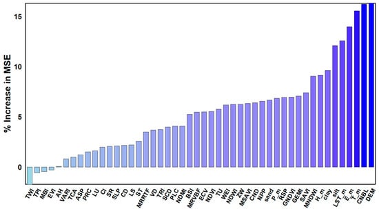
Figure 4.
Ranking of the % IncMSE values of various influencing factors in the Random Forest model.
3.2.3. SHAP Interpretation Model Results
The SHAP model is used to measure the importance of environmental variables by calculating their marginal contributions to the soil pH prediction output. Compared with the RF importance assessment, this can better explain nonlinear and interactive effects. This study uses SHAP analysis to explain the important driving factors found with the RF model, and Figure 5 and Figure 6 show a visualization of 47 environmental variables that affect soil pH. Among them, CNBL shows the highest importance, followed by DEM, LST_m, T_m, H_m, E_m, P_m, NPP, GNDVI, NDWI, MRVBF, and WEI.
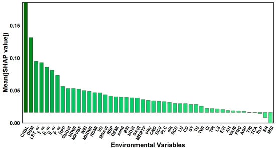
Figure 5.
Shapley values between pH and environmental variables. The overall importance of each variable is shown, with the x-axis representing the ranking of environmental variable importance and the y-axis representing the average SHAP value of each influencing factor.
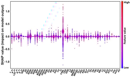
Figure 6.
Colony plot of Shapley values between pH and environmental variables. The x-axis represents the ranking of environmental variable importance, while the y-axis indicates the average SHAP value for each influencing factor. The overall importance and directional impact of each variable are visually depicted. In this figure, the SHAP value serves as a standardized index measuring the influence of each factor within the model. Red and blue dots correspond to the values of environmental variables, with SHAP > 0 indicating a positive contribution and SHAP < 0 signifying a negative impact. As the SHAP value increases, the corresponding factor has a stronger positive effect on soil pH content, whereas a decreasing SHAP value reflects a greater negative influence.
The results of the SHAP interpretation model for soil pH content in the study area highlight that topographic, biological, and climatic factors play a significant role in shaping the spatial distribution of soil pH. These environmental variables exert varying degrees of influence on soil pH variation across the region.
The combined results of the Pearson correlation analysis, RF model importance assessment, and SHAP interpretation model indicate that CNBL, DEM, LSTM, H_m, E_m, and P_m are important influencing factors of soil pH. Among the terrain factors, the Channel Network Base Level (CNBL) and Elevation (DEM) exhibit a significant correlation with the soil pH value. The CNBL and DEM data serve as crucial indicators that can intuitively mirror the undulations and variations in the terrain’s topography. These topographical characteristics, in turn, are likely to give rise to disparities in climate conditions, encompassing parameters such as temperature and precipitation. These climate variables play a pivotal role in influencing the soil pH value, as evidenced by previous research [38].
Specifically, with respect to Elevation (DEM), as the elevation increases, the atmospheric conditions change, leading to a gradual decrease in temperature. This temperature gradient has a profound impact on the activity of soil microorganisms. Soil microorganisms are key participants in the decomposition of organic matter in the soil ecosystem. A decrease in temperature can slow down their metabolic activities, thereby reducing the rate of organic matter decomposition. Since the decomposition of organic matter is intricately linked to the release and consumption of various chemical substances that affect soil pH, changes in the decomposition rate ultimately influence the soil pH content. In addition to elevation, the CNBL data are also of great significance as they can reflect the complex processes of soil erosion and sedimentation [39]. Soil erosion, which is often exacerbated by factors such as steep slopes and intense rainfall, can lead to the loss of essential soil nutrients. These nutrients are integral components that contribute to the maintenance of soil pH balance. Moreover, soil erosion can disrupt the soil structure, altering the physical and chemical properties of the soil and thus affecting the spatial distribution of soil pH. On the contrary, the sedimentation process can introduce new nutrients and organic matter into the soil. These newly added substances can interact with the existing soil components, potentially altering the soil’s chemical composition and having a direct impact on the soil pH value [40].
When considering the climatic factors, the values of the T_m, E_m, LST_m, and H_m exert significant influences on soil pH. Annual precipitation, as a key climatic variable, has a notable effect on soil acidification. Typically, an increase in annual precipitation promotes soil acidification. This occurs because precipitation acts as a leaching agent, dissolving and removing alkaline ions such as Ca2⁺ and Mg2⁺ from the soil. As these alkaline ions are leached out, the soil’s buffering capacity, which is crucial for maintaining a stable pH, is reduced. Consequently, the soil pH decreases, leading to acidification.
In regions with higher annual evaporation rates, the process of evapotranspiration is enhanced. This can result in the accumulation of salts in the soil, as water evaporates and leaves behind dissolved salts. The accumulation of salts can disrupt the soil’s chemical equilibrium, thereby affecting its acidity and alkalinity [2,41]. Mean annual humidity is closely intertwined with annual precipitation. High humidity levels are usually associated with higher precipitation amounts. The increased precipitation, as mentioned earlier, can further exacerbate the process of soil acidification by promoting the leaching of alkaline ions.
Furthermore, the mean annual ground temperature and mean annual temperature are important factors that can modulate the biological and chemical reaction rates within the soil. Higher temperatures can accelerate the decomposition of organic matter in the soil. During the decomposition process, various acidic or alkaline substances may be released. These substances can directly participate in chemical reactions that determine the soil pH, thus causing changes in the soil’s acidity or alkalinity. In essence, these climatic factors do not act in isolation but rather interact and collaborate with each other, collectively determining the spatial distribution patterns and dynamic changes of soil pH [42,43]. This complex interplay highlights the need for a comprehensive understanding of the multiple factors involved in order to accurately predict and manage soil pH in different environments.
3.3. Optimization of Variable Combinations Based on Different Environmental Variable Screening Methods
Figure 7 shows the feature selection results for pH values using the Boruta algorithm, a robust feature selection method. In the Boruta feature selection plot, green represents features identified as significant, red denotes features determined to be insignificant, and yellow indicates features still undergoing verification. The algorithm generates shadow features as a reference to evaluate the significance of actual features. In the graph, shadowMin, shadowMean, and shadowMax represent the minimum, average, and maximum Z-scores of shadow features, respectively, serving as a benchmark for real-feature importance. In accordance with the fundamental selection principle of the Boruta algorithm, features are considered significant if their impact on the importance score of pH values surpasses that of shadowMax. In the present study, the variables identified as having such a significant influence include CNBL, which is a crucial hydrological parameter related to the base elevation of the channel network within the study area and can impact water flow and sediment deposition patterns, thereby affecting soil properties including pH; DEM, which captures the topographical variations and is associated with differences in climate, water runoff, and soil formation processes that can all contribute to variations in soil pH; T_m, LST_m, H_m, E_m, and P_m, which are key climatic factors that can directly or indirectly influence soil chemical and biological processes related to pH; WEI and NDWI, which are often used to detect water bodies and can be related to soil moisture and nutrient leaching affecting pH; MRVBF, GNDVI, GEMI, VD, SAVI, NDVI, and NPP, which are biological-related factors that can impact soil organic matter content and decomposition rates, thus influencing pH; sand, MNDWI, MSAVI, NDMI, RSP, ECV, BSI, clay, ST, MRRTF, and silt.
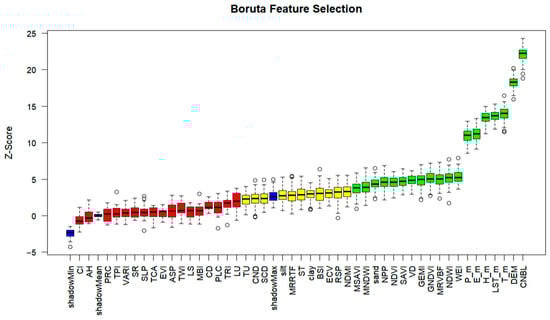
Figure 7.
Feature screening results for pH values based on the Boruta algorithm.
These identified features are classified as ’important’ and are earmarked for retention in subsequent modeling endeavors. This is because they have demonstrated a statistically significant association with the pH values within the study area. Conversely, variables whose feature importance scores fall below that of shadowMax are excluded from the modeling process, as they are considered to have a negligible or non-significant impact on the pH values and, therefore, are unlikely to contribute meaningfully to the predictive power of the model. As clearly observable in Figure 7, within the specified study area, the terrain factors CNBL and DEM play a particularly prominent role in influencing soil pH. CNBL reflects the hydrological regime within the watershed, including aspects such as the base level for water flow, which can affect the movement of solutes and the overall soil–water–nutrient balance, all of which have implications for soil pH. DEM, on the other hand, encapsulates the geomorphological characteristics of the landscape, such as slope, aspect, and elevation gradients. These topographical features can lead to variations in microclimates, water infiltration rates, and soil erosion or deposition patterns, all of which can contribute to more nuanced spatial changes in soil processes related to pH. Climatic factors follow closely in terms of their impact on soil pH.
The feature selection process culminated in the identification of a total of eight terrain factors (CNBL, DEM, ECV, MRVBF, MRRTF, RSP, VD, WEI), five climatic factors (T_m, LST_m, H_m, E_m, P_m), one soil type (ST), ten biological factors (NDWI, GNDVI, GEMI, SAVI, NDVI, NPP, MNDWI, MSAVI, NDMI, BSI), and three soil textures (clay, silt, sand). These selected features provide a comprehensive set of predictors that can be utilized in subsequent modeling to gain a more in-depth understanding of the factors governing soil pH values and to develop accurate predictive models for soil pH in the study area. This, in turn, can have significant implications for soil management, environmental monitoring, and ecological studies within the region.
In this study, the RFE algorithm and PSO algorithm were used to screen environmental variables. The Recursive Feature Elimination algorithm used an SVM as the underlying model, while the PSO algorithm used an RF as the underlying model. Both methods used ten-fold cross-validation as the model evaluation method, and the change in the RMSE was used as a reference to find the optimal feature set. By repeatedly constructing the model, the best features were selected based on the model’s feature coefficients or importance.
Figure 8 and Figure 9 show the results of screening environmental variables of soil pH based on the RFE algorithm and PSO algorithm, respectively, with the RMSE as the evaluation index. From the graph, it can be seen that as the number of feature variables increases or decreases, the RMSE shows significantly different trends, indicating that the number of environmental variables does not determine the performance of the model when constructing a prediction model. As shown in Figure 8, according to the feature selection results for soil pH in the study area based on the RFE algorithm, it can be seen that when the RMSE reaches the lowest value, the optimal number of predictive factors is 4. Therefore, this group is the selected optimal variable set. At this point, the selected set of environmental variables includes the following: one terrain factor (CNBL) and three climatic factors (P_m, LST_m, E_m). As shown in Figure 8, according to the feature screening results for soil pH in the study area based on the PSO algorithm, it can be seen that when the RMSE reaches the lowest value, the optimal number of predictive factors is 7. Therefore, this group is the selected optimal variable set. At this point, the selected set of environmental variables includes two terrain factors (CNBL, DEM) and five climatic factors (E_m, H_m, LST_m, T_m, P_m).
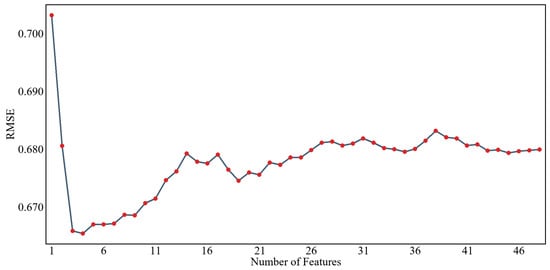
Figure 8.
Feature screening results for pH values based on the RFE algorithm.
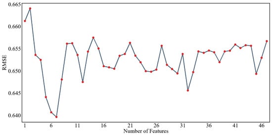
Figure 9.
Feature screening results for pH values based on the PSO algorithm.
Based on the three feature variable screening methods (the Boruta algorithm, Recursive Feature Elimination, and Particle Swarm Optimization), in combination with the principles and steps of variable screening in each method, a set of environmental variables that effectively characterize the spatial distribution of soil pH in the study area were selected through comparative selection. As shown in Table 3, the results of the screening showed that the majority of the screened variables had significant correlations with soil properties to varying degrees. Based on the selected set of effective environmental variables and the ranking of the importance of all environmental variables based on the RF model, it can be seen that when predicting soil pH, the environmental variable sets selected by the Boruta, RFE, and PSO algorithms are all located in the set with positive importance of all variables, accounting for 57.45% (27/47), 8.51% (4/47), and 14.89% (7/47), respectively.
Table 3.
Variable screening results of the Boruta, REF, and PSO algorithms.
3.4. Cross-Validation Results
The prediction results of each model were externally validated using the MAE, RMSE, R2, and LCCC, as shown in Table 4. The accuracy of the soil pH prediction model based on the RF model combined with full-variable and different-variable screening methods showed that the variable set screened using REF and PSO maintained high prediction accuracy and correlation while reducing the number of variables, and it had low prediction errors. In particular, the PSO-RF model (MAE = 0.496, RMSE = 0.641, R2 = 0.413, LCCC = 0.508) performed the best in predicting soil pH values in the study area. Next was the RFE-RF model (MAE = 0.565, RMSE = 0.662, R2 = 0.317, LCCC = 0.479). The RF model with all variables had the lowest predictive performance (MAE = 0.753, RMSE = 0.888, R2 = 0.233, LCCC = 0.237). The predictive performance of these models was in the following order: PSO-RF > RFE-RF > Boruta RF > RF. The PSO method was the best combined method for predicting soil pH in the study area because of its inclusion of the RF model, which provided advantages in reducing the number of variables and maintaining low prediction errors.
Table 4.
Cross-validation results of different interpolation methods.
The performance of the Random Forest (RF) model is significantly influenced by the selection of predictor variables. When incorporating all available variables, RF suffers from excessive noise, redundancy, and multicollinearity, which undermine model stability and predictive accuracy. Although RF is theoretically resistant to overfitting, an overabundance of irrelevant features increases uncertainty in tree pruning and weakens the contribution of key predictors, leading to performance fluctuations. Additionally, model performance is determined not solely by the presence of key variables (e.g., CNBL, DEM, T_m) but also by interactions among variables. The inclusion of redundant features can dilute the influence of critical predictors, reducing generalization ability. Moreover, the complex topography of the study area introduces additional challenges, as microtopographic heterogeneity alters the relationships between environmental variables and soil pH, affecting prediction accuracy.
Different variable selection methods influence RF performance to varying degrees. The Boruta algorithm employs strict significance screening to ensure the inclusion of essential variables but may exclude features that contribute to meaningful variable interactions, resulting in information loss and the lowest prediction accuracy among the three methods. RFE adopts a stepwise elimination strategy to refine the feature subset but is prone to local optima, potentially omitting informative variables and limiting model performance. In contrast, PSO performs a global search and combinatorial optimization, effectively identifying the optimal feature subset. Even variables with weak individual effects can enhance model performance when considered in combination, enabling PSO-RF to achieve the highest predictive accuracy.
Furthermore, RF’s inherent randomness, including bootstrapped sampling and feature selection, contributes to variability across different runs, affecting the consistency of results among different RF-based models. By leveraging intelligent swarm-based search, PSO efficiently selects the most informative variable combinations, reduces redundancy, and enhances model interpretability. As a result, the PSO-RF approach demonstrates superior efficiency in variable selection and achieves the highest prediction performance, making it a robust choice for improving soil pH modeling in complex terrains.
3.5. Spatial Distribution of Soil pH
The spatial distribution of soil pH in the study area predicted with the Boruta-RF, RFE-RF, and PSO-RF models based on the full-variable RF model and feature screening is shown in Figure 10. Overall, the spatial distribution trend of soil pH predicted by the three models in the study area is basically consistent, with most soils being acidic, showing a spatial distribution pattern where soil pH values in the eastern and northern regions are higher than those in the central, western, and southern regions. This distribution pattern may be closely related to terrain undulations and hydrological conditions.
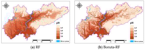
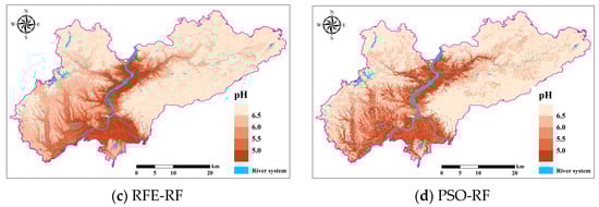
Figure 10.
Spatial distribution of pH according to four soil attribute prediction methods.
The spatial distribution of soil pH exhibits significant variation, influenced by a combination of natural and anthropogenic factors. Topographic and hydrological conditions play a crucial role in shaping pH patterns. In the eastern and northern regions, where terrain undulations are pronounced and drainage performance is relatively high, soil moisture is rapidly removed, reducing the potential for prolonged leaching of alkaline substances. This process may facilitate the accumulation of alkaline cations such as calcium (Ca2+), sodium (Na+), and potassium (K+), thereby maintaining higher pH values and approaching neutrality [44]. Furthermore, the heterogeneity in topographic relief contributes to spatial differences in hydrological conditions. Low-lying areas are more prone to water accumulation, while elevated regions exhibit enhanced drainage, potentially mitigating extreme pH variations.
In areas with significant topographic relief, the rapid movement of water limits the transport and leaching of minerals, including carbonates and calcium-containing compounds. These retained minerals may undergo chemical reactions that buffer soil acidity, thereby stabilizing soil pH at relatively neutral levels [45]. Conversely, the central, western, and southern regions, which are more influenced by adjacent water bodies, are subject to intensive hydrological leaching. This process facilitates the removal of alkaline substances while promoting the accumulation of acidic components, such as hydrogen ions (H+) and organic acids, leading to a gradual decline in soil pH [46]. Additionally, wetlands and riparian zones are typically characterized by high organic matter content and sustained moisture conditions, which enhance microbial decomposition and the subsequent production of organic acids (e.g., humic acid, oxalic acid). These acids contribute to further reductions in soil pH [47]. In contrast, in areas with more pronounced topographic variability, the distribution and decomposition of organic matter may be more spatially heterogeneous, potentially leading to lower organic acid accumulation and comparatively stable pH conditions.
Beyond natural factors, anthropogenic activities also play a critical role in shaping soil pH dynamics. Lanxi City has a registered population of 660,000. It has a well-developed industrial sector, including chemical, metal smelting, and textile industries, which may influence soil pH through the emission of acidic or alkaline aerosols. Additionally, agricultural activities are widespread in the study area, with major crops including, e.g., rice, wheat, and rapeseed and common farming practices involving nitrogen fertilizers, phosphate fertilizers, and liming. The application of nitrogen fertilizers can lead to soil acidification, whereas liming may increase soil alkalinity. These anthropogenic factors introduce additional complexity to soil pH distribution and should be considered alongside natural drivers to comprehensively understand spatial patterns.
Although the models show consistency in predicting the spatial distribution trend of soil pH, variations in prediction performance exist among different models. These differences arise from the distinct variable selection mechanisms of each model, leading to variations in the subsets of explanatory variables included in the modeling process. The ability of different models to capture key influencing factors at varying levels of detail results in discrepancies in local-scale soil pH predictions. Furthermore, the exclusion or underrepresentation of anthropogenic influence in certain models may contribute to differences in predictive performance. Therefore, incorporating human activity indicators, such as industrial emission data, fertilizer application rates, or land use patterns, could enhance model accuracy and provide a more comprehensive understanding of soil pH dynamics.
4. Conclusions
- (1)
- The prediction accuracy of the RF model using the Boruta, Recursive Feature Elimination (RFE), and Particle Swarm Optimization (PSO) feature selection methods is better than that of the RF model with all variables. Therefore, it is necessary to screen for environmental variables before establishing a machine learning model, and this can improve the accuracy of the model. The order of prediction accuracy for the four models is PSO-RF > RFE-RF > Boruta-RF > RF.
- (2)
- The Pearson correlation analysis, RF model importance assessment, and SHAP interpretation model all indicate that CNBL, DEM, T_m, E_m, LST_m, and H_m are key factors affecting soil pH. These variables are closely related to the characteristics of terrain changes, microclimatic conditions, and hydrological processes, which collectively affect the spatial distribution of pH.
- (3)
- The spatial distribution trend of soil pH in the four models is basically consistent, showing an overall acidic characteristic. The soil pH values in the eastern and northern regions are relatively high, while the pH values in the central, western, and southern regions are lower. This distribution pattern is closely related to terrain undulations and hydrological conditions. The terrain in the eastern and northern regions is undulating, with good water drainage and accumulation of alkaline substances. The soil pH tends to be more neutral, while the central, western, and southern regions have more water bodies. Due to excessive water content, acidic substances accumulate, resulting in lower soil pH values and exhibiting acidic characteristics.
Author Contributions
Conceptualization, H.H. and Y.L. (Yaolin Liu); Methodology, H.H. and Y.L. (Yanfang Liu); Software, Z.T.; Validation, Y.L. (Yaolin Liu) and Z.R.; Formal Analysis, Z.T. and Y.L. (Yanfang Liu); Investigation, H.H.; Resources, Z.R. and Y.L. (Yanfang Liu). Data Curation, Z.R. and Z.T.; Writing—Original Draft, H.H.; Writing—Review and Editing, Y.X. and Z.T.; Visualization, Y.X. and Y.L. (Yanfang Liu); Supervision, Y.L. (Yanfang Liu) and Z.T.; Funding acquisition, Y.L. (Yaolin Liu). All authors have read and agreed to the published version of the manuscript.
Funding
The authors acknowledge the support of the project “the Key Program of National Natural Science Foundation of China” (42230107), the “National Natural Science Foundation of China”(42471454), and the ”Strategic Science and Technology Talent Cultivation Special Project of Hubei province” (2024DJA012).
Institutional Review Board Statement
Not applicable.
Informed Consent Statement
Not applicable.
Data Availability Statement
The original contributions presented in this study are included in this article; further inquiries can be directed to the corresponding author.
Conflicts of Interest
The authors declare no conflicts of interest.
References
- Huang, J.; Wong, V.N.L.; Triantafilis, J. Mapping soil salinity and pH across an estuarine and alluvial plain using electromagnetic and digital elevation model data. Soil Use Manag. 2014, 30, 394–402. [Google Scholar]
- Lu, Q.; Tian, S.; Wei, L. Digital mapping of soil pH and carbonates at the European scale using environmental variables and machine learning. Sci. Total Environ. 2023, 856, 159171. [Google Scholar]
- Forkuor, G.; Hounkpatin, O.K.L.; Welp, G.; Thiel, M. High Resolution Mapping of Soil Properties Using Remote Sensing Variables in South-Western Burkina Faso: A Comparison of Machine Learning and Multiple Linear Regression Models. PLoS ONE 2017, 12, e0170478. [Google Scholar]
- Vandana, N.; Suresh, G.J.; Mitran, T.; Mahadevappa, S.G. Digital Mapping of Soil pH and Electrical Conductivity Using Geostatistics and Machine Learning. Int. J. Environ. Clim. Change 2024, 14, 273–286. [Google Scholar]
- Rossiter, D.G.; Poggio, L.; Beaudette, D.; Libohova, Z. How well does digital soil mapping represent soil geography? An investigation from the USA. Soil 2022, 8, 559–586. [Google Scholar]
- Öztürk, M.; Kiliç, M.; Günal, H. Digital Mapping of Soil pH and Electrical Conductivity: A Comparative Analysis of Kriging and Machine Learning Approaches. MAS J. Appl. Sci. 2024, 9, 1168–1185. [Google Scholar]
- Zhao, X.; He, C.; Liu, W.S.; Liu, W.X.; Liu, Q.Y.; Bai, W.; Li, L.J.; Lal, R.; Zhang, H.L. Responses of soil pH to no-till and the factors affecting it: A global meta-analysis. Glob. Change Biol. 2022, 28, 154–166. [Google Scholar]
- Demas, G.P.; Rabenhorst, M.C. Factors of subaqueous soil formation: A system of quantitative pedology for submersed environments. Geoderma 2001, 102, 189–204. [Google Scholar]
- McBratney, A.B.; Odeh, I.O.A.; Bishop, T.F.A.; Dunbar, M.S.; Shatar, T.M. An overview of pedometric techniques for use in soil survey. Geoderma 2000, 97, 293–327. [Google Scholar]
- Ma, Y.; Minasny, B.; Malone, B.P.; Mcbratney, A.B. Pedology and digital soil mapping (DSM). Eur. J. Soil Sci. 2019, 70, 216–235. [Google Scholar] [CrossRef]
- Tanasă, I.C.; Niculită, M.; Roșca, B.; Pîrnău, R. Pedometric techniques in spatialisation of soil properties for agricultural land evaluation. Bull. Univ. Agric. Sci. Vet. Med. Cluj-Napoca Agric. 2010, 67, 274–278. [Google Scholar]
- Ballabio, C. Spatial prediction of soil properties in temperate mountain regions using support vector regression. Geoderma 2009, 151, 338–350. [Google Scholar]
- Kovačević, M.; Bajat, B.; Gajić, B. Soil type classification and estimation of soil properties using support vector machines. Geoderma 2010, 154, 340–347. [Google Scholar] [CrossRef]
- Dharumarajan, S.; Hegde, R.; Singh, S.K. Spatial prediction of major soil properties using Random Forest techniques-A case study in semi-arid tropics of South India. Geoderma Reg. 2017, 10, 154–162. [Google Scholar] [CrossRef]
- da Silva Chagas, C.; de Carvalho Junior, W.; Bhering, S.B.; Calderano Filho, B. Spatial prediction of soil surface texture in a semiarid region using random forest and multiple linear regressions. Catena 2016, 139, 232–240. [Google Scholar] [CrossRef]
- Kohavi, R.; John, G.H. Wrappers for feature subset selection. Artif. Intell. 1997, 97, 273–324. [Google Scholar]
- Nilsson, R.; Pena, J.M.; Björkegren, J.; Tegnér, J. Consistent feature selection for pattern recognition in polynomial time. J. Mach. Learn. Res. 2007, 8, 589–612. [Google Scholar]
- Chen, Y.W.; Lin, C.J. Combining SVMs with various feature selection strategies. Feature Extr. Found. Appl. 2006, 207, 315–324. [Google Scholar]
- Kursa, M.B.; Jankowski, A.; Rudnicki, W.R. Boruta–a system for feature selection. Fundam. Informaticae 2010, 101, 271–285. [Google Scholar]
- Cools, N.; Delanote, V.; Scheldeman, X.; Quataert, P.; De Vos, B.; Roskams, P. Quality assurance and quality control in forest soil analyses: A comparison between European soil laboratories. Accredit. Qual. Assur. 2004, 9, 688–694. [Google Scholar]
- McBratney, A.B.; Santos, M.L.M.; Minasny, B. On digital soil mapping. Geoderma 2003, 117, 3–52. [Google Scholar] [CrossRef]
- Zeraatpisheh, M.; Ayoubi, S.; Jafari, A.; Tajik, S.; Finke, P. Digital mapping of soil properties using multiple machine learning in a semi-arid region, central Iran. Geoderma 2019, 338, 445–452. [Google Scholar] [CrossRef]
- Mousavi, A.; Karimi, A.; Maleki, S.; Safari, T.; Taghizadeh-Mehrjardi, R. Digital mapping of selected soil properties using machine learning and geostatistical techniques in Mashhad plain, northeastern Iran. Environ. Earth Sci. 2023, 82, 234. [Google Scholar]
- Lundberg, S. A unified approach to interpreting model predictions. arXiv 2017, arXiv:1705.07874. [Google Scholar]
- Wadoux, A.M.J.C.; Saby, N.P.A.; Martin, M.P. Shapley values reveal the drivers of soil organic carbon stock prediction. Soil 2023, 9, 21–38. [Google Scholar] [CrossRef]
- Rossel, R.A.V.; Behrens, T. Using data mining to model and interpret soil diffuse reflectance spectra. Geoderma 2010, 158, 46–54. [Google Scholar] [CrossRef]
- Vohland, M.; Emmerling, C. Determination of total soil organic C and hot water-extractable C from VIS-NIR soil reflectance with partial least squares regression and spectral feature selection techniques. Eur. J. Soil Sci. 2011, 62, 598–606. [Google Scholar]
- Liess, M.; Hitziger, M.; Huwe, B. The Sloping Mire Soil-Landscape of Southern Ecuador: Influence of Predictor Resolution and Model Tuning on Random Forest Predictions. Appl. Environ. Soil Sci. 2014, 2014, 57–66. [Google Scholar] [CrossRef]
- Wang, X.; Ding, J.; Han, L.; Tan, J.; Ge, X. Enhancing soil particle content prediction accuracy: Advanced hyperspectral analysis and machine learning models. J. Soils Sediments Prot. Risk Assess. Remediat. 2024, 24, 3443–3458. [Google Scholar]
- Zhou, Q.; Ding, J.; Ge, X.; Li, K.; Zhang, Z.; Gu, Y. Estimation of soil organic matter in the Ogan-Kuqa River Oasis, Northwest China, based on visible and near-infrared spectroscopy and machine learning. J. Arid Land 2023, 15, 191–204. [Google Scholar] [CrossRef]
- Arrouays, D.; Grundy, M.G.; Hartemink, A.E.; Hempel, J.W.; Heuvelink, G.B.; Hong, S.Y.; Lagacherie, P.; Lelyk, G.; McBratney, A.B.; McKenzie, N.J.; et al. GlobalSoilMap: Toward a Fine-Resolution Global Grid of Soil Properties. Adv. Agron. 2014, 125, 93–134. [Google Scholar]
- Xue, B.; Zhang, M.; Browne, W.N. Particle swarm optimization for feature selection in classification: A multi-objective approach. IEEE Trans. Cybern. 2013, 43, 1656–1671. [Google Scholar] [PubMed]
- Niu, D.X.; Guo, Y.C. An Improved PSO for Parameter Determination and Feature Selection of SVR and its Application in STLF. J. Mult.-Valued Log. Soft Comput. 2010, 16, 567. [Google Scholar]
- Zhang, Y.; Gong, D.W.; Cheng, J. Multi-Objective Particle Swarm Optimization Approach for Cost-Based Feature Selection in Classification. IEEE/ACM Trans. Comput. Biol. Bioinform. 2017, 14, 64–75. [Google Scholar] [CrossRef] [PubMed]
- Mondal, A.; Khare, D.; Kundu, S.; Mondal, S.; Mukherjee, S.; Mukhopadhyay, A. Spatial soil organic carbon (SOC) prediction by regression kriging using remote sensing data. Egypt. J. Remote Sens. Space Sci. 2017, 20, 61–70. [Google Scholar] [CrossRef]
- Chen, S.; Mulder, V.L.; Heuvelink, G.B.M.; Poggio, L.; Caubet, M.; Dobarco, M.R.; Walter, C.; Arrouays, D. Model averaging for mapping topsoil organic carbon in France. Geoderma 2020, 366, 114237. [Google Scholar]
- Lamichhane, S.; Kumar, L.; Wilson, B. Digital soil mapping algorithms and covariates for soil organic carbon mapping and their implications: A review. Geoderma 2019, 352, 395–413. [Google Scholar]
- Gardi, C.; Yigini, Y. Continuous mapping of soil pH using digital soil mapping approach in Europe. Eurasian J. Soil Sci. 2012, 1, 64–68. [Google Scholar]
- Xia, Y.; McSweeney, K.; Wander, M.M. Digital mapping of agricultural soil organic carbon using soil forming factors: A review of current efforts at the regional and national scales. Front. Soil Sci. 2022, 2, 890437. [Google Scholar] [CrossRef]
- Zhou, Y.; Zhao, X.; Guo, X.; Li, Y. Mapping of soil organic carbon using machine learning models: Combination of optical and radar remote sensing data. Soil Sci. Soc. Am. J. 2022, 86, 293–310. [Google Scholar] [CrossRef]
- Zhang, J.; Schmidt, M.G.; Heung, B.; Bulmer, C.E.; Knudby, A. Using an ensemble learning approach in digital soil mapping of soil pH for the Thompson-Okanagan region of British Columbia. Can. J. Soil Sci. 2022, 102, 579–596. [Google Scholar]
- Liu, Y.; Han, X.; Zhu, Y.; Li, H.; Qian, Y.; Wang, K.; Ye, M. Spatial mapping and driving factor Identification for salt-affected soils at continental scale using Machine learning methods. J. Hydrol. 2024, 639, 131589. [Google Scholar] [CrossRef]
- Esmaeilizad, A.; Shokri, R.; Davatgar, N.; Dolatabad, H.K. Exploring the driving forces and digital mapping of soil biological properties in semi-arid regions. Comput. Electron. Agric. 2024, 220, 108831. [Google Scholar] [CrossRef]
- Zhao, C.; Li, P.; Yan, Z.; Zhang, C.; Meng, Y.; Zhang, G. Effects of landscape pattern on water quality at multi-spatial scales in Wuding River Basin, China. Environ. Sci. Pollut. Res. 2024, 31, 19699–19714. [Google Scholar]
- Chen, S.; Arrouays, D.; Mulder, V.L.; Poggio, L.; Minasny, B.; Roudier, P.; Libohova, Z.; Lagacherie, P.; Shi, Z.; Hannam, J.; et al. Digital mapping of GlobalSoilMap soil properties at a broad scale: A review. Geoderma 2022, 409, 115567. [Google Scholar]
- Asgari, N.; Ayoubi, S.; Demattê, J.A.M.; Jafari, A.; Safanelli, J.L.; Da Silveira, A.F. Digital mapping of soil drainage using remote sensing, DEM and soil color in a semiarid region of Central Iran. Geoderma Reg. 2020, 22, e00302. [Google Scholar]
- Costa, E.M.; Samuel-Rosa, A.; Anjos, L.H.C. Digital elevation model quality on digital soil mapping prediction accuracy. Ciência. Agrotecnol. 2018, 42, 608–622. [Google Scholar]
Disclaimer/Publisher’s Note: The statements, opinions and data contained in all publications are solely those of the individual author(s) and contributor(s) and not of MDPI and/or the editor(s). MDPI and/or the editor(s) disclaim responsibility for any injury to people or property resulting from any ideas, methods, instructions or products referred to in the content. |
© 2025 by the authors. Licensee MDPI, Basel, Switzerland. This article is an open access article distributed under the terms and conditions of the Creative Commons Attribution (CC BY) license (https://creativecommons.org/licenses/by/4.0/).