Short-Term Residential Load Forecasting Based on the Fusion of Customer Load Uncertainty Feature Extraction and Meteorological Factors

Abstract

With the proliferation of distributed energy resources, advanced metering infrastructure, and advanced communication technologies, the grid is transforming into a flexible, intelligent, and collaborative system. Short-term electric load forecasting for individual residential customers is playing an increasingly important role in the operation and planning of the future grid. Predicting the electrical load of individual households is more challenging with higher uncertainty and volatility at the household level compared to the total electrical load at the feeder and regional levels. The previous research results show that the accuracy of forecasting using machine learning and a single deep learning model is far from adequate and there is still room for improvement.

1. Introduction

Electricity, the most important energy source available today, is essential to the security and stability of urban growth. With the advent of the smart era, traditional power grids are evolving into smart grids. The goal of smart grids is to improve energy utilization and reduce the consumption of non-renewable energy. In smart grids, one of the effective ways to improve renewable energy utilization is to reduce peak and valley and dispatch electricity in a reasonable manner. The percentage of residential electricity consumption in end-use energy consumption is rising as a result of the economy’s quick development and the development of smart grid technology. Power providers can develop reasonable demand response strategies, encourage residents to modify their innate electricity consumption patterns, lower customers’ electricity costs, and accomplish peak and valley reduction goals with the aid of an accurate residential electricity load forecast.

Power load forecasting in smart grids guarantees the safe, reliable, and cost-effective operation of power systems. Traditional load forecasting focuses on regional, system-level, feeder-level, or entire buildings. With the widespread adoption of smart meters, which allow high-frequency sampling, a large amount of high-frequency single-user electricity data is collected, making user-level load forecasting possible [1]. Smart meter data provide important information such as load profiles and individual consumption habits, which can be used to improve the accuracy of both individual and overall load forecasts. Accurate short-term load forecasting (STLF) can effectively support Home Energy Management Systems (HEMSs) [2]. Additionally, load forecasting enables power companies to determine effective electricity pricing structures and implement more rational demand response strategies, thereby reducing operational costs [3]. In order to improve energy efficiency, integrate renewable energy, lower carbon emissions, maintain grid stability, and reap economic and social benefits, user load forecasting is a crucial tool for advancing energy sustainability.

However, because users’ electricity consumption behavior exhibits high randomness and uncertainty, forecasting individual user behavior is more challenging than system-level aggregated power load curves, as the timing of usage activities introduces further randomness and noise. Compared to traditional load forecasting problems, residential load forecasting presents unique challenges. For instance, the load scale of substations or buses is relatively large and does not change within a short period. Load curves for commercial and industrial users often exhibit typical peak–valley patterns, which aid accurate load prediction. In contrast, user behavior in residential settings has its specific characteristics: electricity consumption tends to vary periodically with work, rest, and leisure time cycles. Additionally, usage behavior is easily influenced by external stimuli; for example, when temperature and humidity change, users may activate equipment to control these conditions, which ultimately reflects energy consumption.

In the field of power load forecasting, many researchers have conducted extensive studies, applying statistical and machine learning algorithms such as the Autoregressive Integrated Moving Average (ARIMA) [4] and Gaussian Process (GP) [5] to the forecasting tasks, primarily for system-level load forecasting. However, for household load forecasting, the data’s instability and user behavior uncertainty often limit these models’ effectiveness. Since single-user load data are typically a long, high-frequency sequence, previous studies [6] have identified residential power load as a combination of periodic, uncertain, and noisy data. Periodic data can often be predicted using statistical and traditional machine learning methods, while uncertainty introduces complex nonlinear patterns that are challenging for these methods to handle. With the rapid development of computing power, the ability to utilize deep learning methods has become critical in the rapidly evolving energy industry [7]. It presents a promising solution for such data. Its multilayered nonlinear structure allows it to capture complex feature abstractions and nonlinear mappings. In recent years, deep learning has made significant advances in fields such as image processing and speech recognition, leading many researchers to apply it to load forecasting tasks [8].

In summary, the following problems still exist in current deep learning-based models for short-term household electricity load forecasting:

(1)

The acquisition of user load is usually a large number of long sequences with high frequency, great randomness, and uncertainty, which still requires data preprocessing techniques for feature extraction before being input to the model.

(2)

In user-level load prediction tasks, data uncertainty-awareness enhancement is required in building deep learning models.

(3)

Most scholars compose additional features and load data simultaneously as input vectors for model training, but, in the field of deep learning, it is introduced that features can be learned individually by independent networks and then adapted to downstream prediction tasks by feature fusion.

To address the above problems, this paper proposes segmenting long sequences into multiple subsequences, aligning the data points in these subsequences relative to time for use as input vectors for the neural network, and extracting baselines from these subsequences. The proposed model first utilizes a CNN in the encoder to perform local feature extraction on the input subsequences, followed by an input attention mechanism (IAM) for weight allocation. The weighted vectors are then sequentially fed into LSTM for learning uncertainty features, yielding a power load feature vector. Since this changes the input data dimensions, causing the model to lack user power load context information, an autoregressive component is introduced for information compensation. To mitigate overfitting and enhance load data features, a separate CNN is introduced to learn local features of meteorological factors such as temperature, humidity, and dew point, resulting in a meteorological feature vector. The power load and meteorological feature vectors are then fused in a residual connected fusion module at the same time step to create a combined vector. Finally, another LSTM predicts the fused vector, yielding a nonlinear prediction value, which is added to the output of the autoregressive component for the final forecast. In summary, the main contributions of this paper are as follows.

(1)

A nonlinear relationship extraction method for customer electric load is proposed, combining subsequence partitioning and a CNN-IAM-LSTM module for feature extraction to reduce noise and capture deep load features.

(2)

Meteorological data are integrated using a first-order difference and CNN-based feature extraction network for local meteorological feature analysis.

(3)

A multifactor fusion sub-network is developed, utilizing residual connections and layer normalization to align and integrate electric load and meteorological features, enhancing model performance.

(4)

A fused multi-stage LSTM model is designed, combining feature extraction, multi-feature fusion, and prediction networks to improve user-level nonlinear capability and forecasting accuracy.

The remainder of this paper is organized as follows: Section 2 introduces the proposed model and provides a brief overview of its components. Section 3 describes the UMASS dataset and the parameter settings for model training and prediction, and discusses the prediction results and error analysis of the proposed model on three user datasets. Section 4 presents the conclusions.

2. Related Work

In the field of power load forecasting, many researchers have introduced deep learning into short-term load forecasting tasks, especially using Recurrent Neural Networks (RNNs) and temporal convolution networks (TCNs), and then used feature enhancement and other methods for optimization.

RNNs have become one of the most frequently used deep learning methods for short-term load forecasting in recent years. For instance, in reference [9], an RNN-based forecasting framework is employed for power load prediction. Compared to traditional statistical learning algorithms, RNN-based forecasting models offer significant performance improvements. By transmitting information across multiple time steps within neurons, RNNs have the theoretical capacity to leverage temporal correlations and long historical sequences in time series. However, traditional RNNs suffer from inherent issues of gradient explosion and vanishing gradients during training. Long short-term memory (LSTM) networks address the “memory problem” in RNNs by introducing gating mechanisms within the RNN neurons. The LSTM structure includes a memory cell, enabling it to retain important states from previous steps. Additionally, LSTM employs a forget gate to discard irrelevant features and reset the memory cell. As demonstrated in references [10,11], LSTM outperforms backpropagation (BP) networks and standard RNNs in power load forecasting, as it can accurately capture long- and short-term dependencies within the load data, achieving superior prediction results. In reference [12], researchers apply LSTM load forecasting at the user level, and a comprehensive comparison with LSTM predictions at the aggregated level reveals the feasibility of using LSTM for user-level predictions. The Gated Recurrent Unit (GRU), proposed by Cho in 2014 [13], is a variant of LSTM designed to address the challenge of high parameterization in LSTM that can impede convergence. Unlike LSTM, the GRU combines the input and forget gates into a single-update gate structure, reducing the number of parameters and enabling faster convergence during training. In reference [14], the GRU is used for load forecasting at the aggregate user level, where it outperforms traditional LSTM in terms of performance. At the individual user level, reference [15] evaluates LSTM, GRU, and RNN on user load data with a resolution of one minute, concluding that LSTM performs best on this dataset. Given that RNNs are designed to learn data based on time steps, some researchers have also applied bidirectional recurrent networks for load forecasting. For example, reference [16] uses a bidirectional RNN (Bi-RNN), reference [17] uses bidirectional LSTM (Bi-LSTM), and reference [18] uses a bidirectional GRU (Bi-GRU). These RNN models learn both forward and backward time step contexts in the power load time series, resulting in models with enhanced robustness; however, this also increases the number of learnable parameters, potentially reducing performance. Currently, in short-term load forecasting at the user level, models based on RNNs and their variants, LSTM and GRU, demonstrate better performance than machine learning models and conventional BP neural networks. However, they still struggle with accurate prediction of load peaks and valleys, indicating that precision remains suboptimal [19].

To enhance the predictive capability of RNN-based models in short-term electricity load forecasting, researchers have made improvements in various aspects of the RNN model. One primary direction of these improvements involves data preprocessing and feature enhancement for RNN model inputs. In reference [11], data processing techniques were used to augment LSTM performance by preprocessing input power data with an autocorrelation plot to extract hidden features before feeding it into the LSTM network for load prediction. Similarly, references [20,21] have developed deep learning models using the same approach. Reference [22] introduces a CNN-LSTM model for power forecasting, which achieved the lowest error rate compared to other baseline models due to its ability to learn both spatial and temporal features. Reference [23] proposed a VMD-based two-stage decomposition and reconstruction feature processing method, where the power load is decomposed by VMD, and input vectors of temperature, humidity, and wind speed are reconstructed, which achieves effective results when integrated with an LSTM-based predictive model. Some researchers have also employed autoencoders (AEs) for load forecasting. AEs essentially split neural networks into two parts: an encoder to extract features from data and output an intermediate vector, and a decoder to decode the intermediate vector, producing outputs based on the downstream task. In reference [24], researchers used AEs for feature extraction; after clustering similar customers, a CNN-based AE was used for dimensionality reduction, followed by LSTM to create a forecast in the encoded latent space for each cluster, which is then decoded to yield the final prediction. Similarly, reference [25] utilizes an autoencoder to address LSTM’s difficulty in capturing temporal dependencies across sequences. First, spatial features are extracted with convolutional layers and then fed into LSTM-AE to generate encoded sequences, which are finally used as feature vectors that are input to a fully connected layer for load forecasting. In reference [26], researchers compared various neural network architectures, including conventional neural networks, fully connected AE networks, RNNs, and LSTMs, concluding that AE-integrated networks form the best deep architecture, outperforming traditional models like weighted moving averages, linear regression, regression trees, SVR, and MLP.

Furthermore, TCNs, an essential deep learning technique, have demonstrated notable efficacy in short-term load forecasting, especially when working with data that contains weather and calendar information [27]. Unlike conventional RNNs, which rely on recursive structures, TCNs can efficiently capture long-range dependencies in time-series data through causal and dilated convolutions. Meanwhile, in reference [28], transformer-based models have also shown strong performance in the field of electricity load forecasting. Complex relationships between various time steps are captured by the transformer model through the use of the self-attention mechanism, which is particularly important for comprehending and forecasting changes in electricity load.

For feature enhancement, many scholars have noticed that standard RNN models treat input vectors uniformly, ignoring the varying impact of different inputs on prediction performance. By incorporating an attention mechanism (AM), input vectors or features to the RNN can be weighted to enhance key time steps or features [29]. AM has been successfully applied to image processing, natural language processing (NLP), and time-series tasks. Given that load forecasting is inherently a time-series prediction task, applying an AM to calculate the importance of load forecasting features is feasible. Reference [30] proposed an attention-based bidirectional LSTM (Attention-BiLSTM) network to accurately predict short-term power loads, addressing the limitations of traditional load forecasting methods in handling large-scale nonlinear time-series data. Likewise, in reference [19], an AM was incorporated into an RNN with residual connections to calculate the importance of input features, demonstrating that the attention-enhanced model significantly improves robustness and generalization compared to other models. In reference [31], a dual-stage attention time-series prediction model, DARNN, was proposed; it consists of an encoder with input attention to extract and weight multiple influential factors, and a decoder with a temporal attention module to decode predictions. Performance testing on multiple datasets showed that the DARNN significantly outperforms various attention-based RNN models.

Although deep learning has achieved significant progress in system-level and feeder-level load forecasting, user-level load forecasting still presents major challenges. As mentioned previously, the inherent uncertainty in user behavior data often leads to model overfitting and decreased generalizability. One effective solution is to establish a data baseline with regular patterns by processing this type of data to extract nonlinear relationships within the power load time series. For example, reference [32] transforms the power load time series into a three-dimensional hourly load cube—day, hour, and week—using a CNN for feature extraction of nonlinear relationships. Another approach is to introduce additional indicator data, such as weather factors, for feature enhancement. In reference [33], the authors compared LSTM models with and without meteorological factors, concluding that incorporating external data generally improves prediction performance. Additionally, when the input time series is too long, LSTM or GRU networks with gated memory structures may still experience issues with memory retention.

In summary, current deep learning-based short-term household electricity load forecasting models still face challenges related to the randomness and uncertainty of household electricity loads, which lead to low short-term prediction accuracy. This paper proposes a method for extracting nonlinear relationships in user electricity loads based on subsequence segmentation and CNN-IAM-LSTM. This method reduces the impact of random walk behaviors and noise interference caused by user activities, enabling the extraction of deep features of household electricity loads and improving short-term prediction accuracy.

3. Model

3.1. Problem Description

We intend to achieve a high-accuracy short-term forecast of household short-term power load based on household electricity consumption and external characteristic data, such as meteorological data. The specific definition of the problem is as follows: given a household electricity consumption time series $X=(x_1,x_2,\cdots ,x_T)$ over the past $T$ time steps, where $x_t$ denotes the consumption readings within period $t$, and a meteorological time series $Q=(q_1,q_2,\cdots ,q_m)$ composed of $m$ meteorological factors reported locally, where $q_i=(q_{i,1},q_{i,2},\cdots ,q_{i,T})$, $i\in (1,m)$ represents the time series of readings for the $i$-th meteorological factor over the past $T$ time steps. The aim of the model is to learn a nonlinear model $F(X,Q)$ to forecast household electricity consumption $Ŷ$ for the next time steps.

3.2. Model Construction

To address the challenges in short-term load forecasting—characterized by high uncertainty, numerous and random user behavior factors, and the strong generalization needed for long-sequence data—this paper proposes a short-term household electricity load forecasting model based on uncertainty feature extraction of user load and the integration of meteorological factors. The proposed model is composed of four main parts: user electricity load data subsequence partitioning and feature extraction, meteorological data feature extraction, multi-feature fusion, and prediction. In the electricity data subsequence partitioning and feature extraction stage, the long sequence is divided into multiple subsequences, and feature learning is performed using a CNN-IAM-LSTM-based neural network to obtain multiple local feature vectors. For meteorological data feature extraction, local features are obtained using a combination of first-order differencing and a CNN. The multi-feature fusion network utilizes a residual connection network to merge feature vectors from electricity data and meteorological factors. The prediction layer, composed of an independent LSTM, learns from the fused feature vectors output by the fusion layer and produces nonlinear forecast data. The final prediction result is obtained by adding this output to the autoregressive information compensation. The model structure is illustrated in Figure 1. In the remainder of this section, we briefly introduce the convolutional neural network (CNN), the long short-term memory (LSTM) network, the input attention mechanism, and the residual connection mechanism.

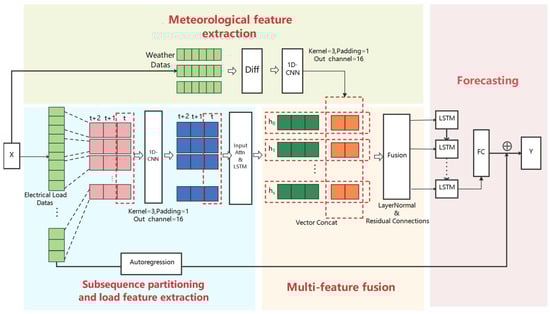
Figure 1. Model organization structure.

3.2.1. User Load Subsequence Partitioning and Local Feature Extraction

Subsequence Partitioning and CNN Feature Extraction

To further analyze the uncertainty in users’ electricity consumption, the power load sequence over the past $T$ hours is divided into subsequences, where the length of each subsequence is $L$ and the number of subsequences is $N$, so $T=L\ast N$. The division of $L$ typically takes into account human daily routines and activity cycles to maintain temporal correlations between each subsequence, represented as $X=\left(s_1,s_2,\dots ,s_N\right)$, where $S_i={(S_{i,1},S_{i,2},\cdots ,S_{i,L})}^T,i\in (1,N)$. The optimal subsequence length is determined experimentally. Local features are extracted using a convolutional neural network (CNN) without pooling layers. CNN, proposed by Lecun Y et al. in 1998, is widely applied in various deep learning fields, including image and speech recognition [34]. Reference [35] demonstrates that a 1D-CNN is effective in extracting temporal feature information from time series. CNN extracts local features through local connections, weight sharing, and spatial pooling, which enhances its capacity for abstract representation. Its main structure comprises convolutional layers, pooling layers, and fully connected layers [36]. The main formula for the CNN is shown in Equation (1):

$$y_i^k=f(y^{k-1}\ast w_i^k+b_i^k)$$

(1)

where $y^{k-1}$ represents the input of the $k$-th convolutional layer, $\ast$ denotes the convolution operation, $w_i^k$ is the weight of the $i$-th filter in the $k$-th convolutional layer, and $b_i^k$ is the bias term for the $k$-th convolutional layer. By applying the CNN convolution operation in Equation (1) to the input subsequence, the output sequence $Ŝ=({ŝ}_1,{ŝ}_2,\cdots ,{ŝ}_k)$ is obtained, where $k$ is the number of output channels.

Input Attention Weighting

The input attention mechanism (IAM) employs a deterministic attention model, namely a multilayer perceptron model. IAM applies attention to the input layer, assigning different weights to the model’s inputs, thereby significantly reducing the number of learnable parameters. This is because IAM does not require the typical encoder–decoder network used in existing attention mechanisms (Figure 2).

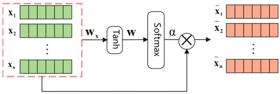
Figure 2. Input attention.

Input attention weights are calculated for multiple feature time-series vectors after local feature extraction. The input attention weight for the $j$-th feature sequence is computed as follows:

$$e_j=V_{in}^T\tanh (W_{in}{s}_j+b_{in})+b_{in}^{\prime }$$

(2)

$${\alpha }_j={\displaystyle \frac{exp\left(e_j\right)}{{\sum }_{j=1}^{n}exp\left(e_j\right)}}$$

(3)

where $V_{in}^T$, $W_{in}$, $b_{in}$, and $b_{in}^{\prime }$ are learnable parameters, and ${\alpha }_j$ is the input weight for the $j$-th feature sequence. Then, the input attention-weighted matrix for all local features can be represented as $\overline{S}=({\alpha }_1{\mathrm{ŝ}}_1,{\alpha }_2{\mathrm{ŝ}}_2,\cdots ,{\alpha }_k{\mathrm{ŝ}}_k)$, with the weighted input vector at time $t$ denoted as ${\overline{S}}_t={({\alpha }_1{\mathrm{ŝ}}_{1,t},{\alpha }_2{\mathrm{ŝ}}_{2,t},\cdots ,{\alpha }_k{\mathrm{ŝ}}_{k,t})}^T$.

LSTM Time-Series Feature Extraction

Compared with traditional RNNs, which have only a single hidden state, LSTM introduces the concept of a cell state, accounting for temporal correlations embedded in long-term states. The cell structure of the LSTM is shown in the Figure 3.

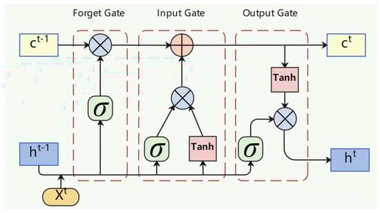
Figure 3. LSTM neuron structure.

LSTM is based on recurrent neural network by adding input gates, forget gates, and output gates to control the input and output of the information flow and the state of the cell, respectively, to achieve the update of the control information on the cell state. Calculating the output of an LSTM cell requires the calculation of the cell state at the input gate, the forget gate, and the output gate for the current input and the previous moment, respectively, and the LSTM neural cell at moment $t$ is calculated as follows:

$$\left\{\begin{array}{c}{i}_t=\sigma (W_i{x}_i+U_i{h}_{i-1}+V_i{c}_{i-1}+b_i)\\ f_t=\sigma (W_f{x}_t+U_f{h}_{t-1}+V_f{c}_{t-1}+b_f)\\ {ĉ}_t=W_c{x}_t+U_c{h}_{t-1}+b_c\\ c_t=f_t{c}_{t-1}+i_t\tanh (W_c{x}_t+U_c{h}_{t-1}+b_c)\\ o_t=\sigma (W_o{x}_t+U_o{h}_{t-1}+V_o{c}_{t-1}+b_o)\\ h_t=o_t\tanh \left(c_t\right)\end{array}\right.$$

(4)

where $c_t$ is the cell state of the memory cell at time $t$; $c_{t-1}$ denotes the cell state at the previous moment; ${ĉ}_t$ denotes the candidate state of the input; $h_t$ is all the outputs of the LSTM unit at time $t$; $W$, $U$, $V$, $b$ are the matrices of the coefficients and the vectors of the biases, respectively; $\sigma$ is the activation function Sigmoid; $x_t$ is the input at time $t$; $i_t$, $f_t$, $o_t$ are the inputs at time t and the outputs of the input, forget, and output gates at time t, respectively. The LSTM neural network in the encoder has a multilayer network structure, and each layer consists of multiple neuronal cells, whose hidden state $h_t$ at moment $t$ can be calculated by the formula:

$$h_t=f_e(h_{t-1},{\overline{S}}_t)$$

(5)

where $f_e$ is the LSTM network, and $h_{t-1}$ is the output of the LSTM at the previous moment. After LSTM layer coding, $L$ electrical load codes $H=(h_1,h_2,\cdots ,h_l)$ are obtained.

Autoregressive Information Compensation

By subsequence partitioning and feature extraction of the customer load, we extracted the uncertainty features in the electrical load using a deep neural network, while, for the periodic features, we compensated for the information by introducing an autoregressive component in the LSTM prediction stage; we used the classical autoregressive (AR) model as the linear component to obtain linear prediction values ${ŷ}_{T+\mathrm{1,2}}$.

$${ŷ}_{T+\mathrm{1,2}}=\sum _{j=0}^T{w}_j^{ar}{x}_{T-j}+b^{ar}$$

(6)

where $w_j^{ar}$ and $b^{ar}$ are the coefficients of the autoregressive model. Then, the final predicted value of the model consists of the linear and nonlinear results superimposed.

3.2.2. Meteorological Factor Feature Extraction

Meteorological factors, as indirect factors, have a relationship with residential electrical loads, and the generalization performance of the model is improved by introducing meteorological time-series data. The coding of meteorological factors is divided into two steps. The first is differencing, where meteorological data is compared to electricity consumption; the magnitude of change is smaller and the trend is more obvious. Through data differencing, the changes in the data can be explicitly extracted. At the same time, after differential processing, the meteorological data, unlike residential electricity load data, are smooth. In encoding the meteorological data, we still used CNNs for feature extraction of meteorological changes on a local time scale, and, unlike the residential electrical loads, no further LSTMs were subsequently used for feature learning in order not to increase the complexity of the model. The differential data for the $i$-th meteorological factor at moment t can be expressed as

$${∆q}_{i,t}=q_{i,t}-q_{i,t-1}$$

(7)

The $m$ meteorological factors are each subjected to first-order differencing to obtain the sequence $∆Q=({∆q}_1,{∆q}_2,\cdots ,{∆q}_m)$, and the local features are extracted by the convolution formula in Equation (1) to obtain the meteorological factor coding sequence $\widehat{Q}=({\widehat{q}}_1,{\widehat{q}}_2,\cdots ,{\widehat{q}}_m)$.

3.2.3. Multi-Feature Fusion

After the first two stages of feature learning and temporal coding of the data, respectively, the two coding vectors $H$ and $Q$, extracted from the electrical and meteorological data features, need to be aligned and fused with the data before the predictions can be made. The multi-feature fusion layer constructed in this paper is based on the residual connectivity mechanism. The residual connectivity mechanism was first proposed to solve the gradient degradation problem of deep networks [37]. In traditional neural networks, a direct mapping function is generally used to establish the connection between the input and output, i.e., calculating the mapping relationship from input $X$ to output $Y$. The calculation formula can be expressed as $Y=F\left(X\right)$, where $F(-)$ is the mapping relationship from $X$ to $Y$. Unlike conventional neural networks, instead of learning a direct mapping function $F(-)$ from input $X$ to output $Y$, the residual connectivity mechanism defines the output as a linear superposition and nonlinear transformation of the input, which can be expressed as

$$Y=F\left(X\right)+X$$

(8)

The structure of our constructed multi-feature fusion neural network is shown in the figure. For the two encoding matrices, $H$ and $\widehat{Q}$, output from the encoder, the data are first aligned in temporal order and fused by a residual network with layer normalization.

The residual network is shown in Figure 4, where $FC$ is the fully connected layer, the fusion module is stacked by multiple residual modules, and the fusion vector at moment $t$ is calculated at the $i$-th residual block as follows:

$${\widehat{H}}_{t,i}=V_{res,i}^{T}Relu(W_{res,i}{\widehat{H}}_t+b_{res,i})+b_{res,i}^{\prime }+{\widehat{H}}_t$$

(9)

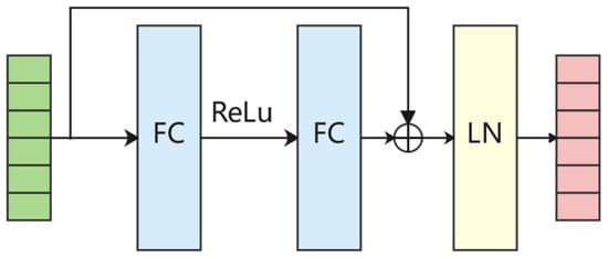
Figure 4. Multi-feature fusion module.

LN was proposed by Jimmy Lei Ba et al. in 2016. LN improves the training speed of neural networks by directly estimating normalized statistics on the total input from neurons within the hidden layer [38]. If the number of hidden points in a given fully connected layer is $H_N$ and the neuron input for the corresponding point is $\alpha$, then we can calculate the normalized statistics $\mu$ and $\sigma$ for the LN by using Equations (10) and (11):

$$\mu ={\displaystyle \frac{1}{H_N}}\sum _{i=1}^{H_N}{\alpha }_i$$

(10)

$$\sigma =\sqrt{{\displaystyle \frac{1}{H}}\sum _{i=1}^H{({\alpha }_i-\mu )}^2}$$

(11)

In order not to destroy the previous information, the LN introduces a set of gain $g$ and bias $b$ parameters, whose dimensional size is kept consistent with the output dimension, and let $f$ be the activation function. The output after the LN is shown in Equation (12):

$$h=f({\displaystyle \frac{g}{\sqrt{{\sigma }^2+\stackrel{`}{o}}}}\odot (a-\mu )+b)$$

(12)

where $\stackrel{`}{o}$ is a very small constant for the purpose of solving the division by zero problem.

3.2.4. Forecasting

The prediction layer is based on the LSTM learning fusion layer output of multiple time step vectors $\widehat{H}=({\widehat{h}}_1,{\widehat{h}}_2,\cdots ,{\widehat{h}}_l)$, and the LSTM hidden state at time $t$ is $d_t=f_d(d_{t-1},{\widehat{h}}_t)$ according to the LSTM neural network unit calculation formula given above, where $f_d$ is the LSTM calculation formula in the decoder. Its internal neurons are calculated as in Formula (4), the output vector of the last time step is used as the input of the linear fully connected layer, and a nonlinear prediction value ${\widehat{y}}_{T+\mathrm{1,1}}$ is obtained through the output of the fully connected layer.

$${\widehat{y}}_{T+\mathrm{1,1}}=V_l^T(W_l{d}_l+b_{l,1})+b_{l,1}^{\prime }$$

(13)

The final prediction of the model consists of a superposition of linear and nonlinear results.

$$\widehat{Y}={\widehat{y}}_{T+\mathrm{1,1}}+{\widehat{y}}_{T+\mathrm{1,2}}$$

(14)

4. Case Study

In this section, we first describe an empirical study in the electricity open-source dataset. We then describe the parameter settings and evaluation metrics of the model. Finally, we conduct training and testing of the model on each of the three users, along with error analysis. This paper uses a GTX3090 GPU and, four A5000 GPUs, and an Ubuntu 16.04 server environment with an I9-10100 CPU for training and testing. All code was implemented in Python 3.8, PyTorch 1.18, Sci-Learn 1.11, and other frameworks.

4.1. Datasets

The UMass Smart Dataset—2017 release [39] contains data from multiple single-family apartments, along with weather data from a nearby observation station, including temperature, humidity, atmospheric pressure, dew point, wind speed, and wind direction. In this dataset, apartment power consumption is recorded every 15 min, while weather data are recorded hourly. In this study, the power consumption data from the first 90 days of 2015 for users identified as APT14, APT16, and APT101 were selected for analysis. Temperature, humidity, and dew point were used as the meteorological features. Before training, the power consumption data were upsampled to an hourly interval using an upsampling method, and all time-series data were normalized to a 0–1 range to eliminate differences in units. Finally, each user dataset was split into training, validation, and test sets at a ratio of 8:1:1.

4.2. Performance Evaluation

In this paper, root mean square error (RMSE), mean absolute error (MAE), and mean square error (MSE) are used to assess the prediction error, with smaller values indicating more accurate model predictions.

$$MAE={\displaystyle \frac{1}{n}}\sum _{i=1}^n\left|{\widehat{y}}_i-y_i\right|$$

(15)

$$RMSE=\sqrt{{\displaystyle \frac{1}{n}}\sum _{i=1}^n{({\widehat{y}}_i-y_i)}^2}$$

(16)

$$MSE={\displaystyle \frac{1}{n}}\sum _{i=1}^n{({\widehat{y}}_i-y_i)}^2$$

(17)

where $n$ is the number of load values, $y_i$ is the true load value, and ${\widehat{y}}_i$ is the predicted value from the forecasting model.

4.3. Experimental Settings

4.3.1. Loss Function Setting

The neural network is trained by a backpropagation algorithm. In the training phase, this paper chose to use the Adam optimizer [40] to train the model through the MSE loss, with the MSE loss function formulated as follows:

$$L(\theta )={‖\widehat{y}-y‖}_2^2$$

(18)

where $\theta$ is all the trainable parameters in the model.

4.3.2. Hyperparameter Setting

The model proposed in this paper has six hyperparameter settings, subsequence length $l$, subsequence CNN output channels $O_s$, LSTM hidden dimension $E_s$, number of weather encoder output channels $O_w$, time window size $T$, and predicted LSTM network hidden state $E_d$. Set the time window length as $T=72$. For simplicity, $E_s$ and $E_d$ are set to be the same, $E_s=E_d=\left\{\mathrm{32,64,128,256}\right\}$, and a grid search is used to find the optimum. The hyperparameter settings for the remaining comparison models are shown in the table below. During training, we tested five learning rates ranging from 1 × 10⁻¹ to 1 × 10⁻⁵ with dropout set to 0 or 0.5 for each model, using early stop and setting the patience parameter to 5 to stop training when the loss in the validation set no longer decreases. Finally, we fine-tune the models for 150 epochs with a learning rate of 1 × 10⁻⁴, exponential decay of e^0.98 per step, early stop of 5, and Adam as the optimizer.

In the prediction, the final performance of the models was averaged over 10 runs for all models. In order to verify the experimental effects, five models are compared with MLP, LSTM, GRU, AE-MLP, and CNNLSTM, and a brief description of the comparison models is given in Table 1. The hyperparameter settings of the compared models are summarized in Table 2.

Table 1. Contrast model introduction.

Models	Description
MLP	Network consisting of multiple fully connected layers
LSTM	The addition of input gates, forget gates, and output gates to the RNN improves the RNN memory problem for long sequences.
GRU	A variant of the LSTM that uses reset gates and update gates to solve the gradient disappearance problem in RNNs.
AE-MLP	The encoder–decoder structure is used, with the encoder using MLP for data feature extraction and fusion, and the decoder using MLP for decoding and prediction of the encoder output codes.
CNNLSTM	Local features are extracted from the time-series data by CNN before LSTM prediction.

Table 2. Contrast model hyperparameters.

Models	Hyperparameters
MLP	Layer = 4; Hidden_size = 1024, decreasing by 1/2 layer by layer
LSTM	Layer = 2; Hidden_size = 128
GRU	Layer = 2; Hidden_size = 128
AE-MLP	Encoder: Layer = 4; Hidden_size = 1024, decreasing by 1/2 layer by layer, encoding length: 128 Decoder: Layer = 4; Hidden_size = 1024, decrementing by 1/2 layer by layer
CNNLSTM	1D-CNN: Kenerl = 3; out_channel = 16 LSTM: Layer = 2; Hidden_size = 128
Proposed Model	As the description, the model is composed of 1D-CNN, LSTM, MLP. 1D-CNN: Kenerl = 3; out_channel = 16 LSTM: Layer = 2; Hidden_size = 128 MLP: Layer = 2; Hidden_size = 128

4.4. Subsequence Partitioning and Information Compensation

The subsequence partitioning enhances the nonlinear capability of the model by changing the data dimensionality of the long series of customer electric loads, allowing the model to better learn the uncertain data features. Our work requires the prediction of residential electricity load time series in a given past $T$ time period. By dividing $T$ into $n$ equal-length subseries of length $l$ for data uncertainty special extraction, it is obvious that the value is related to the periodic characteristic of electricity use by users, and it is easy to think that 24 h is an applicable length. In order to further study the periodic characteristic, we studied the relationship between the lagging and autocorrelation coefficients of three users in 0–72 h; the peak point in the figure is the periodic relationship in the load. As shown in Figure 5, it can be seen that the autocorrelation coefficients of both APT14 and APT101 users show peak points at a lag of 24 h; in APT101, in addition to 24 h, peak points also appear at 2 h, i.e., this user takes 2 as the minimum period, while APT16 users have smaller changes in the 12–24 interval and the peak points are not significant, i.e., the periodicity is weak. Through the study of lag and autocorrelation, we have been able to select 24 as the appropriate subsequence length. To further validate the reasonableness of this subsequence division, as shown in Figure 6 and Table 3, we performed model prediction performance validation in the same conditions for subsequence lengths of 6, 9, 12, 24, and 36 in the load data of three users.

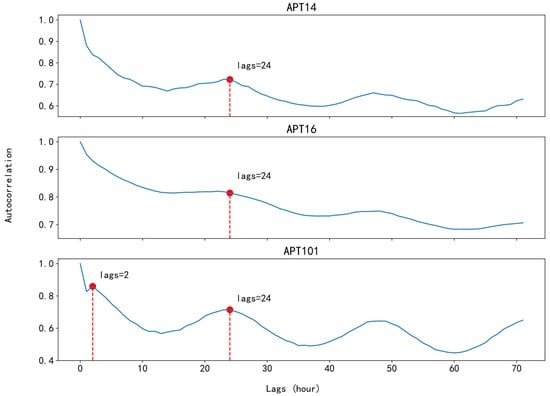
Figure 5. Hysteresis and autocorrelation coefficient.

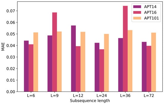
Figure 6. MAEs for different length subseries.

Table 3. Prediction performance of different subsequence length models.

	APT14			APT16			APT101
	MAE	MSE	RMSE	MAE	MSE	RMSE	MAE	MSE	RMSE
$l$ = 6	4.66 × 10−2	4.01 × 10−3	6.32 × 10−2	4.10 × 10−2	4.41 × 10−3	6.64 × 10−2	5.21 × 10−2	5.11 × 10−3	7.14 × 10−2
$l$ = 9	4.87 × 10−2	4.13 × 10−3	6.42 × 10−2	6.86 × 10−2	7.41 × 10−3	8.60 × 10−2	5.21 × 10−2	5.30 × 10−3	7.28 × 10−2
$l$ = 12	5.73 × 10−2	5.04 × 10−3	7.10 × 10−2	3.94 × 10−2	4.27 × 10−3	6.54 × 10−2	5.18 × 10−2	5.25 × 10−3	7.24 × 10−2
$l$ = 24	4.23 × 10−2	3.46 × 10−3	5.88 × 10−2	3.67 × 10−2	3.77 × 10−3	6.14 × 10−2	5.00 × 10−2	4.95 × 10−3	7.04 × 10−2
$l$ = 36	4.64 × 10−2	4.22 × 10−3	6.94 × 10−2	7.43 × 10−2	7.99 × 10−3	8.94 × 10−2	5.33 × 10−2	5.43 × 10−3	7.37 × 10−2
$l$ = 72	4.40 × 10−2	3.57 × 10−3	5.99 × 10−2	3.97 × 10−2	4.36 × 10−3	6.61 × 10−2	5.16 × 10−2	5.01 × 10−3	7.10 × 10−2

The results from multiple experiments indicate that among the three users, the model performs best when the subsequence length is set to 24, making this choice for the optimal subsequence length reasonable. Compared to the unsegmented sequence length $l$ = 72, the model with subsequence partitioning provides better predictive performance, demonstrating the model’s sensitivity to subsequence length. An inappropriate subsequence length adversely affects the model’s ability to process user power load information. Notably, for APT14, subsequence lengths of 12 and 36 yielded poor performance, which aligns with the information provided by the autocorrelation plot. For APT16, the model performs poorly at subsequence lengths of 9 and 36. Cross-referencing with the autocorrelation coefficients shows that APT16 lacks significant periodicity within a 24 h interval, with a trough at 36 h, indicating that when subsequence partitioning does not match user periodicity, the model’s inference ability decreases. A similar conclusion can be drawn for APT101, though due to the presence of a minimum cycle of 2, the model’s error range remains relatively stable across different subsequence lengths for this user.

4.5. Forecasting and Error Analysis

Based on the above parameters, the model was trained and predicted using three user data with user numbers APT14, APT16, and APT101, and the prediction results are shown in Figure 7, Figure 8 and Figure 9.

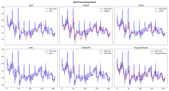
Figure 7. Prediction results of the six models for user APT14.

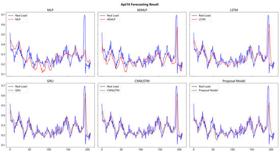
Figure 8. Prediction results for the six models of the user APT16.

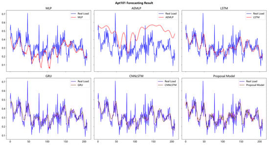
Figure 9. Prediction results for the six models of the user APT101.

Based on the error measures described above, the error analysis of the proposed model and the comparison model for the three user predictions was carried out in this paper, and the error results are shown in the following Table 4:

Table 4. Error statistics for the proposed model and the comparison model.

	APT14			APT16			APT101
	MAE	MSE	RMSE	MAE	MSE	RMSE	MAE	MSE	RMSE
MLP	5.12 × 10−2	4.59 × 10−3	6.77 × 10−2	5.20 × 10−2	5.50 × 10−3	7.42 × 10−2	7.13 × 10−2	9.47 × 10−3	9.73 × 10−2
A × 10MLP	4.68 × 10−2	4.08 × 10−3	6.38 × 10−2	5.06 × 10−2	5.54 × 10−3	7.44 × 10−2	5.52 × 10−2	5.79 × 10−3	7.61 × 10−2
GRU	4.94 × 10−2	4.45 × 10−3	6.67 × 10−2	3.83 × 10−2	4.39 × 10−3	6.63 × 10−2	5.37 × 10−2	5.30 × 10−3	7.28 × 10−2
LSTM	4.47 × 10−2	3.87 × 10−3	6.22 × 10−2	4.38 × 10−2	5.40 × 10−3	7.35 × 10−2	5.32 × 10−2	5.19 × 10−3	7.21 × 10−2
CNNLSTM	4.69 × 10−2	4.02 × 10−3	6.34 × 10−2	3.92 × 10−2	4.70 × 10−3	6.86 × 10−2	5.23 × 10−2	5.25 × 10−3	7.24 × 10−2
Our	4.23 × 10−2	3.46 × 10−3	5.88 × 10−2	3.67 × 10−2	3.77 × 10−3	6.14 × 10−2	5.00 × 10−2	4.95 × 10−3	7.04 × 10−2

The prediction errors of the model proposed in this paper for the three users of numbers APT14, APT16, and APT101 are as follows: MAE: 4.23 × 10⁻², 3.67 × 10⁻², 5.00 × 10⁻²; MSE: 3.46 × 10⁻³, 3.77 × 10⁻³, 4.95 × 10⁻³; RMSE: 5.88 × 10⁻², 6.14 × 10⁻², 7.04 × 10⁻². Compared to the five comparison models such as MLP and LSTM, our model error is optimal on all three error evaluation metrics. The forecasting results for the three users showed that direct forecasting using the fully connected MLP model was poor and the least effective of all the forecasting models; however, the results also showed that the MLP model could make predictions of upward and downward trends. The improvement in all three error indicators over direct regression using the MLP demonstrates the validity of the analysis of one indicator series by multiple fully connected networks followed by data fusion, which informs our approach to constructing external factor inputs to the data fusion. However, AEMLP is prone to overfitting, while the model has a large number of hyperparameters that make it difficult to train and debug, providing a challenge to use the model for load forecasting. Comparing the added CNN with the traditional LSTM model, the CNNLSTM model is not effective in improving the model prediction performance compared to the LSTM. Local features extracted using CNN convolution in sequences with multiple different metrics still require further processing of the local features. Our proposed model employs an input attention scheme for multiple sequences of local features extracted by the CNN, giving each feature a different weight through input attention, which works well in subsequent prediction tasks.

The error is further analyzed, and the box plot of the error distribution in Figure 10 shows that the error of our proposed model has the smallest interquartile and three-quarter interquartile range of its error distribution and the most stable error.

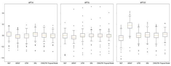
Figure 10. Prediction error distribution.

Figure 11, Figure 12 and Figure 13 present an analysis of the MAE in 24 h predictions for each of the three users. For user APT14, our proposed model shows relatively stable error levels between 13:00 and 21:00. In the case of user APT16, all models exhibit higher error rates in the first 12 h, followed by a more stable error pattern in the latter 12 h. For user APT101, the proposed model demonstrates more pronounced fluctuations in prediction error throughout the 24 h period.

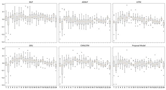
Figure 11. The 24 h error distribution of APT14 user prediction results.

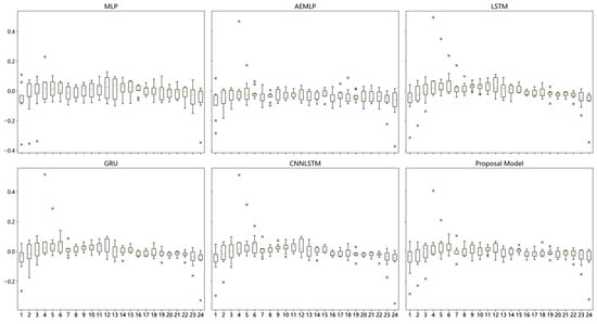
Figure 12. The 24 h error distribution of APT16 user prediction results.

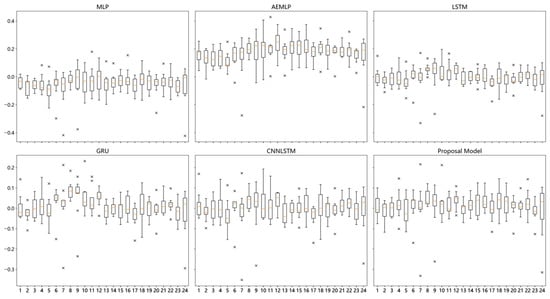
Figure 13. The 24 h error distribution of APT101 user prediction results.

By comparing the 24 h prediction error statistics of all models, the prediction stability of our proposed model is better in APT14 and APT16 users, while in APT101, the error of LSTM performs the most stable most of the time.

4.6. Ablation

As mentioned before, we introduced a meteorological feature extraction and multi-feature into the model we constructed, along with a special information compensation component and a weather factor fusion component. The data dimensionality of the input network is changed by subsequence division for feature extraction of user behavior uncertainty, but it also makes the model ignore part of the contextual information of the time-series data. Therefore, we introduce an autoregressive component for the compensation of full-text information. In the process of introducing meteorological factors into the model, we did not input them simultaneously with the electric load. Instead, we separately extracted features from the data using independent sub-networks and fused the data with the coded results from the subseries feature extraction in a structure equipped with residual connectivity and an LN mechanism. To verify the contribution of these components to the prediction performance, we performed carefully designed ablation experiments on the model with the following three sets of experiments under the conditions of the best length of the subsequence $l$ = 24 and the same hyperparameter settings above.

Case 1: Delete the information compensation component.

Case 2: No meteorological factors are introduced.

Case 3: Introduce meteorological data directly without fusion.

As is shown in Table 5, further analysis of the experimental results in Case 1 shows that adding information compensation effectively improves model prediction performance in APT14 and APT101 users, and, in APT16 users, there is no significant improvement in the MAE by adding information compensation, but there is a significant improvement in model performance by adding the information compensation component in the MSE and RMSE errors. The results in Case 1 demonstrate that although the results in Case 1 show the improvement in model capability by information compensation is small in some cases, the information compensation component is still effective in improving the model results in several error metrics. Overall, the introduction of the information compensation component enhances the stability of the model and effectively improves the overall performance of the model.

Table 5. Errors in ablation experiments.

	APT14			APT16			APT101
	MAE	MSE	RMSE	MAE	MSE	RMSE	MAE	MSE	RMSE
Case 1	4.70 × 10−2	3.71 × 10−3	6.09 × 10−2	3.68 × 10−2	4.14 × 10−3	6.44 × 10−2	5.38 × 10−2	5.25 × 10−3	7.25 × 10−2
Case 2	4.61 × 10−2	3.99 × 10−3	6.32 × 10−2	4.58 × 10−2	5.00 × 10−3	7.07 × 10−2	5.33 × 10−2	5.71 × 10−3	7.68 × 10−2
Case 3	4.36 × 10−2	3.52 × 10−3	5.94 × 10−2	4.11 × 10−2	4.21 × 10−3	6.48 × 10−2	5.25 × 10−2	5.40 × 10−3	7.35 × 10−2

Comparing the results of Case 2 and Case 3shows that the introduction of meteorological data can improve the prediction ability of our proposed model. The analysis of the results of Case 3 shows that the prediction model without the multifactor fusion layer has an increase in the values of the MAE, MSE, and RMSE when compared with the prediction model with the multifactor fusion layer proposed in this paper; in APT14 users, the removal of the multifactor fusion process has less impact on the prediction results, while, in APT16 and APT14 users, removing the fusion layer has less impact on the prediction results. However, in APT16 and APT101, removing the fusion layer has a greater impact on the prediction performance, which proves that for meteorological sensitive users, the introduced multifactor fusion layer can improve the model performance, while, for users who are not sensitive to meteorological data, adding meteorological data can also improve the fault tolerance of the model and ensure the prediction performance.

4.7. Complexity and Scalability

During training, the LSTM model took 102 min, the CNN-LSTM model took 114 min, and the proposed model took 217 min. Due to the more complex model structure, the proposed model’s training time is approximately twice that of the LSTM and CNN-LSTM models. Moreover, the model’s design incorporates a 1D CNN module for extracting external features and a residual-based fusion module for integration, showcasing its scalability in adapting to additional features effectively.

5. Conclusions

This paper presents a short-term residential electricity load forecasting model based on the fusion of customer load uncertainty feature extraction and meteorological factors. The model first performs subsequence partitioning and alignment for long sequences of customer electricity loads, processes local features using the CNN, and captures the customer’s electricity consumption behavior over historical periods using an input attention mechanism. Meanwhile, for external meteorological factors, the input data were preprocessed with first-order differences, and a CNN model was subsequently used for feature extraction and coding. In the feature fusion layer, user load features and meteorological factors are fused on a time-step-by-time basis in a fusion module based on residual connections, and, finally, the fused data are predicted using an LSTM network with an autoregressive module. The best performance of the proposed model was verified by testing the user load on the real UMASS dataset and comparing it with five benchmark models, MLP, LSTM, GRU, AEMLP, and CNNLSTM.

However, only meteorological factors are used in this paper for external influences on customer behavior; social and calendar factors should also be taken into account for customer load forecasting, and the length of the subseries used in this paper is a fixed 24 h. Therefore, in future work, we will try to integrate the calendar factors and the social information factors as a method to solve the model overfitting and improve the prediction accuracy. We will also explore the impact of variable-length subseries and other user load uncertainty analysis methods on the model accuracy.

References

- Wang, S.; Chen, H.; Wu, L.; Wang, J. A novel smart meter data compression method via stacked convolutional sparse auto-encoder. Int. J. Electr. Power Energy Syst. 2020, 118, 105761. [Google Scholar] [CrossRef]
- Raza, A.; Jingzhao, L.; Ghadi, Y.; Adnan, M.; Ali, M. Smart home energy management systems: Research challenges and survey. Alex. Eng. J. 2024, 92, 117–170. [Google Scholar] [CrossRef]
- O’Donnell, J.; Su, W. Attention-Focused Machine Learning Method to Provide the Stochastic Load Forecasts Needed by Electric Utilities for the Evolving Electrical Distribution System. Energies 2023, 16, 5661. [Google Scholar] [CrossRef]
- Wu, F.; Cattani, C.; Song, W.; Zio, E. Fractional ARIMA with an improved cuckoo search optimization for the efficient Short-term power load forecasting. Alex. Eng. J. 2020, 59, 3111–3118. [Google Scholar] [CrossRef]
- Aflaki, A.; Gitizadeh, M.; Kantarci, B. Accuracy improvement of electrical load forecasting against new cyber-attack architectures. Sustain. Cities Soc. 2022, 77, 103523. [Google Scholar] [CrossRef]
- Heng, S.; Minghao, X.; Ran, L. Deep Learning for Household Load Forecasting—A Novel Pooling Deep RNN. IEEE Trans. Smart Grid 2018, 9, 5271–5280. [Google Scholar] [CrossRef]
- Danish, M.S.S.; Ahmadi, M.; Ibrahimi, A.M.; Dinçer, H.; Shirmohammadi, Z.; Khosravy, M.; Senjyu, T. Data-Driven Pathways to Sustainable Energy Solutions; Springer Nature: Cham, Switzerland, 2024; Volume 2024, pp. 1–31. [Google Scholar] [CrossRef]
- Wang, Y.; Chen, Q.; Hong, T.; Kang, C. Review of Smart Meter Data Analytics: Applications, Methodologies, and Challenges. IEEE Trans. Smart Grid 2019, 10, 3125–3148.6. [Google Scholar] [CrossRef]
- Aseeri, A.O. Effective RNN-Based Forecasting Methodology Design for Improving Short-Term Power Load Forecasts: Application to Large-Scale Power-Grid Time Series. J. Comput. Sci. 2023, 68, 101984. [Google Scholar] [CrossRef]
- Yu, P.; Fang, J.; Xu, Y.B.; Shi, Q. Application of Variational Mode Decomposition and Deep Learning in Short-Term Power Load Forecasting. J. Phys. Conf. Ser. 2021, 1883, 012128. [Google Scholar] [CrossRef]
- Wang, J.; Du, Y.; Wang, J. LSTM based long-term energy consumption prediction with periodicity. Energy 2020, 197, 117197. [Google Scholar] [CrossRef]
- Kong, W.; Dong, Z.; Jia, Y.; Hill, D.; Xu, Y.; Zhang, Y. Short-Term Residential Load Forecasting Based on LSTM Recurrent Neural Network. IEEE Trans. Smart Grid 2019, 10, 841–851. [Google Scholar] [CrossRef]
- Cho, K.; van Merrienboer, B.; Gülçehre, Ç.; Bougares, F.; Schwenk, H.; Bengio, Y. Learning Phrase Representations using RNN Encoder-Decoder for Statistical Machine Translation. arXiv 2014, arXiv:1406.1078. [Google Scholar] [CrossRef]
- Wang, Y.; Liu, M.; Bao, Z.; Zhang, S. Short-Term Load Forecasting with Multi-Source Data Using Gated Recurrent Unit Neural Networks. Energies 2018, 11, 1138. [Google Scholar] [CrossRef]
- Hossen, T.; Nair, A.; Chinnathambi, R.; Ranganathan, P. Residential Load Forecasting Using Deep Neural Networks (DNN). In Proceedings of the 2018 North American Power Symposium (NAPS), Fargo, ND, USA, 9–11 September 2018; pp. 1–5. [Google Scholar] [CrossRef]
- Tang, X.; Dai, Y.; Liu, Q.; Dang, X.; Xu, J. Short-term Power Load Prediction Based on Multilayer Bidirectional Recurrent Neural Network. Power Capacit. React. Power Compens. 2022, 43, 96–104. [Google Scholar] [CrossRef]
- Pavlatos, C.; Makris, E.; Fotis, G.; Vita, V.; Mladenov, V. Enhancing Electrical Load Prediction Using a Bidirectional LSTM Neural Network. Electronics 2023, 12, 4652. [Google Scholar] [CrossRef]
- Zou, Z.; Wang, J.; E, N.; Zhang, C.; Wang, Z.; Jiang, E. Short-Term Power Load Forecasting: An Integrated Approach Utilizing Variational Mode Decomposition and TCN–BiGRU. Energies 2023, 16, 6625. [Google Scholar] [CrossRef]
- Zhang, M.; Zhou, Y.; Xu, Z. Short-Term Load Forecasting Using Recurrent Neural Networks with Input Attention Mechanism and Hidden Connection Mechanism. IEEE Access 2020, 8, 186514–186529. [Google Scholar] [CrossRef]
- Rahman, A.; Srikumar, V.; Smith, A. Predicting electricity consumption for commercial and residential buildings using deep recurrent neural networks. Appl. Energy 2018, 212, 372–385. [Google Scholar] [CrossRef]
- Liu, T.; Tan, Z.; Xu, C.; Chen, H.; Li, Z. Study on deep reinforcement learning techniques for building energy consumption forecasting. Energy Build. 2020, 208, 109675. [Google Scholar] [CrossRef]
- Kim, T.; Cho, S. Predicting residential energy consumption using CNN-LSTM neural networks. Energy 2019, 182, 72–81. [Google Scholar] [CrossRef]
- Zang, H.; Xu, R.; Cheng, L.; Ding, T.; Liu, L.; Wei, Z.; Sun, G. Residential load forecasting based on LSTM fusing self-attention mechanism with pooling. Energy 2021, 229, 120682. [Google Scholar] [CrossRef]
- Chen, H.; Wang, S.; Wang, S.; Li, Y. Day-ahead aggregated load forecasting based on two-terminal sparse coding and deep neural network fusion. Electr. Power Syst. Res. 2019, 177, 105987. [Google Scholar] [CrossRef]
- Khan, Z.; Hussain, T.; Ullah, A.; Rho, S.; Lee, M.; Baik, S. Towards Efficient Electricity Forecasting in Residential and Commercial Buildings: A Novel Hybrid CNN with a LSTM-AE based Framework. Sensors 2020, 20, 1399. [Google Scholar] [CrossRef]
- Hosein, S.; Hosein, P. Load forecasting using deep neural networks. In Proceedings of the 2017 IEEE Power & Energy Society Innovative Smart Grid Technologies Conference (ISGT), Torino, Italy, 26–29 September 2017; pp. 1–5. [Google Scholar] [CrossRef]
- Geng, G.; He, Y.; Zhang, J.; Qin, T.X.; Yang, B. Short-Term Power Load Forecasting Based on PSO-Optimized VMD-TCN-Attention Mechanism. Energies 2023, 16, 4616. [Google Scholar] [CrossRef]
- Cui, J.; Li, Y.; Liu, J.L.; Li, J.; Yang, Z.; Yin, C.L. Efficient Self-attention with Relative Position Encoding for Electric Power Load Forecasting. J. Phys. Conf. Ser. 2022, 2205, 012009. [Google Scholar] [CrossRef]
- Gou, Y.; Guo, C.; Qin, R. Ultra short term power load forecasting based on the fusion of Seq2Seq BiLSTM and multi head attention mechanism. PLoS ONE 2024, 19, e0299632. [Google Scholar] [CrossRef]
- Wu, Y.; Zhang, Z. Attention-BiLSTM Short-Term Electricity Load Forecasting Based on Sparrow Search Optimization. Process Autom. Instrum. 2023, 44, 91–95. [Google Scholar] [CrossRef]
- Qin, Y.; Song, D.; Chen, H.; Cheng, W.; Jiang, G.; Cottrell, G. A Dual-Stage Attention-Based Recurrent Neural Network for Time Series Prediction. arXiv 2017, arXiv:1704.02971. [Google Scholar] [CrossRef]
- Maryam, I. Electrical load-temperature CNN for residential load forecasting. Energy 2021, 227, 120480. [Google Scholar] [CrossRef]
- Wang, Y.; Zhang, N.; Chen, X. A Short-Term Residential Load Forecasting Model Based on LSTM Recurrent Neural Network Considering Weather Features. Energies 2021, 14, 2737. [Google Scholar] [CrossRef]
- Lecun, Y.; Bottou, L.; Bengio, Y.; Haffner, P. Gradient-based learning applied to document recognition. Proc. IEEE 1998, 86, 2278–2324. [Google Scholar] [CrossRef]
- Abdeljaber, O.; Avci, O.; Kiranyaz, S.; Gabbouj, M.; Inman, D. Real-time vibration-based structural damage detection using one-dimensional convolutional neural networks. J. Sound Vib. 2017, 388, 154–170. [Google Scholar] [CrossRef]
- Chen, K.; Chen, F.; Lai, B.; Jin, Z.; Liu, Y.; Li, K. Dynamic Spatio-Temporal Graph-Based CNNs for Traffic Flow Prediction. IEEE Access 2020, 8, 185136–185145. [Google Scholar] [CrossRef]
- He, K.; Zhang, X.; Ren, S.; Sun, J. Deep residual learning for image recognition. In Proceedings of the 2016 IEEE Conference on Computer Vision and Pattern Recognition (CVPR), Las Vegas, NV, USA, 27–30 June 2016; pp. 770–778. [Google Scholar] [CrossRef]
- Ba, L.; Kiros, R.; Hinton, G. Layer Normalization. arXiv 2016, arXiv:1607.06450. [Google Scholar] [CrossRef]
- Smart—UMass Trace Repository. Available online: https://traces.cs.umass.edu/docs/traces/smartstar (accessed on 21 April 2022).
- Kingma, D.; Ba, J. Adam: A method for stochastic optimization. arXiv 2017, arXiv:1412.6980. [Google Scholar] [CrossRef]
Disclaimer/Publisher’s Note: The statements, opinions and data contained in all publications are solely those of the individual author(s) and contributor(s) and not of MDPI and/or the editor(s). MDPI and/or the editor(s) disclaim responsibility for any injury to people or property resulting from any ideas, methods, instructions or products referred to in the content. |
© 2025 by the authors. Licensee MDPI, Basel, Switzerland. This article is an open access article distributed under the terms and conditions of the Creative Commons Attribution (CC BY) license (https://creativecommons.org/licenses/by/4.0/).