Evaluating Municipal Solid Waste Incineration Through Determining Flame Combustion to Improve Combustion Processes for Environmental Sanitation

Abstract

Municipal solid waste (MSW) refers to solid and semi-solid waste generated during human production and daily activities. The process of incinerating such waste, known as municipal solid waste incineration (MSWI), serves as a critical method for reducing waste volume and recovering resources. Automatic online recognition of flame combustion status during MSWI is a key technical approach to ensuring system stability, addressing issues such as high pollution emissions, severe equipment wear, and low operational efficiency. However, when manually selecting optimized features and hyperparameters based on empirical experience, the MSWI flame combustion state recognition model suffers from high time consumption, strong dependency on expertise, and difficulty in adaptively obtaining optimal solutions. To address these challenges, this article proposes a method for constructing a flame combustion state recognition model optimized based on reinforcement learning (RL), long short-term memory (LSTM), and parallel differential evolution (PDE) algorithms, achieving collaborative optimization of deep features and model hyperparameters. First, the feature selection and hyperparameter optimization problem of the ViT-IDFC combustion state recognition model is transformed into an encoding design and optimization problem for the PDE algorithm. Then, the mutation and selection factors of the PDE algorithm are used as modeling inputs for LSTM, which predicts the optimal hyperparameters based on PDE outputs. Next, during the PDE-based optimization of the ViT-IDFC model, a policy gradient reinforcement learning method is applied to determine the parameters of the LSTM model. Finally, the optimized combustion state recognition model is obtained by identifying the feature selection parameters and hyperparameters of the ViT-IDFC model. Test results based on an industrial image dataset demonstrate that the proposed optimization algorithm improves the recognition performance of both left and right grate recognition models, with the left grate achieving a 0.51% increase in recognition accuracy and the right grate a 0.74% increase.

1. Introduction

Pollution control and prevention are crucial for the sustainable development of the global economy, the protection of the environment, and the safeguarding of public health, making them a global priority [1,2]. Municipal solid waste (MSW) is growing annually by 8% to 10% worldwide [3,4]. In developing countries such as China, many cities are at risk of being overwhelmed by MSW, leading to significant environmental challenges [5]. MSW incineration (MSWI) is a complex system that converts waste into energy (WTE) and plays a key role in addressing urban environmental issues [6,7,8] while supporting renewable energy recycling [9]. Although MSWI is a scientifically validated waste treatment method, emissions from these plants are a major source of pollution [10,11], often facing opposition due to the “Not in My Backyard” (NIMBY) effect [12,13]. The combustion stage of the MSWI process is the primary source of environmental indicators (EIs) such as NOx, CO, HCl, and SO₂ [14]. Flame combustion state recognition technology enables early detection of abnormal combustion conditions, thereby guiding the control system to promptly adjust operational parameters such as grate speed and facilitating a rapid return to normal combustion. Under abnormal conditions, incomplete fuel combustion leads to increased carbon monoxide emissions, a significantly higher risk of dioxin formation due to suboptimal combustion environments, and reduced power generation efficiency [3]. Furthermore, deteriorating conditions may even cause unplanned shutdowns and equipment wear. Therefore, accurate identification of flame combustion states is crucial for pollution reduction and optimized control.

Due to differences in operating equipment, the uncertainty in the maintenance of MSWI plants, fluctuations in the composition of MSW, and strong interference from the environment within the incinerator, accurately identifying the flame combustion state is challenging [3]. Additionally, the reliance on experts for manual recognition of combustion status lacks stability, making it difficult to ensure consistent operational efficiency and pollution reduction in the MSWI process [15]. The process of expert manual identification is intelligently modeled by constructing a data-driven mapping function from image space to state space, thereby transforming human visual experience based on prior knowledge into a computable and optimizable mathematical model. Leveraging the powerful representational learning capability of deep neural networks, discriminative deep-level information is automatically extracted from raw data, and high-precision modeling is achieved by learning the underlying complex patterns and decision boundaries. By building a high-accuracy artificial intelligence-based combustion state recognition model, limitations of human experts—such as subjectivity, limited experience, and cognitive biases—are overcome in terms of generalization, robustness, and judgment consistency. This provides effective support for the intelligent operation of the MSWI process.

Extensive research has been conducted on the identification of MSWI flame combustion states. Zhou et al. proposed a PCA-K-means clustering approach to distinguish between abnormal and normal flames, using only two states for classification [16]. Huang, on the other hand, extracted key parameters—such as the grayscale mean, flame area ratio, and flame high-temperature rate—from combustion images through image processing technology. These parameters were then input into K-nearest neighbor (KNN) and convolutional neural network (CNN) models for partial burning state recognition [17]. However, this approach relies on only a few physical features. Zhou also extracted 12 physical features from flame images based on expert knowledge and used a backpropagation neural network (BPNN) for combustion state recognition [18]. Additionally, Qiao et al. constructed a combustion state recognition model based on flame image color moment features and applied the least squares support vector machine (LS-SVM) [19]. Guo et al. took a different approach by generating abnormal working condition images using deep convolutional adversarial networks (DCGANs) to construct a CNN for combustion state recognition. This method addresses the issue of limited abnormal combustion images [20]. However, it only classifies combustion states based on the position of the combustion line, which provides limited local information. In contrast, Pan et al. created a flame combustion state recognition database using global image features and employed an improved visual transformer-based deep forest classification (ViT-IDFC) algorithm for state recognition [21]. The key limitation of the research on MSWI flame state recognition models mentioned above is that determining hyperparameters often requires expert experience and repeated experimentation, which is time-consuming, resource-intensive, and computationally expensive. Furthermore, these methods do not guarantee that the model will achieve optimal recognition performance.

To address these issues, this article conducts research on flame combustion state recognition through the collaborative optimization of deep features and model hyperparameters. Evolutionary algorithms (EAs) are commonly used to solve the aforementioned optimization problems [22]. Among all possible combinations, EAs can achieve the search for a globally optimal or near-optimal solution, thereby enabling the model to reach its best performance. The optimization process simulates the mechanisms of “natural selection” and “genetic inheritance” observed in biological systems. Each “population” consists of multiple potential solutions, and the algorithm iteratively performs operations such as selection, crossover, and mutation. Based on the evaluation results of each solution, superior individuals are retained while inferior ones are eliminated, gradually evolving solutions with progressively improved performance. Among these, the Differential Evolution (DE) algorithm is a heuristic optimization technique primarily used to solve continuous problems in real space. Due to its automatic adaptation and ease of implementation, DE has been widely adopted. For example, Dilbag et al. optimized the hyperparameters of a remote sensing image visibility restoration model using dynamic DE [23], Singh et al. adjusted the initial parameters of a CNN using multi-objective DE [24], and Chen et al. introduced Gaussian–Cauchy mutation and parameter adaptation strategies in DE to solve the economic scheduling problem of large-scale cogeneration systems [25]. These studies achieved improved results by optimizing model parameters using the DE algorithm. However, DE faces challenges such as stagnation and premature convergence during the optimization process, which are closely linked to the control parameters and the crossover rate of the algorithm. Clearly, for different optimization problems, the most suitable parameter settings must strike a balance between maintaining population diversity and enhancing convergence speed. Typically, the control parameters of DE are set based on optimization experience obtained through repeated experiments.

Reinforcement learning (RL) achieves task goals through interactive learning between agents and the environment [26]. Unlike supervised and unsupervised learning, RL focuses on decision-making based on environmental feedback. In the RL framework, agents learn to maximize long-term cumulative rewards through interaction with the environment. Its advantages include the ability to make sequential decisions, adapt to environmental changes, balance exploration and exploitation, not requiring large amounts of labeled data, and having high generalizability [27]. Currently, RL is gradually becoming an important tool for solving model hyperparameter optimization. For example, Pan et al. designed a deep neural network, PFSPNet [28], to achieve an end-to-end output model that is not limited by problem size, aimed at solving the schedule ng problem in an assembly line workshop. They applied a deep RL execution evaluation strategy to optimize the network parameters of the model. The results showed that this approach outperformed existing heuristic algorithms. Tian et al. addressed the exploration and exploitation challenges faced by EAs in operator selection during the search process [29]. They treated decision variables as states and candidate operators as actions, using deep neural networks to learn and estimate the Q-value strategy for each action in a given state. Based on reinforcement learning, their proposed method was used for operator selection. Experimental results demonstrated that the method could successfully identify the optimal operator for each parent.

Furthermore, some scholars are focused on exploring how to combine RL with DE in the search process to achieve adaptive selection of optimal parameters. For example, Hu et al. proposed integrating RL with DE in photovoltaic models [30], evaluating fitness function values during iterations to determine action rewards for adjusting parameter values, and then using RL to adjust these parameters to identify the most suitable algorithm settings for the environmental model. Tan et al. introduced a hybrid mutation strategy DE algorithm based on deep Q-network (DQN) [31], called DEDQN, which implements adaptive selection of mutation strategies during the evolutionary process through RL. Sun et al. used Long Short-Term Memory (LSTM) as the parameter controller for DE and employed an RL algorithm to optimize the parameters of the LSTM [32]. These studies leverage the reward/punishment mechanism of RL, enabling agents to continuously learn the optimal parameter combinations through trial and error, thereby improving model performance. However, there is a lack of research on improving the operational efficiency of the DE algorithm and on performing deep feature and model hyperparameter collaborative optimization in the context of flame combustion state recognition.

In the MSWI process, variations in process parameters such as MSW heating value and air supply volume directly influence the flame combustion state, which manifests as differences in flame image data distribution. Building on prior knowledge from field experts, reference [21] proposed a global feature-oriented flame combustion state image dataset and introduced the ViT-IDFC recognition algorithm. However, the multilayer feature selection and hyperparameter determination of this model mainly depend on manual experience. When the distribution of the flame combustion state dataset changes, the effectiveness of manual parameter selection decreases significantly. Thus, there is a need to develop a method capable of adaptively selecting hyperparameters based on changes in dataset distribution. This approach ensures that when process parameter variations such as MSW heating value or air supply volume cause a decline in model recognition accuracy, this performance degradation signal promptly triggers the optimization framework, driving it to automatically adjust feature selection parameters and model hyperparameters to regain adaptation to new operating conditions. To improve the performance of the flame global characterization information combustion state recognition model for MSWI processes, it is crucial to address the following: (1) how to select appropriate feature selection parameters and recognition model hyperparameters for encoding, and (2) how to optimize the control parameters of the parallel DE (PDE) algorithm to accommodate changes in the image dataset distribution. parameters of the parallel differential evolution algorithm to adapt to changes in image dataset distribution.

In response to the above challenges, this article proposes a ViT-IDFC recognition model optimized by RL-LSTM-PDE. First, the hyperparameter selection process of the ViT-IDFC combustion state recognition model is encoded as a PDE optimization problem. Next, control parameters—such as the mutation factor and crossover factor of PDE—are modeled using LSTM, with the LSTM output providing the optimal hyperparameters for the ViT-IDFC combustion state recognition model. Finally, the network parameters of the LSTM model are derived through PDE during the empirical learning process, which optimizes both ViT features and IDFC model hyperparameters. The innovations of this article are as follows: (1) a novel optimization modeling strategy for deep features and model hyperparameters, which formalizes the selection process as an observable Markov Decision Process (MDP); (2) the use of a multi-layer optimization approach, combining PDE for model parameter optimization, LSTM for predicting the evolutionary parameters of PDE, and RL for optimizing PDE parameters based on model generalization performance, to solve the MDP problem; (3) the collaborative optimization of ViT-IDFC model features and hyperparameters in the MSWI process, which improves the model’s generalization performance.

2. Flame State Recognition Description for MSWI Process

The process flow of grate furnace type MSWI is shown in Figure 1.

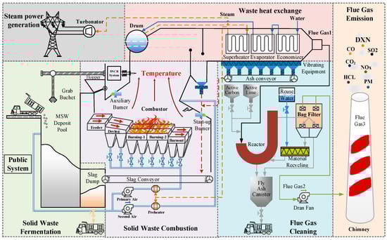
Figure 1. MSWI process flow.

As shown in Figure 1, the MSWI process is a complex, serial system consisting of six stages: solid waste fermentation, solid waste combustion, waste heat exchange, steam power generation, flue gas treatment, and flue gas emissions. These stages are interrelated and together form the overall framework of the MSWI process. Among them, solid waste combustion is the core of the entire MSWI process, and the assessment of the on-site MSW combustion status is generally based on domain experts’ visual observation of flame images. Correspondingly, the combustion control strategy is adjusted based on the combustion status.

The schematic diagram of the four combustion states of MSW based on global information is shown in Figure 2.

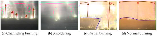
Figure 2. Typical flame combustion states during MSWI process.

In Figure 2, the blue line represents the burnout line of the flame, the red line represents the edge of the flame, and the red arrow indicates the direction and height of the flame. As shown in Figure 2, the combustion state of the MSWI is primarily classified into four categories: channeling burning, smoldering, partial burning, and normal burning. Significant differences are observed in the distribution of burnout lines, flame edges, direction, and height across the different combustion states, which result from the combined effects of the current combustion control strategies and the components of the MSW.

3. Optimization Modeling Strategy

The optimization modeling strategy proposed in this article is shown in Figure 3.

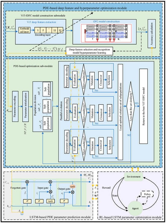
Figure 3. Optimization modeling strategy.

In Figure 3, ${\left\{{\mathit{X}}_n\right\}}_{n=1}^N$ and ${\left\{y_n\right\}}_{n=1}^N$ represent the flame image dataset and its corresponding combustion state, respectively; $[S_P^1,S_P^2,\cdots ,S_P^{12}]$ represents the deep feature selection parameters of the ViT-IDFC combustion state recognition model submodule; $M$ and $J$ represent model hyperparameters such as the number of decision trees and the minimum number of partition samples for leaf nodes in IDFC; ${\mathsf{\Theta }}_F^t$ and ${\mathsf{\Theta }}_{\mathrm{CR}}^t$ represent the mutation factor and crossover factor of PDE; and $\mathit{W}$ represents the network parameter of LSTM.

The functions of each module are as follows:

(1)

PDE-based deep feature and hyperparameter optimization module: encodes the feature selection parameters $[S_P^1,S_P^2,\cdots ,S_P^{12}]$ and recognition model hyperparameters $M$ and $J$ of ViT-IDFC as decision variables for PDE optimization, and the fitness is characterized by the recognition;

(2)

LSTM-based PDE parameter prediction module: an LSTM model is constructed, with the mutation factor $F$ and crossover factor $Cr$ of PDE as inputs, and optimized $F^{*}$ and $C{r}^{*}$ as the outputs;

(3)

RL-based LSTM parameter optimization module: treating LSTM as a Markov decision process and using RL optimization based on policy gradient algorithm to obtain the optimized control parameters of PDE.

Therefore, the optimization modeling process is as follows. Firstly, based on RL agents that can learn from experience, we obtain the network parameters of LSTM. Then, based on LSTM, we determine the $F$ and $Cr$ parameters of PDE. Next, based on PDE, we determine the parameters of the ViT-IDFC model, such as $[S_P^1,S_P^2,\cdots ,S_P^{12}]$, $M$ and $J$. Finally, we obtain the optimized recognition model.

4. Algorithm Implementation

4.1. PDE-Based Deep Feature and Hyperparameter Optimization Module

4.1.1. ViT-IDFC Model Construction Submodule

Firstly, a combustion state recognition model based on ViT-IDFC is constructed, and the collected flame images on site are classified to obtain a flame image dataset, which is denoted as ${({\mathit{X}}_n,y_n)}_{n=1}^N$ (where ${\mathit{X}}_n\in R^{H\times W\times C}$ represents the $n\mathrm{th}$ image, $H$, $W$ and $C$ respectively represent its height, width, and number of channels, $y_n$ represents the label, and $N$ represents the sample size of the dataset). On this basis, pre-training of ViT is carried out based on the ImageNet dataset, and the ViT model is iteratively optimized until the network performance meets the predetermined requirements. The weights and bias parameters of the model are saved. Based on the above image dataset, transfer feature extraction is performed by inputting the flame image dataset ${({\mathit{X}}_n^{\mathrm{Flame}})}_{n=1}^N$ into the ViT model. Further, the feature sequences extracted by each encoding layer based on Transformer is represented using the following equation:

$${[P_n^1, P_n^2, \cdots , P_n^{12}]}_{n=1}^N=f_{\mathrm{ViT}}{({\mathit{X}}_n^{\mathrm{Flame}})}_{n=1}^N$$

(1)

where $f_{\mathrm{ViT}}(·)$ represents the ViT deep feature extraction model composed of an embedding layer and an encoding layer.

Next, transfer feature selection is performed based on expert experience, and the selected flame image depth features are denoted as ${(P_n^{*-12})}_{n=1}^N$. Furthermore, we construct the IDFC module and concatenate ${({\mathit{X}}_n^{\mathrm{Flame},\mathrm{samll}})}_{n=1}^N$ obtained by reducing ${(P_n^{*-12})}_{n=1}^N$ and ${({\mathit{X}}_n^{\mathrm{Flame}})}_{n=1}^N$ to obtain the following features:

$${(z_n^{\mathrm{Flame}})}_{n=1}^N={[P_n^{*-12},\mathrm{flatten}(X_n^{\mathrm{Flame},\mathrm{small}})]}_{n=1}^N$$

(2)

where $\mathrm{flatten}(·)$ represents the image flattening operation.

Finally, the recognition result is obtained by inputting ${(z_n^{\mathrm{Flame}})}_{n=1}^N$ into the IDFC model as follows:

$${({\widehat{y}}_n^{\mathrm{Flame}})}_{n=1}^N=f_{\mathrm{IDFC}}({(z_n^{\mathrm{Flame}})}_{n=1}^N)$$

(3)

where $f_{\mathrm{IDFC}}(·)$ represents the constructed IDFC model.

4.1.2. PDE-Based Optimization Sub-Module

DE is widely used to solve global optimal solutions in multidimensional spaces. To improve the problem of long optimization time in DE, the PDE algorithm uses multiple population parallelization and reduces the size of subpopulations to reduce evolution time, while further improving evolution efficiency by constraining the direction of subpopulation evolution in iterations [33]. It can be divided into four parts, i.e., optimization parameter encoding, parameter initialization, population partition, and parallel evolution. Details are shown as follows.

Step (1) Optimization parameter encoding. The deep feature ${[P_n^1, P_n^2, \cdots , P_n^{12}]}_{n=1}^N$ in the ViT-IDFC recognition model represents the 12 layers of features extracted by the ViT model. Obviously, relying on expert experience to select features has a certain degree of subjective arbitrariness. To further select deep features that can represent global information, $[S_P^1,S_P^2,\cdots ,S_P^{12}]$ is used as the parameter for selecting deep features. We take the first layer feature as example; the criterion is defined as follows: when $S_P^1=1$ is present, it is selected; when $S_P^1=0$ occurs, it is deleted. In addition, the number of decision trees $J$ and the minimum number of leaf nodes $M$ of the base learner RF in the IDFC recognition model are encoded as model hyperparameters.

Step (2) Parameter initialization. Four PDE parameters, including population size $f_{\mathrm{size}}(NP)$, number of subpopulations $A$, subpopulation mutation factor $F$, and subpopulation crossover probability $CR$, need to be initialized, where $f_{\mathrm{size}}(NP)$ and $A$ are used to partition subpopulations; $F$ and $CR$ are used for the evolutionary process of each subpopulation. We use prediction accuracy as the fitness function to evaluate the fitness of the population, which is as follows:

$${\mathrm{Fitness}}_{NP}=f_{\mathrm{Accuracy}}(NP)$$

(4)

where $f_{\mathrm{Accuracy}}(·)$ represents the fitness evaluation function.

Step (3) population partition. Randomly dividing the initial population into $A$ subpopulations can be expressed as:

$$\{sub\_N{P}_1,\cdots ,sub\_N{P}_{\alpha },\cdots ,sub\_N{P}_{\mathrm{A}}\}=f_{\mathrm{random}}(NP,A)$$

(5)

The size of the $\alpha \mathrm{th}$ subpopulation $sub\_N{P}_{\alpha }$ is obtained as follows:

$$f_{\mathrm{size}}(sub\_N{P}_{\alpha })={\displaystyle \frac{1}{A}}{f}_{\mathrm{size}}(NP)$$

(6)

Step (4) Parallel evolution. We execute DE in parallel pools for different subpopulations based on their partitioning results. The following sections describe the process from two aspects such as independent evolution of subpopulations and overall evolution of the population.

a.

Independent evolution of subpopulations

The evolutionary strategy of subpopulations is consistent with the standard DE strategy and can be divided into three parts such as “mutation”, “crossover”, and “selection”. The following section takes the $t\mathrm{th}$ generation of the $\alpha \mathrm{th}$ subpopulation as an example.

Firstly, we adopt the DE/current to best/1 strategy for mutation operation. Specifically, two different individuals are differentiated and added to a third individual to obtain a mutated individual, as shown below:

$$\begin{array}{c}{\mathrm{V}}_{\alpha }^m(t+1)=sub\_N{P}_{\alpha }^m(t)+{\mathsf{\Theta }}_F^t(sub\_N{P}_{\alpha }^{\mathrm{best}}(t)-sub\_N{P}_{\alpha }^m(t))+\\ {\mathsf{\Theta }}_F^t(sub\_N{P}_{\alpha }^{r1}(t)-sub\_N{P}_{\alpha }^{r2}(t))\end{array}$$

(7)

where ${\mathsf{\Theta }}_F^t$ represents the variable factor, ${\mathsf{\Theta }}_F^t=\{F^t,0<F^t\le 1\}$; ${\mathrm{V}}_{\alpha }^m(t+1)$ represents the $m\mathrm{th}$ mutant individual of the $(t+1)\mathrm{th}$ generation; $sub\_N{P}_{\alpha }^m(t)$ represents the $m\mathrm{th}$ individual of the $t\mathrm{th}$ generation; $sub\_N{P}_{\alpha }^{r1}(t)$ and $sub\_N{P}_{\alpha }^{r2}(t)$ represent two random individuals of the $t\mathrm{th}$ generation; and $sub\_N{P}_{\alpha }^{\mathrm{best}}(t)$ is the optimal individual of the $t\mathrm{th}$ generation.

Here, the mutation operation of the PDE algorithm is referred to as a function $\mathbf{M}(·)$, and the generation process of the $t\mathrm{th}$ generation mutation heterogeneous group ${\mathrm{V}}_{\alpha }(t+1)$ is as follows:

$${\mathrm{V}}_{\alpha }(t+1)=\mathbf{M}(sub\_N{P}_{\alpha }(t);{\mathsf{\Theta }}_F^t)$$

(8)

Next, we perform crossover operations on each individual and their offspring’s mutated individuals. Here, the $m\mathrm{th}$ individual of the $(t+1)\mathrm{th}$ is represented as:

$$U_{\alpha }^m(t+1)=\{S_{P,m}^1,S_{P,m}^2,\cdots ,S_{P,m}^{12},J_m,M^m\}$$

(9)

where $U_{\alpha }^m(t+1)$ is obtained through cross recombination of $V_{\alpha }^m(t+1)$ and $sub\_N{P}_{\alpha }^m(t)$. Taking allele $S_{P,m}^1$ as an example, its crossover process is executed as follows:

$$U_{\alpha }^m{(t+1)}_{S_{P,m}^1}=\left\{\begin{array}{l}{V}_{\alpha }^m{(t+1)}_{S_{P,m}^1} \mathrm{rand}[0,1]<{\mathsf{\Theta }}_{\mathrm{CR}}^t\\ sub\_N{P}_{\alpha }^m{(t)}_{S_{P,m}^1} \mathrm{otherwise}\end{array}\right.$$

(10)

where ${\mathsf{\Theta }}_{\mathrm{CR}}^t$ is the cross factor, ${\mathsf{\Theta }}_{\mathrm{CR}}^t=\{C{R}^t,0<C{R}^t\le 1\}$.

When the set crossover probability ${\mathsf{\Theta }}_{\mathrm{CR}}^t$ is less than the generated random floating-point number $\mathrm{rand}$ in $[0,1]$, the crossover reassembly operation is performed.

Here, if we denote the crossover operation as a function $CR(·)$, the process of generating $U_{\alpha }(t+1)$ can be expressed as follows:

$$U_{\alpha }(t+1)=\mathbf{C}\mathbf{R}(V_{\alpha }(t+1),sub\_N{P}_{\alpha }(t);{\mathsf{\Theta }}_{\mathrm{CR}}^t)$$

(11)

Finally, the fitness function evaluates and selects $sub\_N{P}_{\alpha }^m(t)$ and $U_{\alpha }^m(t+1)$, with the criterion of selecting the individual with a high score as the $m\mathrm{th}$ individual of the $(t+1)\mathrm{th}$ generation, as follows:

$$sub\_N{P}_{\alpha }^m(t+1)=\left\{\begin{array}{l}sub\_N{P}_{\alpha }^m(t){ \mathrm{Fitness}}_{\alpha }(t)\ge {\mathrm{Fitness}}_{\alpha ,U}(t+1)\\ U_{\alpha }^m(t+1) \mathrm{otherwise}\end{array}\right.$$

(12)

Here, the selection operation is denoted as function $S(·)$. Correspondingly, the fitness value ${\mathrm{Fitness}}_{\alpha }(t+1)$ corresponding to the $(t+1)\mathrm{th}$ generation population can be expressed as:

$${\mathrm{Fitness}}_{\alpha }(t+1)=\mathbf{S}({\mathrm{Fitness}}_{\alpha }(t),{\mathrm{Fitness}}_{\alpha ,U}(t+1),sub\_N{P}_{\alpha }(t),U_{\alpha }(t+1))$$

(13)

Finally, the local optimal solution $sub\_N{P}_{\alpha }^{\mathrm{best}}(t+1)$ obtained after the evolution of each subpopulation can be expressed as:

$$sub\_N{P}_{\alpha }^{\mathrm{best}}(t+1)=[S_{P,\mathrm{best}}^1,S_{P,\mathrm{best}}^2,\cdots ,S_{P,\mathrm{best}}^{12},J_{\mathrm{best}},M_{\mathrm{best}}]$$

(14)

b.

Overall evolution of the population

First, after completing a parallel evolution, the local optimal solutions of each subpopulation are summarized to obtain a set of local optimal solutions $N{P}^{\mathrm{best}}(t+1)$, as follows:

$$N{P}^{\mathrm{best}}(t+1)=\{sub\_N{P}_1^{\mathrm{best}}(t+1),\cdots ,sub\_N{P}_{\alpha }^{\mathrm{best}}(t+1),\cdots ,sub\_N{P}_{\mathrm{A}}^{\mathrm{best}}(t+1)\}$$

(15)

Then, based on the local optimal solution set $N{P}^{\mathrm{best}}(t+1)$, each subpopulation is updated by adding the optimal individual of each subpopulation to obtain a new population $NP(t+1)$.

Finally, based on whether the number of previous iterations has reached the pre-set threshold ${\mathsf{\Theta }}_{\mathrm{PDE}}$, perform the corresponding operations:

If not achieved, re-divide the population and perform the evolutionary process, i.e., return to step (3);

If reached, the model stops iterating. Based on the local optimal solution set $N{P}^{\mathrm{best}}(t+1)$, the optimal solution with the highest fitness value is selected as the optimal solution $sub\_N{P}^{\mathrm{best}}(t+1)$ of the model, as shown below:

$$sub\_N{P}^{\mathrm{best}}(t+1)=\arg \max (f_{\mathrm{Accuracy}}(s_{NP}(t+1)))$$

(16)

where $s_{NP}(t+1)\in N{P}^{\mathrm{best}}(t+1)$.

The algorithm flowchart is shown in Figure 4.

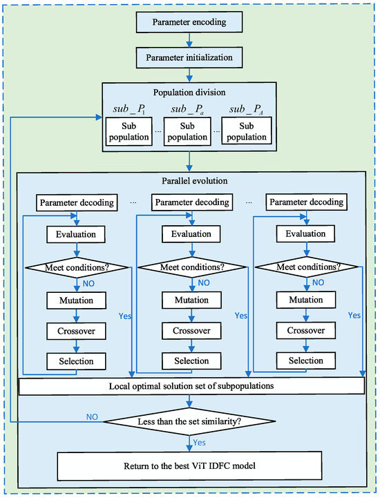
Figure 4. PDE algorithm flowchart.

4.2. LSTM-Based PDE Parameter Prediction Module

In the evolution process of PDE, the information of its $t\mathrm{th}$ generation population is determined from the 1st generation to the $(t-1)\mathrm{th}$ generation. Due to the randomness of ${\mathsf{\Theta }}_F^t$ and ${\mathsf{\Theta }}_{\mathrm{CR}}^t$, the evolutionary process of PDE can also be viewed as a random time series. Therefore, to adapt to its temporal dependence, an LSTM network is used here to obtain the ${\mathsf{\Theta }}_F^t$ and ${\mathsf{\Theta }}_{\mathrm{CR}}^t$ through online prediction.

Specifically, the fitness value $\mathrm{Fitness}(t)$ (denoted as $F^t$) of PDE and its statistical data $U^t$ are combined to form $A_t=[F^t,U^t]$ as the input for LSTM. Among them, $U^t$ is composed of the normalized histogram ${\dot{\mathit{f}}}_t$ and the moving average ${\overline{\mathit{f}}}_t$ of the histogram vectors from the past $g$ generation, denoted as $U^t=[{\dot{\mathit{f}}}_t,{\overline{\mathit{f}}}_t]$. The calculation process is shown below in detail.

Firstly, we normalize $F^t$ to obtain $\overline{f}$ as follows:

$$\overline{f}={\displaystyle \frac{f-\min \left\{F^t\right\}}{\max \left\{F^t\right\}-\min \left\{F^t\right\}}}$$

(17)

Then, we calculate the histogram ${\dot{\mathit{f}}}_t$ of $\overline{f}$ as follows:

$${\dot{\mathit{f}}}_t=histogram(\{\overline{f}\},b)$$

(18)

where $b$ is the number of bars in the histogram.

Furthermore, the moving average value ${\overline{\mathit{f}}}_t$ of the histogram vector of the previous generation $g$ is calculated as follows:

$${\overline{\mathit{f}}}_t={\displaystyle \frac{1}{g}}{\displaystyle \sum _{i=t-g}^{t-1}{\dot{\mathit{f}}}_i}$$

(19)

Finally, the input ${\mathit{A}}_t=[F^t,U^t]$ of the LSTM network is obtained to predict ${\mathsf{\Theta }}_t=[{\mathsf{\Theta }}_F^t,{\mathsf{\Theta }}_{\mathrm{CR}}^t]$.

The LSTM network introduces gate structures including forget gates, input gates, and output gates, as well as a memory unit to selectively receive information input into the neural network. The gate structure is responsible for connecting other parts of the neural network to the memory unit to complete weight setting.

Specifically, the forget gate receives information from the previous moment to the current moment, and calculates the degree of information retention $f_t$ based on the output $h_{t-1}$ from the previous moment and the input ${\mathit{A}}_t$ from the current moment as follows:

$$f_t=\sigma ({\mathit{W}}_f·[h_{t-1},{\mathit{A}}_t]+b_f)$$

(20)

where $\sigma$ is the sigmoid activation function.

The input gate first calculates its activation value $i_t$ based on $h_{t-1}$ and ${\mathit{A}}_t$, as follows:

$$i_t=\sigma ({\mathit{W}}_i·[h_{t-1},{\mathit{A}}_t]+b_i)$$

(21)

Next, we calculate the candidate values ${\tilde{C}}_t$ that may be added to the cell state as follows,

$${\tilde{C}}_t=\tanh ({\mathit{W}}_C·[h_{t-1},{\mathit{A}}_t]+b_C)$$

(22)

Then, based on the results of the first two steps, we calculate the updated unit status $C_t$ as follows,

$$C_t=f_t\otimes C_{t-1}+i_t\otimes {\tilde{C}}_t$$

(23)

where $\otimes$ represents Hadamard product.

The output gate calculates the degree of information output $o_t$ based on $h_{t-1}$ and ${\mathit{A}}_t$ as follows:

$$o_t=\sigma ({\mathit{W}}_o·[h_{t-1},{\mathit{A}}_t]+b_o)$$

(24)

The short-term memory value $h_t$ at the current time is obtained as follows:

$$h_t=o_t\otimes \tanh (C_t)$$

(25)

Finally, the current prediction result output by the network is as follows:

$${\widehat{\mathsf{\Theta }}}_t=\sigma ({\mathit{W}}^{\prime }{h}_t)$$

(26)

where ${\mathit{W}}^{\prime }$ is the output hidden layer weight.

Therefore, LSTM can be formalized as follows:

$$[{\widehat{\mathsf{\Theta }}}_t,C_t,h_t]=\mathrm{LSTM}({\mathit{A}}^t,h_{t-1},C_{t-1};\mathbf{W})$$

(27)

where $\mathbf{W}=[W_{f,}{W}_{i,}{W}_{c,}{W}_o,W^{\prime },b_f,b_i,b_c,b_o]$, $C_t$ represents long-term memory value, and $h_t$ represents short-term memory value.

The algorithm flowchart is shown in Figure 5.

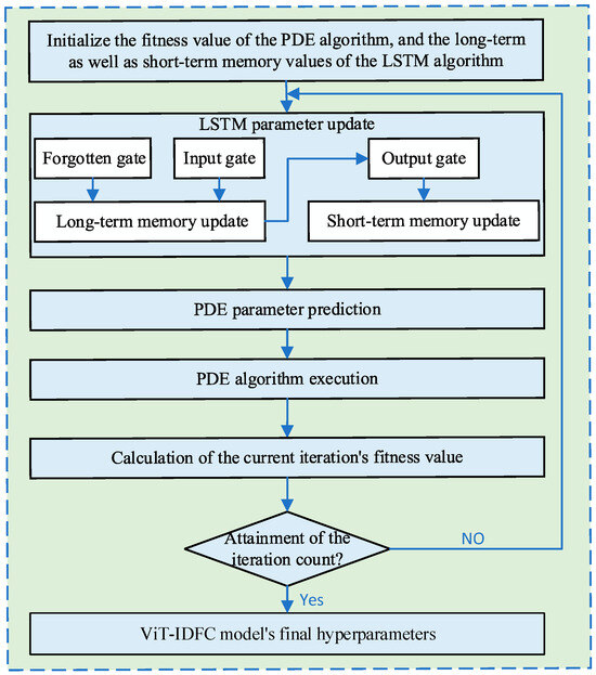
Figure 5. LSTM algorithm flowchart.

4.3. RL-Based LSTM Parameter Optimization Module

To optimize the evolutionary parameters of PDE, the LSTM used for PDE parameter prediction is first modeled as a Markov decision process (MDP). The definitions of environment, state, action, strategy, reward, and transfer are as follows.

(1)

Environment: Optimize the ViT-IDFC combustion state recognition model;

(2)

Status: Use fitness values $F^t$, statistics $U^t$, and short-term memory values $h^t$ as the status $s_t$;

(3)

Action: Define PDE parameters as actions, i.e., $a_t={\widehat{\mathsf{\Theta }}}_t=\{{\mathsf{\Theta }}_F^t,{\mathsf{\Theta }}_{\mathrm{CR}}^t\}$;

(4)

Strategy: Determined by LSTM parameters, as follows:

$$\pi (a_t|s_t)={\displaystyle \frac{1}{(2\pi {\sigma }^2)}}\exp \{-{\displaystyle \frac{1}{2{\sigma }^2}}{(a_t-LSTM(s_t;\mathbf{W}))}^2\}$$

(28)

(5)

Reward: Refers to the relative improvement of the best fitness value, as follows:

$$r_{t+1}={\displaystyle \frac{\max \left\{F^{t+1}\right\}-\max \left\{F^t\right\}}{\max \left\{F^t\right\}}}$$

(29)

(6)

Transition: Represented as a probability distribution $p(s_{t+1}|a_t,s_t)$. Here, the RL based variant algorithm Policy Gradient (PG) is used to handle the situation where the transition probability is unknown. The principle of this algorithm is to update policy parameters through random gradient ascent to maximize the expected value of rewards. In this way, algorithms can optimize the behavior of agents to adapt to unknown transition probability environments, as follows:

$$r_{t+1}=r_t+\alpha ·{\nabla }_{r}U(r_t)$$

(30)

where $\alpha$ represents the learning rate, and ${\nabla }_{r}U(r)$ represents the cumulative reward gradient.

For the proposed MDP, the joint probability of trajectory $\tau =\{s_0,a_0,r_1,\cdots ,a_{T-1},a_{T-1},r_T\}$ is as follows,

$$q(\tau ;r)=p(s_0){\displaystyle \prod _{t=0}^{T-1}\pi (a_t|s_t;r)p(s_{t+1}|a_t,s_t)}$$

(31)

Furthermore, the cumulative reward gradient ${\nabla }_{r}U(r)$ can be obtained as follows:

$$\begin{array}{ll}{\nabla }_{r}U(r)& ={\displaystyle \sum _{\tau }r(\tau )}{\nabla }_{r}q(\tau ;r)\\ & ={\displaystyle \sum _{\tau }r(\tau )}{\displaystyle \frac{{\nabla }_{r}q(\tau ;r)}{q(\tau ;r)}}q(\tau ;r)\\ & ={\displaystyle \sum _{\tau }r(\tau )}q(\tau ;r){\nabla }_{\theta }[\log q(\tau ;r)]\\ & ={\displaystyle \sum _{\tau }r(\tau )q(\tau ;r)}[{\displaystyle \sum _{t=0}^{T-1}{\nabla }_r\log \pi (a_t|s_t;r)}]\end{array}$$

(32)

where $r(\tau )$ is the cumulative reward of $\tau$.

The expected value of the above equation can be obtained through $L$ trajectory samples, as follows:

$$\nabla U_r(r)\approx {\displaystyle \frac{1}{L}}{\displaystyle \sum _{i=1}^{L}r({\tau }^i)}{\displaystyle \sum _{t=0}^{T-1}{\nabla }_r}\ln \pi (a_t^{(i)}|s_t^{(i)};r)$$

(33)

where $a_t^{(i)}$ represents the action value of the agent at time $t$ of the $i\mathrm{th}$ trajectory, and $s_t^{(i)}$ represents the state of the agent at time $t$ of the $i\mathrm{th}$ trajectory.

Therefore, according to Equation (29), it can be calculated to evaluate the actions $a_t$ taken by the agent in the current state $s_t$.

The algorithm flowchart is shown in Figure 6.

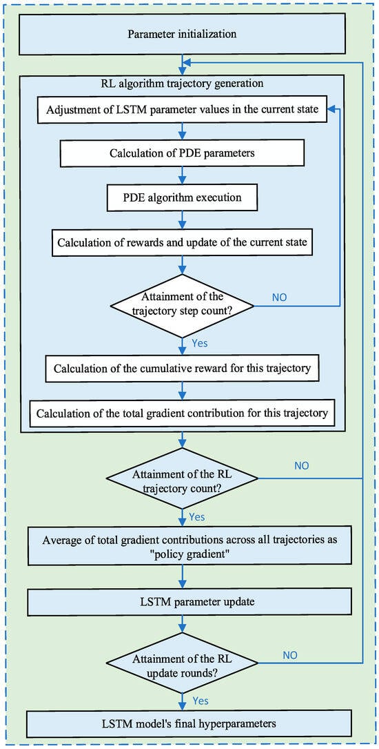
Figure 6. RL algorithm flowchart.

4.4. Pseudocode

Table 1 shows the pseudocode of the proposed algorithm.

Table 1. Pseudocode for flame combustion state recognition model based on deep feature and hyperparameter collaborative optimization.

Input: Original flame image dataset ${\{{\mathit{X}}_n^{\mathrm{Flame}},y_n^{\mathrm{Flame}}\}}_{n=1}^N$
Output: Flame image combustion state prediction output ${({\widehat{y}}_n^{\mathrm{Flame}})}_{n=1}^N$
Step1:	Randomly initialize the population of PDE $P^0$, initialize the long-term memory value $C^0=0$ and $h^0=0$ of LSTM
Step 2:	Set the iteration number Epoch = 1
Step 3:	Evaluate the fitness value of the population $F^0$, calculate fitness value statistic $U^0$, obtain input for LSTM $A^0=[U^0,F^0]$
Step 4:	Input $A^0$,$h^0$ and $C^0$ into the LSTM network
Step 5:	LSTM obtains the values of PDE parameters $F^0$ and $C{R}^0$ based on the optimization experience of trained agents
Step 6:	PDE optimizes the deep features and hyperparameters of the ViT-IDFC recognition model based on $F^0$ and $C{R}^0$
Step 7:	When the pre-set maximum iteration number of Epoch is reached, the process is stopped
Step 8:	Return the deep feature selection parameters ${[S_P^1, S_P^2, \cdots , S_P^{12}]}_{\mathrm{best}}$ and the model hyperparametersReturn the deep feature selection parameters that optimize the performance of the ViT-IDFC model, as well as the $M_{\mathrm{best}}$ and $J_{\mathrm{best}}$ hyperparameters of DFC
Step 9:	Construct the optimal recognition model

The proposed algorithm flowchart is shown in Figure 7.

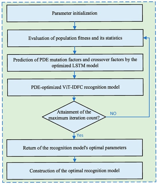
Figure 7. Algorithm flowchart.

5. Experimental Study

5.1. Hardware Configuration and Evaluation Indicators

The recognition model described in this article is built on Python 3.9 and Pytorch 1.12.0 GPU framework. The training and testing hardware environments are shown in Table 2.

Table 2. Hardware configuration.

Device	Configuration
System	Windows10
Memory	32 GB
GPU	Invidia GeForce RTX3060Ti
CPU	11th Gen Intel(R) Core(TM) i9-11900K

To evaluate the performance of the model, we used evaluation metrics such as confusion matrix, accuracy, precision, recall, F1-score and ROC-AUC. Table 3 shows the confusion matrix of the classification results, providing specific data for performance evaluation. Among them, TP represents the number of samples correctly predicted as positive by the model; FP denotes the number of samples incorrectly predicted as positive; TN indicates the number of samples correctly predicted as negative; and FN refers to the number of samples incorrectly predicted as negative.

Table 3. Classification result confusion matrix.

	Positive	Negative
Positive	TP (true positive)	FN (false negative)
Negative	FP (false positive)	TN (true negative)

Accuracy measures the proportion of correct predictions among all predictions made by the model, reflecting its overall performance; Precision measures the proportion of truly positive samples among those predicted as positive, indicating the accuracy of positive predictions; Recall measures the proportion of successfully predicted positive samples among all actual positive samples, reflecting the model’s ability to identify all relevant instances; F1-score reflects the model’s comprehensive performance in identifying positive-class samples, balancing both the accuracy of positive predictions and the coverage capability for positive instances; ROC-AUC indicates the model’s ability to distinguish between positive and negative samples across different classification thresholds. The value ranges of the above five metrics are all [0, 1], with higher values indicating better model performance. The definitions of Accuracy, Precision, Recall, F1-score and ROC-AUC are as follows.

$$\mathrm{Accuracy}={\displaystyle \frac{TP+TN}{TP+TN+FP+FN}}$$

(34)

$$\mathrm{Precision}={\displaystyle \frac{TP}{TP+FP}}$$

(35)

$$\mathrm{Recall}={\displaystyle \frac{TP}{TP+FN}}$$

(36)

$$\mathrm{F}1-\mathrm{score}={\displaystyle \frac{2\times TP}{2TP+FP+FN}}$$

(37)

$$\mathrm{FPR}={\displaystyle \frac{FP}{FP+TN}}$$

(38)

$$\mathrm{ROC}-\mathrm{AUC}={\displaystyle {\int }_0^1 \mathrm{Recall}(x)} d(\mathrm{FPR}(x))$$

(39)

5.2. Data Description

The flame image data used in this study was sourced from a MSWI power plant in Beijing. Due to the limited field of view of industrial cameras, one camera was installed at each end of the grate to capture flame videos.

We collected left and right single-channel flame videos from an MSWI power plant at a frame rate of 25 frames per second. Guided by expert experience, representative combustion state segments were then selected from the collected videos. The selected segment duration was 54 h and 49 min for the left grate and 44 h and 45 min for the right grate. These segments were sampled at a rate of one frame per minute to generate flame images. The specific distribution of the various typical combustion states is shown in Table 4, yielding 3289 images for the left grate and 2685 images for the right grate. These images cover flame states under multiple working conditions, including different waste input volumes, different grate speeds, and different air velocities, to ensure sample diversity and dataset representativeness. After randomly shuffling the dataset, it was split into training and testing sets in a 7:3 ratio.

Table 4. Flame image dataset.

Data Set	Total Number	Normal Burning	Partial Burning	Channeling Burning	Smoldering	Size
Left grate	3289	655	1176	1044	414	720 × 576
Right grate	2685	564	1002	534	585	720 × 576

Remark 1. 

The composition of waste shows significant variability due to residents’ living habits and seasonal consumption patterns. During combustion, water evaporation results in relatively low flame temperatures, which typically appear as low-brightness features in images. In contrast, dry waste produces higher image brightness and more dynamic flame contours. This variability in the dataset directly impacts the feature extraction logic of the model, affecting recognition stability across different scenarios. To mitigate the impact of such variability on the model’s generalization capability, future research will expand the dataset coverage to ensure a comprehensive sample distribution that accounts for fluctuations in seasonal waste composition and environmental conditions.

5.3. Experimental Result

5.3.1. Deep Features and Hyperparameter Selection Results

Table 5 shows the deep features and hyperparameter optimization results of ViT-IDFC based on PDE.

Table 5. Hyperparameter optimization results.

Grate	Before and After Optimization	Parameter Settings
		$[{\mathit{S}}_{\mathit{P}}^1, {\mathit{S}}_{\mathit{P}}^2, \cdots , {\mathit{S}}_{\mathit{P}}^{12}]$	$\mathit{J}$	$\mathit{M}$
Left	Before optimization	[0, 0, 1, 1, 1, 1, 1, 1, 1, 1, 1, 1]	50	3
	After optimization	[1, 1, 0, 1, 0, 1, 0, 1, 1, 0, 0, 1]	100	1
Right	Before optimization	[0, 0, 0, 0, 0, 0, 1, 1, 1, 1, 1, 1]	50	3
	After optimization	[0, 0, 0, 0, 1, 1, 1, 1, 0, 1, 1, 1]	100	1

According to Table 5, after PDE optimization, both the feature selection parameters and model hyperparameters of the left and right grate recognition models have undergone changes. Among them, the feature selection parameters for both grates have selected 7 layers of deep features as input to the recognition model. However, the specific deep feature layers selected differ between the left and right grates, which is related to the distribution differences in the flame images from the two grates.

5.3.2. PDE Parameter Optimization Results

The optimization results of PDE parameters based on LSTM network are shown in Figure 8.

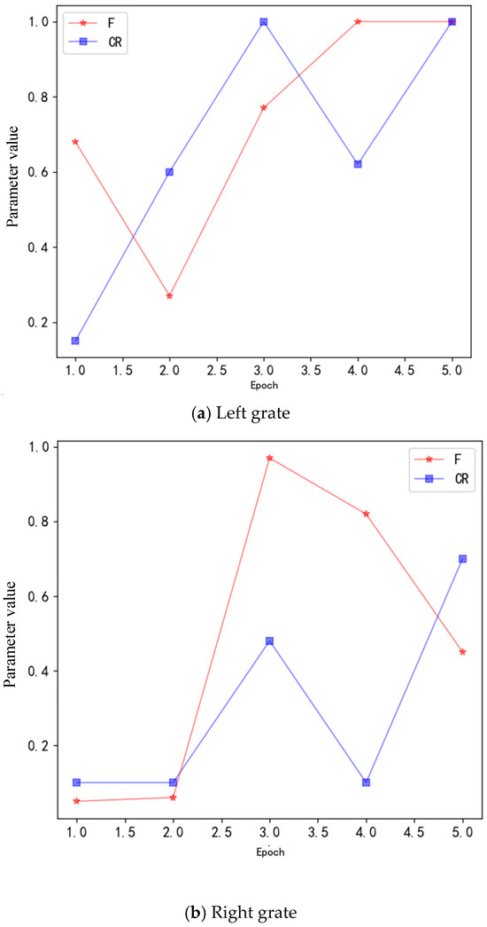
Figure 8. PDE parameter optimization results.

As shown in Figure 8, during the optimization process of PDE mutation factor and crossover factor based on LSTM network, F and CR gradually approach 1 in the optimization process of the left grate recognition model, while F and CR gradually approach 0.5 in the optimization process of the right grate recognition model. In the process of learning LSTM parameters based on RL, the reward value of RL is consistent with the accuracy value of the model and shows an increasing trend. This indicates that the agent gradually masters the experience of making the recognition model achieve the best performance during the learning process, and ultimately achieves the best recognition performance through parameter optimization.

5.3.3. Optimize Model Recognition Results

Table 6 shows the recognition results of the optimized model before and after deep feature and hyperparameter optimization.

Table 6. Results of hyperparameter optimization.

Grate	Before and After Optimization	Evaluation Indicators
		Accuracy	Precision	Recall	F1-Score	ROC-AUC
Left	Before optimization	0.9289	0.9351	0.9225	0.9284	0.9925
	After optimization	0.9340	0.9389	0.9283	0.9333	0.9931
Right	Before optimization	0.9030	0.9120	0.8961	0.9027	0.9870
	After optimization	0.9104	0.9169	0.9032	0.9092	0.9879

As shown in Table 6, the RL-LSTM-PDE optimization algorithm has improved the recognition performance for both the left and right grate models through multi-level optimization based on the integration of RL, LSTM, and PDE. Specifically, the recognition accuracy increased by 0.51% for the left grate and 0.74% for the right grate.

The trend of RL reward value and recognition model accuracy value changing with epoch is shown in.

As shown in Figure 9, during the process of learning LSTM parameters based on RL, the reward value of RL is consistent with the accuracy value of the model and shows an increasing trend. This indicates that the agent gradually obtains the experience of achieving the optimal recognition effect of the model during the learning process, and ultimately achieves the best recognition effect through parameter optimization.

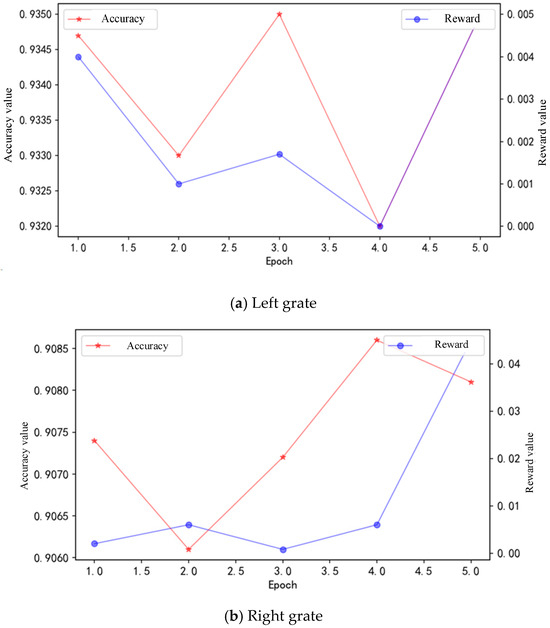
Figure 9. Relation between values of RL reward and recognition model accuracy and learning epoch.

Figure 10 shows the confusion matrix of the optimized left/right grate recognition results.

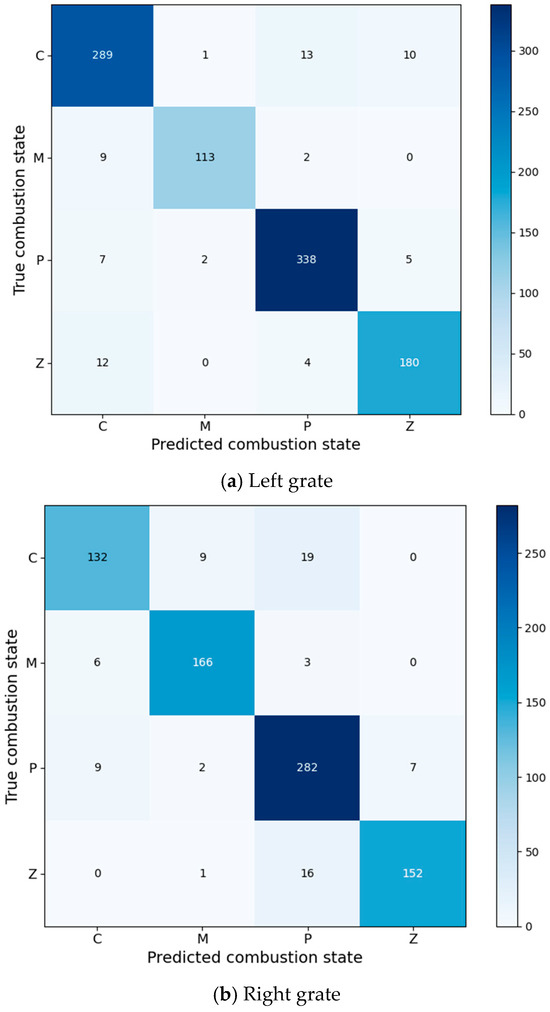
Figure 10. Confusion matrix of model recognition results.

In the matrix shown in Figure 10, C, M, P, and Z represent the four flame combustion states: Channeling burning, Smoldering, Partial burning, and Normal burning, respectively. The rows of the matrix correspond to the predicted combustion states, while the columns represent the true combustion states by the model.

The numbers along the diagonal indicate the count of correctly predicted samples. For example, the value in the first row and first column represents the number of samples correctly predicted as Channeling burning. The off-diagonal elements represent misclassified samples. For instance, the value in the first row and second column indicates the number of samples where Channeling burning was incorrectly predicted as Smoldering. The misclassification count for each combustion state is calculated by summing the off-diagonal elements in each row of the matrix. The optimal combustion state is determined as the category with the highest diagonal value and the lowest misclassification count.

From Figure 10, the combustion categories of both the left and right grate are prone to misidentification. This is because the combustion state often occurs in the transition stage of other combustion states, and therefore the flame image features are coupled with other categories. The Partial burning state is the least prone to misidentification, as its flame image features are relatively simple and differ significantly from other states.

5.3.4. Computational Complexity Analysis

The computational complexity of a single forward pass of the ViT-IDFC model is $O(mode{l}_{\mathrm{ViT}-\mathrm{IDFC}})$; the computational complexity of the PDE algorithm is $O({\mathsf{\Theta }}_{\mathrm{PDE}}\times NP\times mode{l}_{\mathrm{ViT}-\mathrm{IDFC}})$; the computational complexity of the LSTM model is $O({\mathsf{\Theta }}_{\mathrm{PDE}}\times H^2)$, where $H$ is the size of the hidden layer; and the computational complexity of RL is $O(L\times {\mathsf{\Theta }}_{\mathrm{PDE}}\times NP\times mode{l}_{\mathrm{ViT}-\mathrm{IDFC}})$.

During the training phase, the computational complexity of the LSTM model is significantly lower than that of RL and can be neglected. Therefore, the overall computational complexity of the proposed RL-LSTM-PDE method is denoted $O(L\times {\mathsf{\Theta }}_{\mathrm{PDE}}\times NP\times mode{l}_{\mathrm{ViT}-\mathrm{IDFC}})$. During the inference phase, the time cost is completely decoupled from the optimization framework and is equivalent to the computational cost of a single ViT-IDFC model, denoted as $O(mode{l}_{\mathrm{ViT}-\mathrm{IDFC}})$.

Under the standard hardware configuration specified in Table 2, tests conducted on the left grate model demonstrated that completing the ViT-IDFC parameter optimization required approximately 4.2 h when the training epoch was set to 5. During this process, hardware resources were dedicated to core computational tasks including feature extraction, LSTM parameter inference, and PDE population optimization, with no redundant computations. This resource allocation aligns with the conventional load capacity of such hardware systems.

5.4. Method Comparison

To verify the superiority of the proposed method, it was compared with some other methods. The parameter settings are shown in Table 7, and the recognition results of the left/right grate flame images are shown in Table 8 and Table 9.

Table 7. Parameter setting statistics of comparison methods.

Method	(Sub) Population Size	Sub Population Number	Epoch	Trajectory Length	Trajectory Number
DE	5	-	5	-	-
PDE	5	3	35	-	-
RL-LSTM-DE	5	3	5	3	5
This study	10	2	5	2	3

Table 8. Comparative experimental results of left grate flame image models.

Method	Parameter Settings			Accuracy	Precision	Recall	F1-Score	ROC-AUC
	${({\mathit{X}}_{\mathbf{ViT}}^{\mathit{k}})}_{\mathit{k}=1}^{12}$	$\mathit{J}$	$\mathit{M}$
DE	[0, 0, 0, 0, 0, 1, 0, 0, 0, 0, 1, 0]	43	5	0.9127	0.9195	0.9036	0.9109	0.9891
PDE	[0, 1, 0, 1, 0, 1, 0, 1, 1, 0, 1, 0]	51	1	0.9289	0.9319	0.9236	0.9276	0.9929
RL-LSTM-DE	[1, 1, 1, 1, 1, 0, 0, 1, 0, 0, 0, 1]	90	5	0.9188	0.9240	0.9106	0.9168	0.9905
This study	[1, 1, 0, 1, 0, 1, 0, 1, 1, 0, 0, 1]	100	1	0.9340	0.9389	0.9283	0.9333	0.9931

Table 9. Comparative experimental results of right grate flame image models.

Method	Parameter Settings			Accuracy	Precision	Recall	F1-Score	ROC-AUC
	${({\mathit{X}}_{\mathbf{ViT}}^{\mathit{k}})}_{\mathit{k}=1}^{12}$	$\mathit{J}$	$\mathit{M}$
DE	[1, 0, 0, 0, 1, 1, 1, 0, 0, 0, 0, 1]	37	1	0.8806	0.8888	0.8682	0.8750	0.9819
PDE	[0, 0, 0, 0, 0, 0, 1, 0, 1, 1, 1, 1]	39	1	0.9005	0.9085	0.8906	0.8970	0.9848
RL-LSTM-DE	[1, 1, 1, 1, 1, 1, 0, 0, 0, 1, 1, 0]	27	2	0.8868	0.8931	0.8775	0.8835	0.9838
This study	[0, 0, 0, 0, 1, 1, 1, 1, 0, 1, 1, 1]	100	1	0.9104	0.9169	0.9032	0.9092	0.9879

According to Table 8 and Table 9, compared to other methods, the method proposed in this article has the best optimization effect on the recognition model. The multi-level collaborative optimization architecture adopted in the proposed method achieves a three-layer interaction among RL, LSTM, and PDE. RL globally guides the optimization direction through a reward mechanism; LSTM dynamically interprets the optimization status and finely adjusts the hyperparameters of PDE; and PDE collaboratively explores the solution space with multiple subpopulations. This deeply coupled mechanism significantly enhances global optimization capability and model expressiveness, leading to comprehensive performance that surpasses compared models. Furthermore, the proposed method employs a parallel differential evolution framework, which significantly enhances operational efficiency compared to the RL-LSTM-DE approach. However, due to the incorporation of RL-LSTM networks for parameter prediction and optimization, the computational complexity of the proposed method is higher than that of conventional DE and PDE algorithms. Despite this increased complexity, the method achieves a substantial improvement in recognition accuracy. These results demonstrate that the proposed approach strikes an effective balance between computational efficiency and model performance.

5.5. Ablation Experiment

Table 10 and Table 11 present the ablation experimental results of the RL-LSTM-PDE method proposed in this study, based on the left and right grate flame images, respectively.

Table 10. Experimental results of left grate ablation.

Method	Parameter Settings			Accuracy	Precision	Recall	F1-Score	ROC-AUC
	${({\mathit{X}}_{\mathbf{ViT}}^{\mathit{k}})}_{\mathit{k}=1}^{12}$	$\mathit{J}$	$\mathit{M}$
PDE	[0, 1, 0, 1, 0, 10, 1, 1, 0, 1, 0]	51	1	0.9289	0.9319	0.9236	0.9276	0.9929
LSTM-PDE	[0, 0, 1, 1, 0, 1, 1, 0, 1, 0, 1, 1]	55	1	0.9299	0.9399	0.9183	0.9277	0.9915
RL-LSTM-PDE	[1, 1, 0, 1, 0, 1, 0, 1, 1, 0, 0, 1]	100	1	0.9340	0.9389	0.9283	0.9333	0.9931

Table 11. Results of right grate ablation experiment.

Method	Parameter Settings			Accuracy	Precision	Recall	F1-Score	ROC-AUC
	${({\mathit{X}}_{\mathbf{ViT}}^{\mathit{k}})}_{\mathit{k}=1}^{12}$	$\mathit{J}$	$\mathit{M}$
PDE	[0, 0, 0, 0, 0, 0, 1, 0, 1, 1, 1, 1]	39	1	0.9005	0.9085	0.8906	0.8970	0.9848
LSTM-PDE	[1, 1, 0, 1, 1, 1, 1, 1, 0, 1, 1, 1]	21	1	0.9030	0.9092	0.8949	0.9009	0.9869
RL-LSTM-PDE	[0, 0, 0, 0, 1, 1, 1, 1, 0, 1, 1, 1]	100	1	0.9104	0.9169	0.9032	0.9092	0.9879

According to Table 10 and Table 11, when optimizing the recognition model parameters based on PDE and LSTM-PDE algorithms, the performance improvement is very limited, and even the model performance decreases, indicating that its global search ability is still very limited. When optimizing the recognition model based on the proposed RL-LSTM-PDE algorithm, the model performance can reach its optimal level.

6. Conclusions

To address the challenges of time consumption, high dependency, and difficulty in adaptively achieving optimal results when manually selecting optimization features and hyperparameters based on experience for the MSWI flame combustion state recognition model, an optimization method for collaboratively optimizing deep features and model hyperparameters is proposed. The optimization framework of the proposed method is essentially a general-purpose adaptive model optimizer, whose design is independent of the inherent characteristics of any specific species or dataset. By replacing the target dataset and correspondingly adjusting the preprocessing parameters of the model’s input layer, the framework can be quickly adapted to a variety of application scenarios, such as plant species recognition and combustion state classification in coal-fired power plants, demonstrating its capability for cross-scene migration and adaptation.

The main contributions of this study are as follows: (1) proposing a deep feature and hyperparameter optimization strategy for the recognition model based on RL-LSTM-PDE, which reduces the time-consuming process and inconsistencies caused by reliance on manual experience for feature and hyperparameter selection; (2) transforming the deep feature selection and hyperparameter optimization problem of the combustion state recognition model into a coding design and optimization problem for the PDE algorithm, reinterpreting the determination of mutation and selection factors for the PDE algorithm as an LSTM model prediction task, and framing the optimization of LSTM parameters as an RL problem within the context of optimizing the ViT-IDFC combustion state recognition model; (3) implementing the optimization of deep features and model hyperparameters for the ViT-IDFC combustion state recognition model based on the proposed strategy, and validating its effectiveness using real process data.

In the field of industrial AI applications, the integration of interpretable AI methods has become a crucial component for building trustworthy systems. The ViT-IDFC model used in this article not only visually identifies the key regions of flame images with varying depth features but also demonstrates intrinsic recognition causality through a decision tree-based recognition algorithm that offers traceability and interpretability. These features make the inference process of complex models transparent and traceable, helping operators understand the decision logic behind AI. This transparency is critical in enhancing the reliability of human–machine collaboration, particularly in industrial environments.

Future research should focus on reducing the time cost associated with the operation of this strategy. Additionally, we will collect flame image data under various operating conditions from multiple MSWI facilities and validate the methodology through extendable testing.

References

- Gómez-Sanabria, A.; Kiesewetter, G.; Klimont, Z.; Schoepp, W.; Haberl, H. Potential for future reductions of global GHG and air pollutants from circular waste management systems. Nat. Commun. 2022, 13, 106. [Google Scholar] [CrossRef]
- Ali, K.; Kausar, N.; Amir, M. Impact of pollution prevention strategies on environment sustainability: Role of environmental management accounting and environmental proactivity. Environ. Sci. Pollut. Res. 2023, 30, 88891–88904. [Google Scholar] [CrossRef]
- Tang, J.; Xia, H.; Yu, W.; Qiao, J.F. Research status and prospects of intelligent optimization control for municipal solid waste incineration process. Acta Autom. Sin. 2023, 49, 2019–2059. [Google Scholar]
- Song, Y.; Xian, X.; Zhang, C.; Zhu, F.; Yu, B.; Liu, J. Residual municipal solid waste to energy under carbon neutrality: Challenges and perspectives for China. Resour. Conserv. Recycl. 2023, 198, 107177. [Google Scholar] [CrossRef]
- Tang, L.; Guo, J.; Wan, R.; Jia, M.; Qu, J.; Li, L.; Bo, X. Air pollutant emissions and reduction potentials from municipal solid waste incineration in China. Environ. Pollut. 2023, 319, 121021. [Google Scholar] [CrossRef] [PubMed]
- Walser, T.; Limbach, L.K.; Brogioli, R.; Erismann, E.; Flamigni, L.; Hattendorf, B.; Juchli, M.; Krumeich, F.; Ludwig, C.; Prikopsky, K.; et al. Persistence of engineered nanoparticles in a municipal solid-waste incineration plant. Nat. Nanotechnol. 2012, 7, 520–524. [Google Scholar] [CrossRef] [PubMed]
- Istrate, I.R.; Galvez-Martos, J.L.; Vázquez, D.; Guillén-Gosálbez, G.; Dufour, J. Prospective analysis of the optimal capacity, economics and carbon footprint of energy recovery from municipal solid waste incineration. Resour. Conserv. Recycl. 2023, 193, 106943. [Google Scholar] [CrossRef]
- Fernando, Y.; Tseng, M.L.; Aziz, N.; Ikhsan, R.B.; Wahyuni-TD, I.S. Waste-to-energy supply chain management on circular economy capability: An empirical study. Sustain. Prod. Consum. 2022, 31, 26–38. [Google Scholar] [CrossRef]
- Kalyani, K.A.; Pandey, K.K. Waste to energy status in India: A short review. Renew. Sustain. Energy Rev. 2014, 31, 113–120. [Google Scholar] [CrossRef]
- Liu, J.; Hu, L.; Tang, L.; Ren, J. Utilisation of municipal solid waste incinerator (MSWI) fly ash with metakaolin for preparation of alkali-activated cementitious material. J. Hazard. Mater. 2021, 402, 123451. [Google Scholar] [CrossRef]
- Fan, C.; Wang, B.; Qi, Y.; Liu, Z. Characteristics and leaching behavior of MSWI fly ash in novel solidification/stabilization binders. Waste Manag. 2021, 131, 277–285. [Google Scholar] [CrossRef]
- Song, L.; Sun, Y.; Song, J.; Feng, Z.; Gao, J.; Yao, Q. From “not in my backyard” to “please in my backyard”: Transforming the local responses toward a waste-to-energy incineration project in China. Sustain. Prod. Consum. 2024, 45, 104–114. [Google Scholar] [CrossRef]
- Liang, X.; Kurniawan, T.A.; Goh, H.H.; Zhang, D.; Dai, W.; Liu, H.; Goh, K.C.; Othman, M.H.D. Conversion of landfilled waste-to-electricity (WTE) for energy efficiency improvement in Shenzhen (China): A strategy to contribute to resource recovery of unused methane for generating renewable energy on-site. J. Clean. Prod. 2022, 369, 133078. [Google Scholar] [CrossRef]
- Liang, D.; Wang, F.; Lv, G. The resource utilization and environmental assessment of MSWI fly ash with solidification and stabilization: A review. Waste Biomass Valorization 2024, 15, 37–56. [Google Scholar] [CrossRef]
- Cao, C.; Zhang, Q.; Li, M.H.; Wang, S.Y. Flame combustion state recognition in municipal solid waste incineration processes based on image multi-threshold segmentation and DQN-PL model. Energy 2025, 331, 136967. [Google Scholar] [CrossRef]
- Zhou, C.; Cao, Y.; Yang, S. Video Based Combustion State Identification for Municipal Solid Waste Incineration. IFAC-Pap. 2020, 53, 13448–13453. [Google Scholar] [CrossRef]
- Huang, S. Research on the Diagnosis Method of Large scale Household Waste Incineration Process Based on Machine Vision. Zhejiang University: Hangzhou, China, 2020. [Google Scholar]
- Zhou, Z.C. Research on Combustion State Diagnosis of Garbage Incinerator Based on Image Processing and Artificial Intelligence. Southeast University: Nanjing, China, 2015. [Google Scholar]
- Qiao, J.F.; Duan, H.S.; Tang, J.; Meng, X. MSWI combustion condition recognition based on flame image color features. Control Eng. 2022, 29, 1153–1161. [Google Scholar]
- Guo, H.T.; Tang, J.; Ding, H.X.; Qiao, J.F. Combustion states recognition method of MSWI process based on mixed data enhancement. Acta Autom. Sin. 2024, 50, 560–575. [Google Scholar]
- Pan, X.T.; Tang, J.; Xia, H.; Yu, W.; Qiao, J.F. Combustion state identification of MSWI processes using ViT-IDFC. Eng. Appl. Artif. Intell. 2023, 126, 106893. [Google Scholar] [CrossRef]
- Bian, C.; Zhou, Y.W.; Li, M.Q.; Qian, C. Stochastic population update can provably be helpful in multi-objective evolutionary algorithms. Artif. Intell. 2025, 341, 104308. [Google Scholar] [CrossRef]
- Singh, D.; Kaur, M.; Jabarulla, M.Y.; Kumar, V.; Lee, H. Evolving fusion-based visibility restoration model for hazy remote sensing images using dynamic differential evolution. IEEE Trans. Geosci. Remote Sens. 2022, 60, 1–14. [Google Scholar] [CrossRef]
- Singh, D.; Kumar, V.; Vaishali; Kaur, M. Classification of COVID-19 patients from chest CT images using multi-objective differential evolution–based convolutional neural networks. Eur. J. Clin. Microbiol. Infect. Dis. 2020, 39, 1379–1389. [Google Scholar] [CrossRef]
- Chen, X.; Shen, A. Self-adaptive differential evolution with Gaussian–Cauchy mutation for large-scale CHP economic dispatch problem. Neural Comput. Appl. 2022, 34, 11769–11787. [Google Scholar] [CrossRef]
- Liang, X.X.; Feng, Y.H.; Ma, Y.; Cheng, G.Q.; Huang, J.C.; Wang, Q.; Zhou, Y.Z. Deep multi-agent reinforcement learning: A survey. Acta Autom. Sin. 2020, 46, 2537–2557. [Google Scholar]
- Zhou, P.; Wang, X.; Chai, T. Multiobjective operation optimization of wastewater treatment process based on reinforcement self-learning and knowledge guidance. IEEE Trans. Cybern. 2022, 53, 6896–6909. [Google Scholar] [CrossRef]
- Pan, Z.X.; Wang, L.; Wang, J.J.; Lu, J.W. Deep reinforcement learning based optimization algorithm for permutation flow-shop scheduling. IEEE Trans. Emerg. Top. Comput. Intell. 2021, 7, 983–994. [Google Scholar] [CrossRef]
- Tian, Y.; Li, X.P.; Ma, H.P.; Zhang, X.Y.; Tian, K.C.; Jin, Y.C. Deep reinforcement learning based adaptive operator selection for evolutionary multi-objective optimization. IEEE Trans. Emerg. Top. Comput. Intell. 2022, 7, 1051–1064. [Google Scholar] [CrossRef]
- Hu, Z.; Gong, W.; Li, S. Reinforcement learning-based differential evolution for parameters extraction of photovoltaic models. Energy Rep. 2021, 7, 916–928. [Google Scholar] [CrossRef]
- Tan, Z.P.; Li, K.S. Differential evolution with mixed mutation strategy based on deep reinforcement learning. Appl. Soft Comput. 2021, 111, 107678. [Google Scholar] [CrossRef]
- Sun, J.; Liu, X.; Bäck, T.; Xu, Z. Learning Adaptive Differential Evolution Algorithm From Optimization Experiences by Policy Gradient. IEEE Trans. Evol. Comput. 2021, 25, 666–680. [Google Scholar] [CrossRef]
- Li, T.L.; Li, Y.F.; Wang, F.; Gong, C.; Zhang, J.R.; Ma, H. Improved parallel differential evolution algorithm with small population for multi-period optimal dispatch problem of microgrids. Energies 2025, 18, 3852. [Google Scholar] [CrossRef]
Disclaimer/Publisher’s Note: The statements, opinions and data contained in all publications are solely those of the individual author(s) and contributor(s) and not of MDPI and/or the editor(s). MDPI and/or the editor(s) disclaim responsibility for any injury to people or property resulting from any ideas, methods, instructions or products referred to in the content. |
© 2025 by the authors. Licensee MDPI, Basel, Switzerland. This article is an open access article distributed under the terms and conditions of the Creative Commons Attribution (CC BY) license (https://creativecommons.org/licenses/by/4.0/).