Analysis of the Summer Sea Breeze Cooling Capacity on Coastal Cities Based on Computer Fluid Dynamics

Abstract

Summer sea breezes provide cooling in coastal cities; however, their temporal cooling distribution and inland penetration distance remain inadequately studied. This study employed the mesoscale Weather Research and Forecasting (WRF) model to analyze the sea breeze cooling capacity (SBCC) in detail. The results identified the distance from the coast, cooling timing, and proximity to inland rivers as key factors influencing the SBCC. The cooling range and intensity of sea breezes exhibited a temporal pattern, initially increasing and then decreasing, with the rate of increase significantly exceeding the decline. The maximum cooling range (277.44 km²) and strongest cooling intensity (37,989.61 °C.h) occurred at 10:00. Between 11:00 and 14:00, the cooling effect remained stable over its longest inland distance (16.2 km). The SBCC intensified notably closer to the coastline. Furthermore, inland rivers significantly enhanced the cooling effect, with the sea breeze penetration distance correlating positively with the proximity to these rivers. A detailed analysis of the SBCC’s spatial extent and cooling distance provides a crucial basis for effectively mitigating urban heat in coastal cities.

1. Introduction

Owing to global warming, cities worldwide have been affected by heat waves. The Intergovernmental Panel on Climate Change has noted that heat waves will increase in their frequency and duration [1,2], which has attracted increasing scholarly attention. Heat waves have an impact on human health [3,4], the economy [5], and infrastructure [6]; the natural environment contributes to adverse impacts, and there is a strong relationship between heat waves and human mortality [7,8,9]. The problem of heat waves in large cities is exacerbated by factors such as the urban structure, urban land cover, underlying surfaces in cities, and building materials [10].

The phenomenon in which urban areas are warmer than the surrounding suburbs is called an urban heat island [11,12], which is closely related to the urban size and population density [13]. In the process of rapid urbanization, humans change the land use and cover, which leads to a decrease in the wind speed, vegetation, and permeable surface coverage, an increase in the use of high-thermal-mass materials, and an increase in an anthropogenic heat release in urban areas, thus aggravating the urban heat island effect [14]. Most cities worldwide are affected by urban heat islands to varying degrees [15,16,17,18,19]; they adversely affect ecosystems [20] and uncomfortable outdoor environments increase the water [21] and electricity [22] consumption, particularly during summer months [23,24]. Therefore, the reduction in the harmful effects of urban heat islands is an urgent challenge for cities.

Owing to the ease of maritime transport, most of the world’s economic activity occurs in coastal cities, resulting in over 50% of the global population living in urban areas within 200 km of a coastline [25]. As the population of coastal cities increases, urban areas expand faster, further exacerbating the urban heat island effect. The thermal risk index of coastal cities is significantly higher than that of inland cities [26]. Owing to different thermal characteristics, the difference in the air temperature between land and sea creates a horizontal pressure difference that allows shallow marine air to move inland, thus creating sea breezes, which typically occur during the day when the land surface heats faster than the ocean [27,28,29]. Sea breezes are mesoscale atmospheric phenomena that occur in coastal cities and recur over approximately two-thirds of the world’s coastlines [30]. The interaction between urban environments and sea breezes affects the climate system of coastal urban areas [31,32,33], thereby changing the climate inside cities [34,35,36]. Sea breeze fronts (the boundary between the advancing sea breeze and the warmer inland air) transport cool air to urban areas [37,38,39]. This important ventilation mechanism can effectively reduce the urban heat island intensity in coastal cities [40,41,42,43,44]. Therefore, it is of great significance for coastal cities to use sea breezes to alleviate urban thermal effects. Extensive research confirms that sea breezes mitigate urban heat islands in coastal areas [45,46,47,48,49]. Some studies have confirmed the impact of sea breeze on the temperature inside cities. Kolokotsa et al. [50] found that when sea breeze flows into the city, the temperature can be reduced to 26 °C, 4 °C lower than that in the case of no wind. Papanastasiou et al. [51] confirmed that sea breezes caused temperatures inside Greek cities to drop by at least 4 °C.

Research indicates that multiple factors modulate the cooling effect of sea breezes in coastal cities, encompassing both urban and natural features. Regarding urban form, the structural configuration of cities alters sea breeze circulation patterns [52,53,54]. Specifically, high-rise development increases the surface roughness, diminishing the sea breeze intensity and effectiveness [34,35,55,56,57] and lowering the average wind speeds [58]. Natural features also significantly influence cooling: the coastal morphology and proximity, alongside internal elements like rivers and forests, impact sea breeze penetration. Studies confirm that the coastline shape governs the sea breeze strength [59], while the distance from the coast serves as a key predictor for the urban heat island intensity [60]. This cooling capacity attenuates with the distance from the shoreline and, as Al-Ruzouq et al. [61] (focused on arid region coastal cities) noted, coastal areas may exhibit surface temperatures ~9 °C lower than inland zones—this discrepancy is context-dependent, modulated by arid climates (an intensified land–sea thermal contrast via strong solar radiation), distinct land cover, a gentle topography (aiding sea breeze penetration), and temporal variability (peaking at high solar radiation). Furthermore, the topography dictates the timing of sea breeze onset [62] and critically shapes the evolution of its circulation patterns [63]. However, the amount of cooling generated by sea breezes in coastal cities remains unknown. Additionally, the distribution of the cooling capacity and cooling range over time have remained largely unquantified, with only a few studies having been conducted on this topic.

At present, a numerical simulation is the main method for studying sea breezes, typically using mesoscale (10–100 km) models such as the Weather Research and Forecasting (WRF) model. Hai et al. [64] simulated the WRF model and concluded that the urban heat island effect would strengthen the sea breeze and increase the land–sea temperature difference. Kitao et al. [65] calculated the average wind speed per 1 km grid in summer based on the numerical simulation results of the wind speed of the WRF model. He et al. [66] used the WRF model to simulate typical sea and land winds in Shanghai. Validation against observational data from five weather stations confirmed the WRF model’s capability to reproduce temporal variations in meteorological variables during sea–land breeze cycles. Advances in computing technology have enabled an enhanced WRF model resolution and expanded computational fluid dynamics (CFD) domain sizes [67,68,69], achieving spatial alignment between the CFD simulation domain and the WRF model’s minimum grid scale.

The primary objective of this study is to quantitatively analyze the spatiotemporal characteristics of the Sea Breeze Cooling Capacity (SBCC)—including its hourly variation, inland penetration distance, and spatial extent—in the coastal city of Sendai, Japan, using the Weather Research and Forecasting (WRF) model. We aim to generate a detailed cooling map of the SBCC and dynamically analyze its trends. Furthermore, this research seeks to elucidate the key factors modulating the SBCC, such as proximity to the coastline, the timing of the cooling effect, and the influence of inland rivers. By providing a refined analysis of the SBCC’s spatial distribution and cooling penetration, this study intends to contribute a crucial scientific basis for urban planning strategies designed to harness natural ventilation and effectively mitigate urban heat island effects in coastal cities.

2. Data and Methods

2.1. Study Area

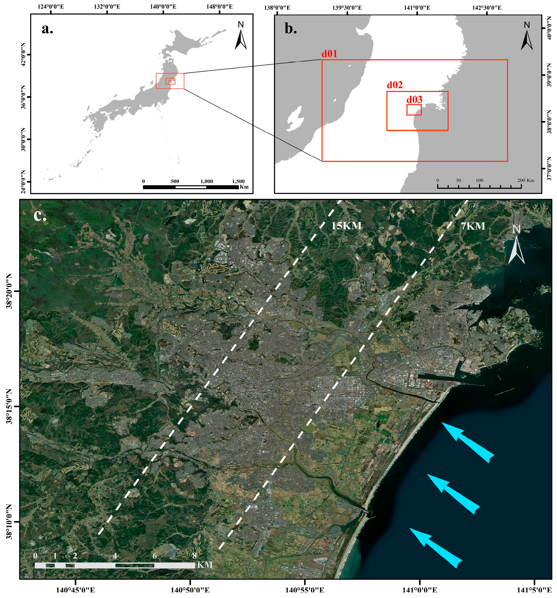
As the capital of Miyagi Prefecture and Tohoku’s largest urban center, Sendai lies on the Pacific coast with a subtropical monsoonal climate. The city’s topography consists of plains in the southeast, mountains in the northwest, and a central hilly terrain, covering a total area of approximately 785.8 km² (Figure 1). Sendai’s metropolitan zone extends about 40 km from the southeastern coast northwestward. Like many coastal cities with mountainous interiors, its developed areas are concentrated near the shoreline, placing the urban core merely 9 km from the coast. Statistical data indicate that Sendai’s mean annual temperature is increasing at 2.3 °C per century [70]. Research indicates that summer sea breezes effectively mitigate rising temperatures in Sendai [71]. Investigating this urban cooling mechanism could, therefore, contribute to developing strategies against warming trends.

Figure 1. Geographic extent and numerical modeling grid. (a) Map of Japan; (b) nested domains; (c) satellite view of Domain 3, showing the coastal zone (0–7 km), urban zone (7–15 km), and inland zone (>15 km). Arrows indicate the direction of the sea breeze.

2.2. Data

In this study, days with southeast and west winds were defined as “sea breeze days” and “west wind days”, respectively. The specific identification methods and conditions are explained in Section 2.3. To identify a “sea breeze day” and “west wind day” and select the target day for calculation and research, this study uses weather station data, multi-point observation data of the laboratory over a long period, and WRF model calculation data. The above data were used as follows.

2.2.1. Weather Station Data

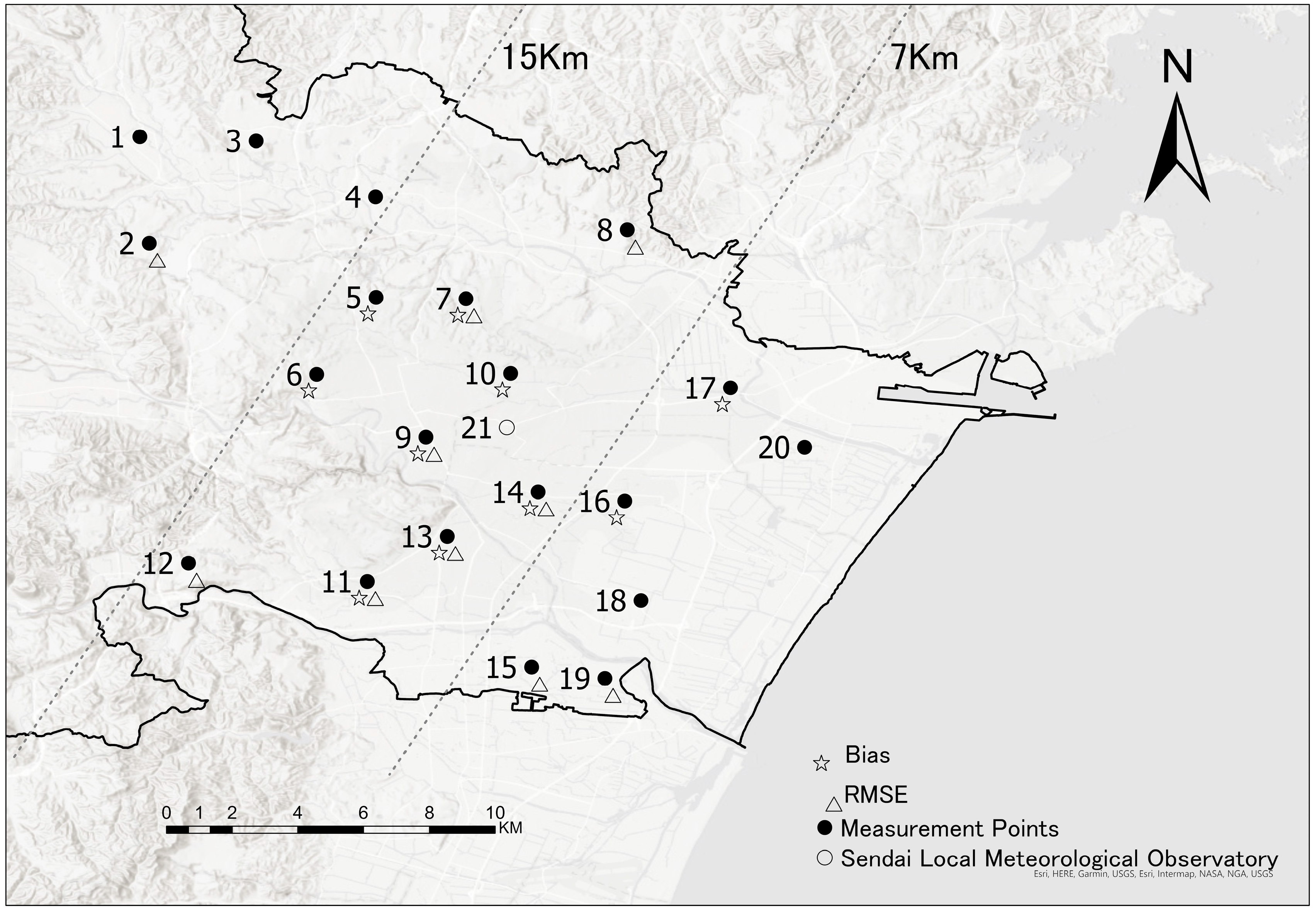
The Sendai Local Meteorological Observatory (38°15′43.60″ N, 140°53′49.52″ E) is located approximately 9 km inland within an urban zone. South of the observatory lies a park, while builtup areas occupy its northern and eastern sides. Meteorological instruments are deployed in an open area west of the main building. Continuous measurements include the air temperature, humidity, wind direction/speed, solar radiation, precipitation, and atmospheric pressure. All data—recorded at 10 min intervals—are accessible through the Japan Meteorological Agency. Wind speed data encompass both instantaneous and averaged values. An electronic hygrometer measures humidity, with temperature sensors mounted at 1.5 m above the ground level as per standard meteorological practice.

By downloading and sorting the data from the weather station, the climatic characteristics of Sendai were analyzed, and the target days that reflected most of the sea breeze days and west wind days were selected.

2.2.2. Long-Term Multi-Point Observation Data

This study defines temperature and humidity measurements from louver-mounted sensors as observational data. Long-term multipoint observation points were distributed in 20 elementary school playgrounds or parks in Sendai City. The main role of the data observed in this study was to verify the reproducibility of the simulated data.

In this study, according to the distance from the coastline and degree of urbanization, the study area was divided into three areas: inland (15–22 km from the coast), urban (7–15 km from the coast), and coastal areas (7 km from the coast). Twenty observation points (Table A1) were established across elementary schools and parks in Sendai City, with spatial distribution illustrated in Figure 2. The observation points extended inland from the coast, with four (1–4), ten (5–14), and six (15–20) observation points distributed in inland, urban, and coastal areas, respectively. To reduce observation interference and unify observation conditions, the observation sites were set on shallow grass away from buildings and trees. The recording frequency of the temperature and humidity sensors was set to 10 min.

Figure 2. Sendai city location, Sendai Local Meteorological Observatory, and temperature/humidity recorder placements, with symbols indicating the top 10 values of Bias (▲) and RMSE (★) from the WRF model reproducibility analysis. Detailed geographic information for each observation point is provided in Appendix A Table A1.

2.2.3. WRF Model Computes the Data

For this study, the mesoscale simulation was conducted using the Advanced Research WRF model, developed by the National Center for Atmospheric Research and the National Center for Environmental Prediction (NCEP), to model the Sendai urban area [72,73]. The simulated output was utilized to compute the “SBCC”. Key physical parameterizations for the model run are detailed in Table 1. The analysis primarily focused on Domain 3 simulation data, from which a uniformly spaced grid of 28 rows by 31 columns (spatial resolution: 1 km) was extracted. This 1 km resolution is standard for numerical investigations of urbanization and sea breeze phenomena [74,75]. Each grid point provided near-surface meteorological data, specifically the temperature and specific humidity at a 2 m height. The model output frequency was set at 10 min intervals to match the temporal resolution of the observational data.

Table 1. Computational parameterization of the WRF model.

Calculation period	09:00 (JST) on 1 August 2016 to 09:00 (JST) on 10 August 2016 (sea breeze day) 09:00 (JST) on 5 August 2013 to 09:00 (JST) on 15 August 2013 (west breeze day)
Vertical grid	30 layers (Ground Surface—50 hPa)
	Domain 1: 9 km, dimension 37 × 28
Horizontal grid (Figure 1b)	Domain 2: 3 km, dimension 43 × 34
	Domain 3: 1 km, dimension 31 × 28
Meteorological data	NCEP global reanalysis data
Land data	Digital national land information (resolution of 1000 m)
Microphysics	WSM 6-class graupel scheme
Radiation: Longwave	Rapid radiative transfer model
Shortwave	Dudhia shortwave scheme
PBL scheme	Mellor–Yamada–Janjic TKE scheme
Surface scheme	Urban canopy model

2.3. Determination of Study Day

2.3.1. Selection of Study Day

Based on meteorological station data obtained from the Japan Meteorological Agency (JMA), this study categorized target days into “sea breeze days” and “west wind days”. The difference in temperature between land and sea creates a difference in air pressure, which drives the air to move, thus forming wind. The screening was conducted based on the diurnal variation patterns of key meteorological variables. To minimize interference from extraneous factors, exclusively sunny days were selected as fundamental conditions during the preliminary target day screening process. The other specific conditions include the following:

Sunshine duration: at least 40% of potential sunshine hours.

Rainfall: no rainfall.

Cloud: <5% cloud.

Wind (sea breeze day): the wind blowing from the sea to the land lasts for at least 2 h.

Wind (west wind day): west wind for at least 2 h.

2.3.2. Study Day

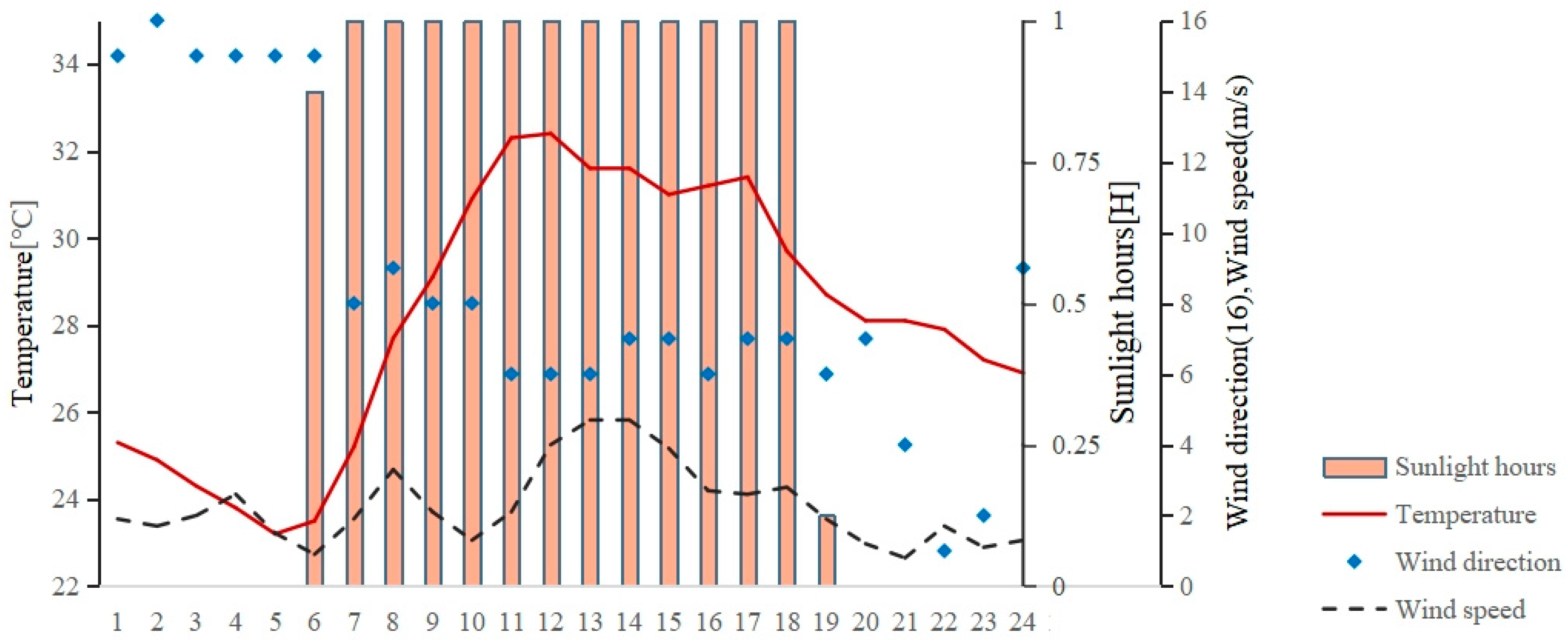
Building on prior analyses of Sendai’s sea breeze daily patterns, this study selected the three-year period from summer 2018 to 2020. This period closely matched the 12-year average daily temperature curve for sea breezes (summers 2010–2021). Given that sea breezes arrive between 11:00 and 12:00 on over 60% of days when the maximum temperatures exceed 30 °C [76], we focused specifically on sea breeze days with arrival times at these two hours. To meet the required meteorological conditions, only days with a stable wind direction after the sea breeze made landfall were included. Finally, 5 August 2016 (Figure 3) was selected as the study day of a “sea breeze day” in this study.

Figure 3. Meteorological parameters for 5 August 2016 encompassed sunlight duration, temperature, wind direction, and wind speed. Note: the wind direction scale of 1–16 denotes the 16 compass directions, where 1: N, 2: NNE, 3: NE, …, 16: NNW.

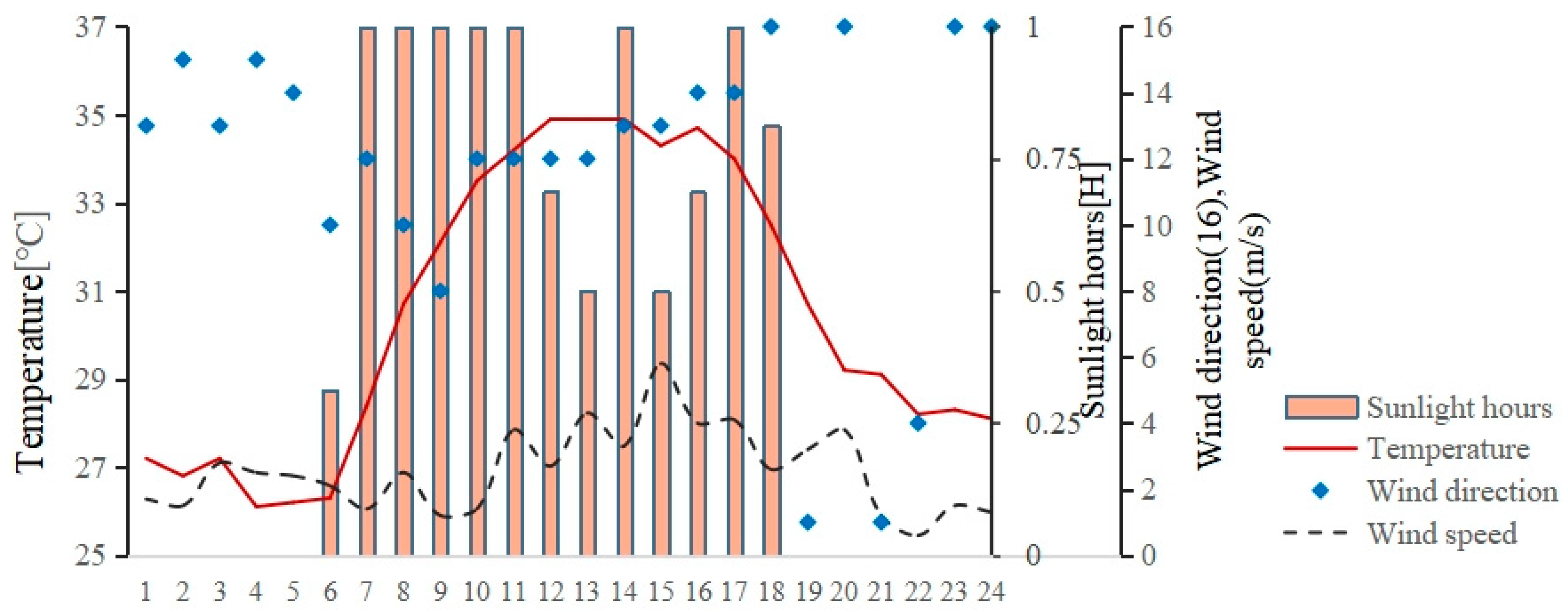
This is because the frequency of westerly days was much lower than that of sea breeze days. In theory, the airflow always moves from high pressure to low pressure; therefore, the wind always blows from the cooler side to the warmer side. Therefore, on sunny and hot days, the sea breeze will blow. Finally, 10 August 2013 was selected as the case study day based on the meteorological observations downloaded by the Japan Meteorological Agency. On the case study day, there was no rain all day, the maximum temperature was 34.9 °C, and the wind blew from the land to the sea from 10:00 to 17:00 (Figure 4).

Figure 4. Meteorological parameters for 10 August 2013 encompassed sunlight duration, temperature, wind direction, and wind speed. Note: the wind direction scale of 1–16 denotes the 16 compass directions, where 1: N, 2: NNE, 3: NE, …, 16: NNW.

3. Reproducibility Analysis of WRF Model Simulation Results

Compared with microclimate research, in urban climate research, owing to the large scale of cities, a small number of observation points, and uneven distribution, the data in the research cannot meet the research on the urban climate. To compensate for this defect, an increasing number of researchers have begun to use the WRF model to reproduce the urban climate. For example, Takebayashi used the WRF model to analyze the relationship between the urban size, land use, temperature rise, and coastal distance in coastal cities in Japan and Germany in summer [77]. Sasaki used the WRF model to build an urban environmental climate map that shows the distribution patterns of wind and temperature in a city [78]. Utilizing the WRF model, Peng simulated the spatial extent of sea breeze cooling and specific humidity enhancement [71]. This model is primarily designed for large-scale numerical weather prediction. Therefore, compared to smaller mesoscale urban climate studies, there are certain differences between the simulation results and real values. The data output by the WRF model is temporal and spatial, and this study verified the repeatability of the simulated and measured values in terms of the time series and spatial location, which supports the exploitability of all data in later calculations.

3.1. Analysis of Bias, Root Mean Squared Error (RMSE), and Correlation

The reproducibility of the WRF model data was evaluated by pairing simulated outputs with actual measurements at corresponding points for comparative analysis. The simulation points were uniformly distributed in the simulation domain, whereas the measurement points were randomly distributed in the playgrounds of each elementary school in Sendai. Therefore, there was a certain deviation in the positions of the simulated and measured points, and they did not coincide completely. Since the simulated points uniformly covered the entire study area, there was always a point closest to the measured point. Each monitoring station was matched to its nearest model grid point for data comparison. Table 2 lists the specific locations and distances between the measured and simulated points.

Table 2. The locations of the measured and simulated points and the distance between them.

ID	Station Name	Lon.	Lat.	FID	Lon.	Lat.	Distance (km)
1	Nenoshiroishi	140.7966	38.3417	731	140.7933	38.3416	0.29
2	Yakata	140.7992	38.3126	633	140.8047	38.3144	0.54
3	Teraoka	140.8284	38.3406	734	140.8279	38.3416	0.12
4	Nomura	140.8611	38.3253	671	140.8627	38.3235	0.24
5	Kita-Sendai	140.8612	38.2978	572	140.8627	38.2963	0.21
6	Kunimi	140.8450	38.2767	504	140.8395	38.2781	0.51
7	Asahigaoka	140.8857	38.2974	574	140.8858	38.2963	0.12
8	Tsurugaoka	140.9299	38.3162	644	140.9320	38.3144	0.27
9	Higashi Nibancho	140.8748	38.2595	441	140.8742	38.2600	0.08
10	Saiwaicho	140.8979	38.2770	509	140.8973	38.2781	0.14
11	Nishitaga	140.8588	38.2199	308	140.8627	38.2237	0.54
12	Hitokita	140.8099	38.2249	303	140.8049	38.2237	0.46
13	Nagamachi	140.8806	38.2323	343	140.8858	38.2328	0.46
14	Minamikoizumi	140.9054	38.2444	378	140.9089	38.2419	0.41
15	Fukurobara	140.9037	38.1965	213	140.9089	38.1965	0.45
16	Kabanomachi	140.9292	38.2419	380	140.9320	38.2419	0.25
17	Takasago	140.9581	38.730	481	140.9551	38.2691	0.51
18	Rokugo	140.9336	38.2147	281	140.9319	38.2146	0.15
19	Higashishiromaru	140.9238	38.1934	214	140.9204	38.1965	0.45
20	Okada	140.9784	38.2567	450	140.9782	38.2600	0.37

This study evaluated the reproducibility between measured and simulated datasets by examining the Bias, RMSE, correlation coefficients, and error metrics. Bias is used to indicate the degree of fit between the simulated and true values. A smaller absolute value indicates a higher degree of fit and vice versa. The average value of all simulated points covered within the range of the measured point is defined as S (Simulated) and the measured value of each measured point is Mn (Measured); therefore, the calculation formula of the deviation is Bias = S-MN. RMSE is a measure of precision that is often used to measure the difference between the predicted or estimated value of a model and the observed value. The formula used is as follows:

$$RMSE=\sqrt{{\displaystyle \frac{{\sum }_{i=1}^n{\left(X_{mea,i-}{X}_{sim,i}\right)}^2}{n}}}$$

Correlation analysis was used to analyze the degree of correlation between the pairs of variables. In this study, the RMSE and correlation were calculated using SPSS software(version 26.0).

Table 3 lists the Bias, RMSE, and correlation calculation results. According to the data analysis, the correlation of all points is strong. After sorting the difference values of Bias and RMSE from large to small, the top 10 with large differences are marked in Figure 2. Among them, the difference values of Bias and RMSE are larger at the same time in points 7, 9, 11, 13, and 14. Figure 2 shows that all five points are distributed in urban areas. The difference increases with higher urbanization. This is the same conclusion reached in previous studies.

Table 3. Precision assessment results of temperature numerical computation. The spatial distribution of these assessment results is shown in Figure 2.

ID	Location	RMSE [°C]	Bias [°C]	Correlation
1	Nenoshiroishi	0.68	−0.55	0.981
2	Yakata	0.82	−0.88	0.973
3	Teraoka	0.82	−0.76	0.974
4	Nomura	0.43	−0.13	0.993
5	Kita-Sendai	0.57	−1.36	0.984
6	Kunimi	0.53	−1.81	0.985
7	Asahigaoka	0.99	−1.72	0.945
8	Tsurugaoka	1.09	−0.62	0.945
9	Higashi Nibancho	1.00	−2.49	0.936
10	Saiwaicho	0.58	−1.53	0.979
11	Nishitaga	0.99	−2.05	0.939
12	Hitokita	0.88	−0.24	0.969
13	Nagamachi	0.86	−2.13	0.950
14	Minamikoizumi	0.88	−2.15	0.937
15	Fukurobara	1.03	−0.84	0.912
16	Kabanomachi	0.53	−1.29	0.969
17	Takasago	0.80	−1.36	0.957
18	Rokugo	0.82	−1.20	0.926
19	Higashishiromaru	1.34	−0.60	0.802
20	Okada	0.75	−0.59	0.939

3.2. Error Dynamics Analysis

According to Section 3.1, the difference between the observed and simulated data was regional, whereas that of the meteorological data was temporal. Therefore, an error analysis of the observed and simulated data for 24 h a day was conducted from different partitions (inland, urban, and coastal areas) to further analyze the difference between the observed and simulated data. The error is defined as follows: Let the Nth measured value at measurement point A be A_n and select the simulation point B that is closest to measurement point A in spatial location, with its Nth simulated value denoted as B_n. The deviation between the simulated and measured results is then quantified by calculating the difference between the Nth values of these two points, i.e., the deviation value X_n = B_n − A_n. In other words, Xn = Bn − An. The average temperature at each time point was used for the error calculation, which was calculated separately for the entire area and the three partitions.

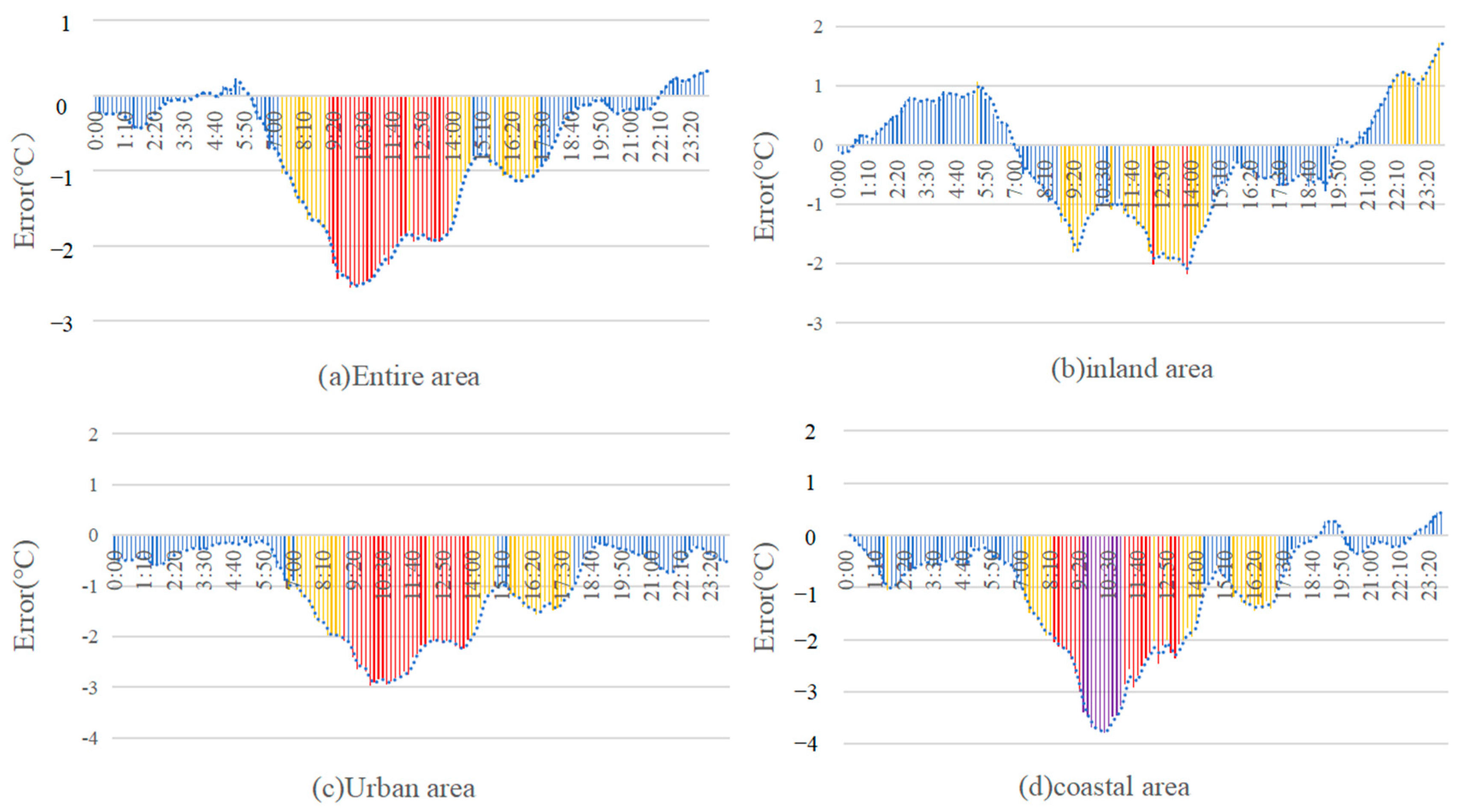
By analyzing the error dynamic graph of the entire area error (Figure 5), it can be observed that the error value is always negative in the daytime period (06:00–19:00), which means that the simulated value is always lower than the observed value in the daytime.

Figure 5. Error dynamic curves for the (a) entire, (b) inland, (c) urban, (d) and coastal areas.

According to the analysis of the regional error dynamic graph (Figure 5), the error value is always negative in the daytime (06:00–19:00) in the entire area, which means that the simulated value is always lower than the observed value in the daytime. The time interval where the error exceeds 2–3 °C is 9:20 to 11:50, where the peak occurs at 10:00 am. Compared with the entire area, the error value in the inland area increased in the night-time (20:00–07:00), that in the daytime (07:00–20:00) between 0 °C and 1 °C was significantly increased, and the maximum error value (−2 °C) was also reduced. However, in urban areas, errors remain negative all day, indicating that simulated temperatures are consistently lower than observed. During the morning (09:00–13:30), these errors peak, ranging from 2–3 °C. The error value is small (0–1 °C) in the night-time (19:00–06:00). In coastal areas, the night-time (19:00–06:00) still shows a small error value (0–1 °C), whereas the daytime, particularly 09:30–11:00, has a large error value between 3 °C and 4 °C.

From the above analysis, it can be concluded that there is a strong correlation between the simulated and measured values at each point. Among the three regions, the difference was highest in urban areas. In the dynamic error analysis, simulated values consistently fell below measured values across most regions and times, with the exception of certain local periods in inland areas. The time window of 10:00–12:00 consistently exhibits the highest errors during daylight hours. Among the three regions analyzed, the coastal region exhibited locally elevated errors, while the inland region demonstrated the lowest error levels.

4. Calculation of SBCC

This study employed the WRF model to simulate urban temperatures in Sendai, Japan, under sea breeze and westerly wind conditions. The computed temperature difference between these scenarios quantifies the sea breeze’s cooling capacity for coastal cities. This differential represents the reduction in urban temperature attributable to the sea breeze influence under comparable weather conditions. This difference was defined in this study as the cooling ability of sea breezes in coastal cities.

The choice of sea breeze and west wind days was made by considering days with similar weather conditions. However, temperature is affected by current weather conditions and by climate phenomena that have already occurred in the previous period.

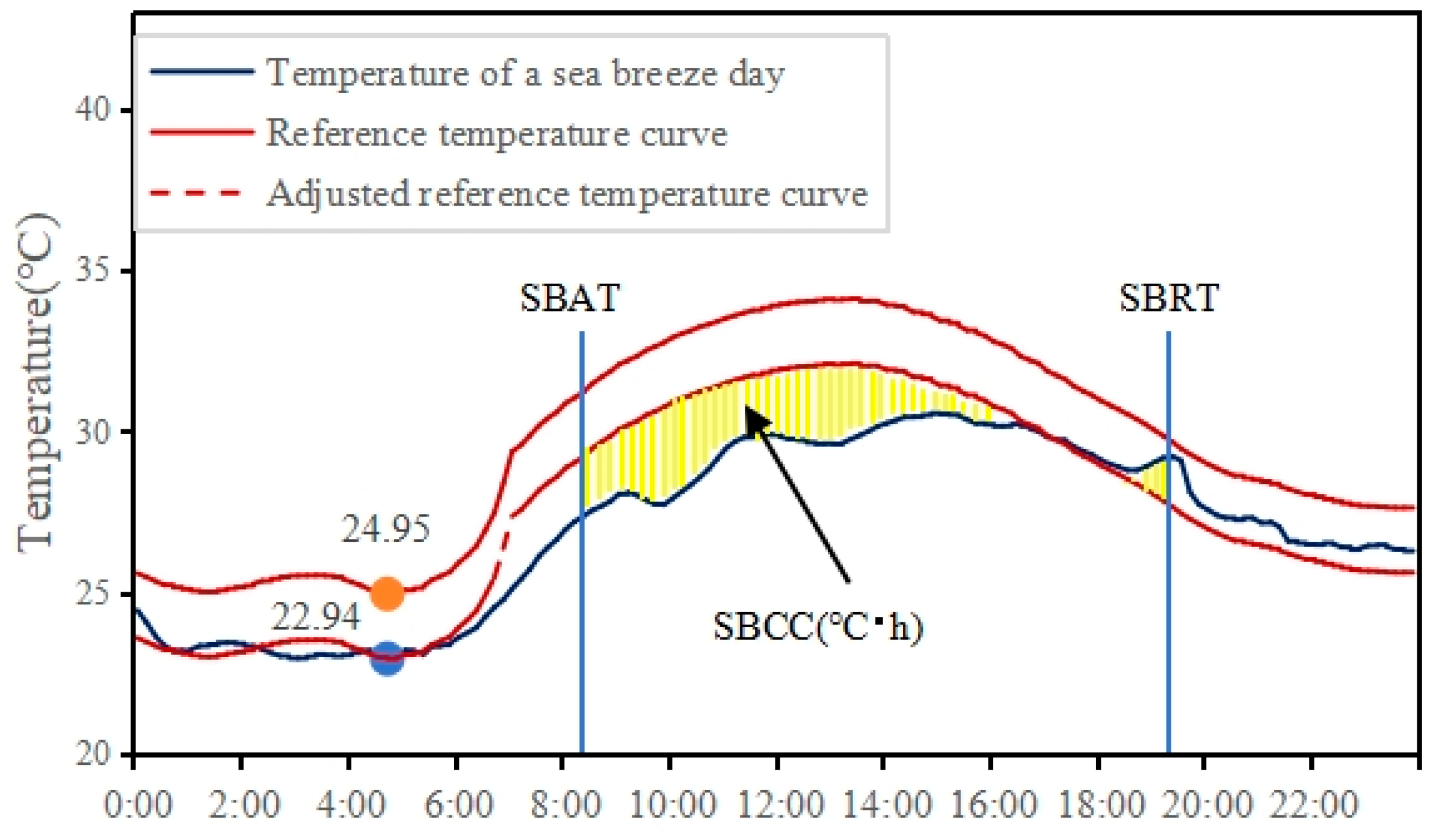
A comparison of the simulated temperature curves revealed that temperatures were lower on the sea breeze day even during the early morning hours prior to sunrise. As sea breezes are a daytime phenomenon, this nocturnal cooling was likely attributable to other meteorological factors, such as enhanced radiative cooling or land breeze effects. To ensure that the calculated Sea Breeze Cooling Capacity (SBCC) solely reflects the cooling effect of the sea breeze itself, we applied a baseline adjustment to the westerly wind day’s temperature profile, excluding non-sea-breeze-related temperature differences.

Therefore, all temperature values on westerly days must be adjusted. The specific method of adjustment was to extract the lowest temperature value in the morning of the west wind day (orange point in Figure 6) and then find the temperature value of the sea breeze day at the same time (blue point in Figure 6). The temperature difference between these two values represents a uniform offset that was subtracted from all temperature values on the westerly wind day to establish a comparable baseline before the sea breeze influence. After the temperature of the west wind day was adjusted, the SBCC was calculated.

Figure 6. Study area temperature profiles at Sendai simulation point: sea breeze conditions (5 August 2016), westerly wind conditions (10 August 2013), and corresponding modified profiles. Yellow denotes SBCC (Sea Breeze Cooling Capacity). SBAT indicates sea breeze arrival time, SBRT signifies sea breeze retreat time. Note: the inflection point around 7:00 in the westerly wind day curve reflects changes in the warming rate due to boundary layer development under clear-sky conditions.

The SBCC is defined as the difference between the time-integrated temperature under westerly wind conditions (WESTA) and that under sea breeze conditions (SEA). The SBCC (°C.h) is defined as the product of sea breeze cooling and the cooling time (shaded area in Figure 6). The calculation method is shown in Equation (1), where WESTA and SEA are the time integrals of the adjusted westerly and sea breeze daily temperature curves, respectively. These were defined using Equations (2) and (3), respectively:

SBCC = WESTA – SEA

(1)

$$WESTA=\sum _{i=2}^n{\displaystyle \frac{\left(T_{west\left(i-1\right)}+T_{west\left(i\right)}\right)\times ∆t}{2}}$$

(2)

$$SEA=\sum _{i=2}^n{\displaystyle \frac{\left(T_{sea\left(i-1\right)}+T_{sea\left(i\right)}\right)\times ∆t}{2}}$$

(3)

where T_west(i) and T_sea(i) denote temperatures from the adjusted westerly wind curve and sea breeze curve at timestep I, respectively, Δt represents the timestep interval during sea breeze events, and n is the total timestep count. The timestep count per location defines the local sea breeze duration, calculated from arrival to retreat times. The timing data referenced a sea breeze action chart [78].

It is important to note that the SBCC metric is calculated solely from the near-surface air temperature at a 2 m height, reflecting the cooling capacity within the atmospheric layer most associated with human activity. While the vertical structure and depth of the sea breeze undoubtedly influence its surface manifestation, a detailed analysis of these factors is beyond the scope of this study.

5. Results and Discussion

5.1. SBCC

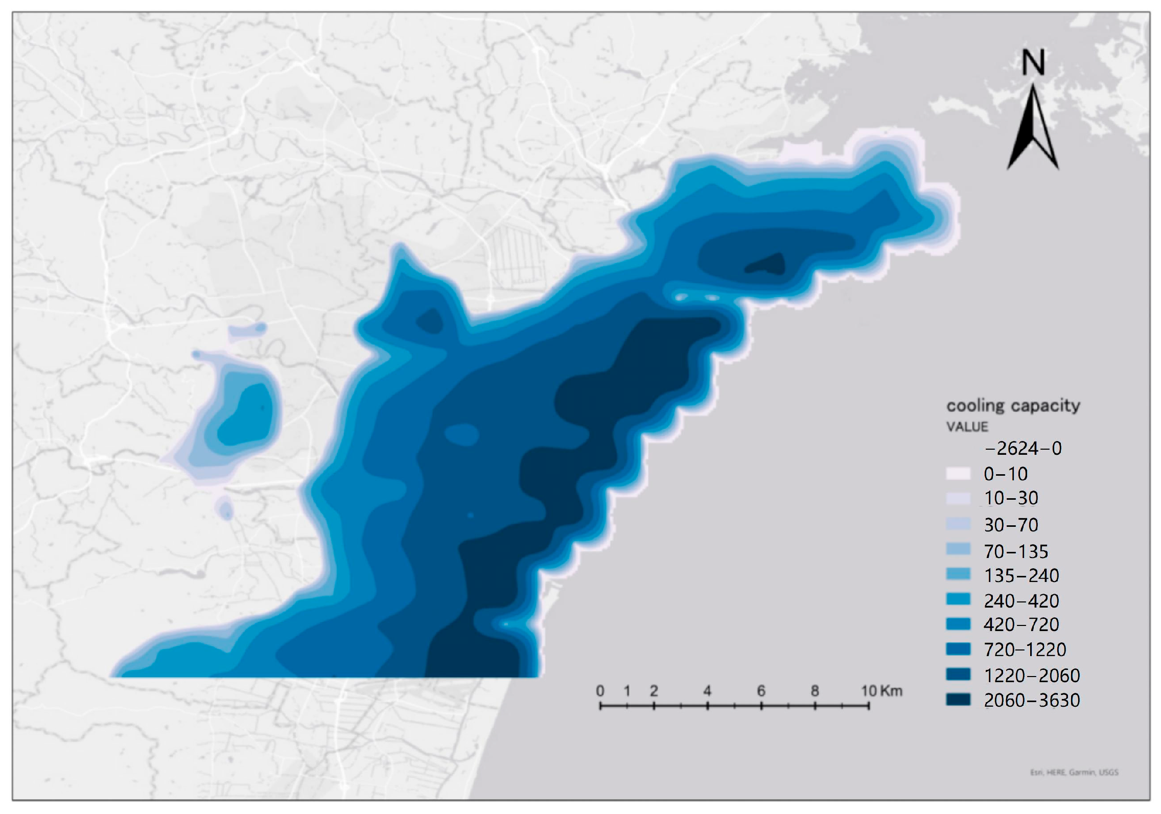
After simulation by the WRF model according to the selected sea breeze day and west wind day, data for 1089 points were obtained. The geographic coordinate and temperature data for each point were exported. Consequently, the Sea Breeze Cooling Capacity (SBCC) was determined for each location. These values were subsequently visualized using ArcGIS Pro to generate a spatial distribution map of the SBCC across the study area (Figure 7).

Figure 7. Spatial distribution of cooling induced by sea breezes throughout their active period.

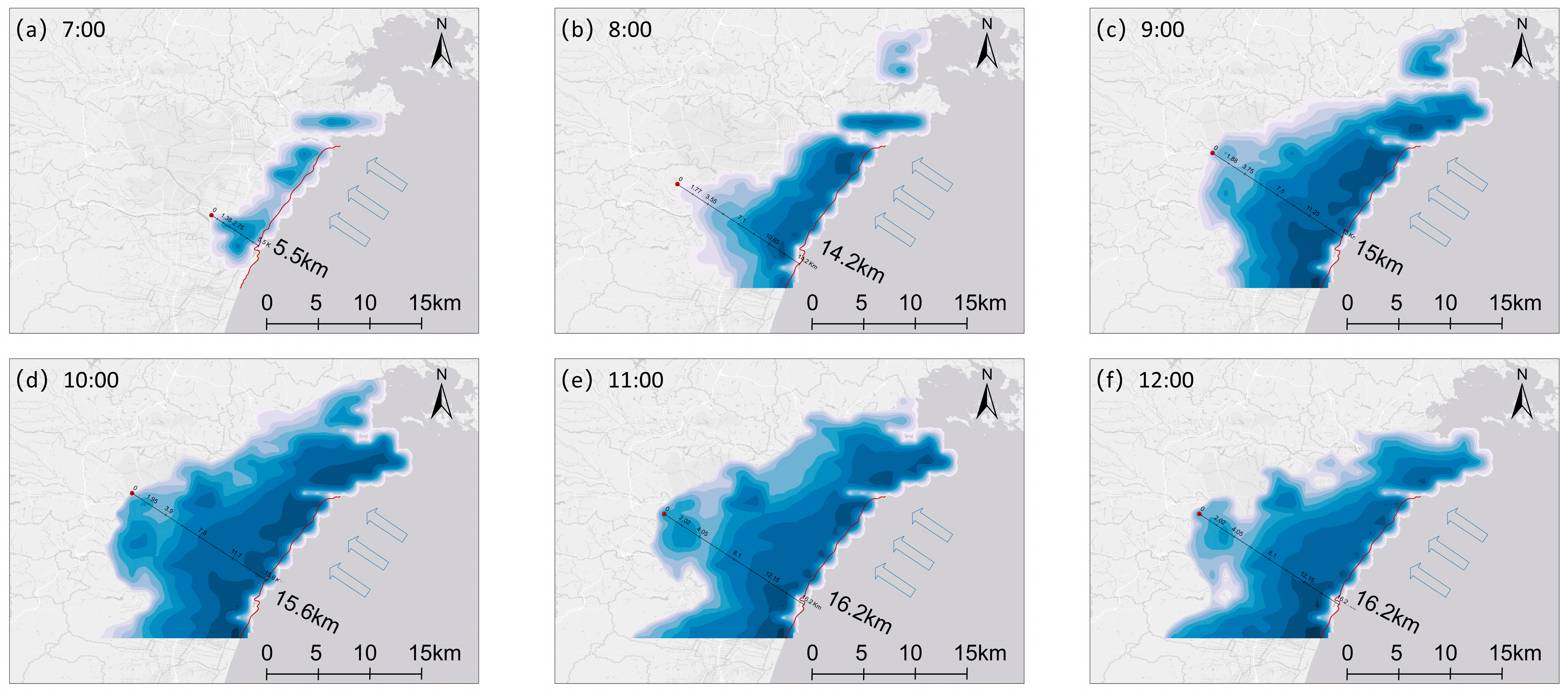
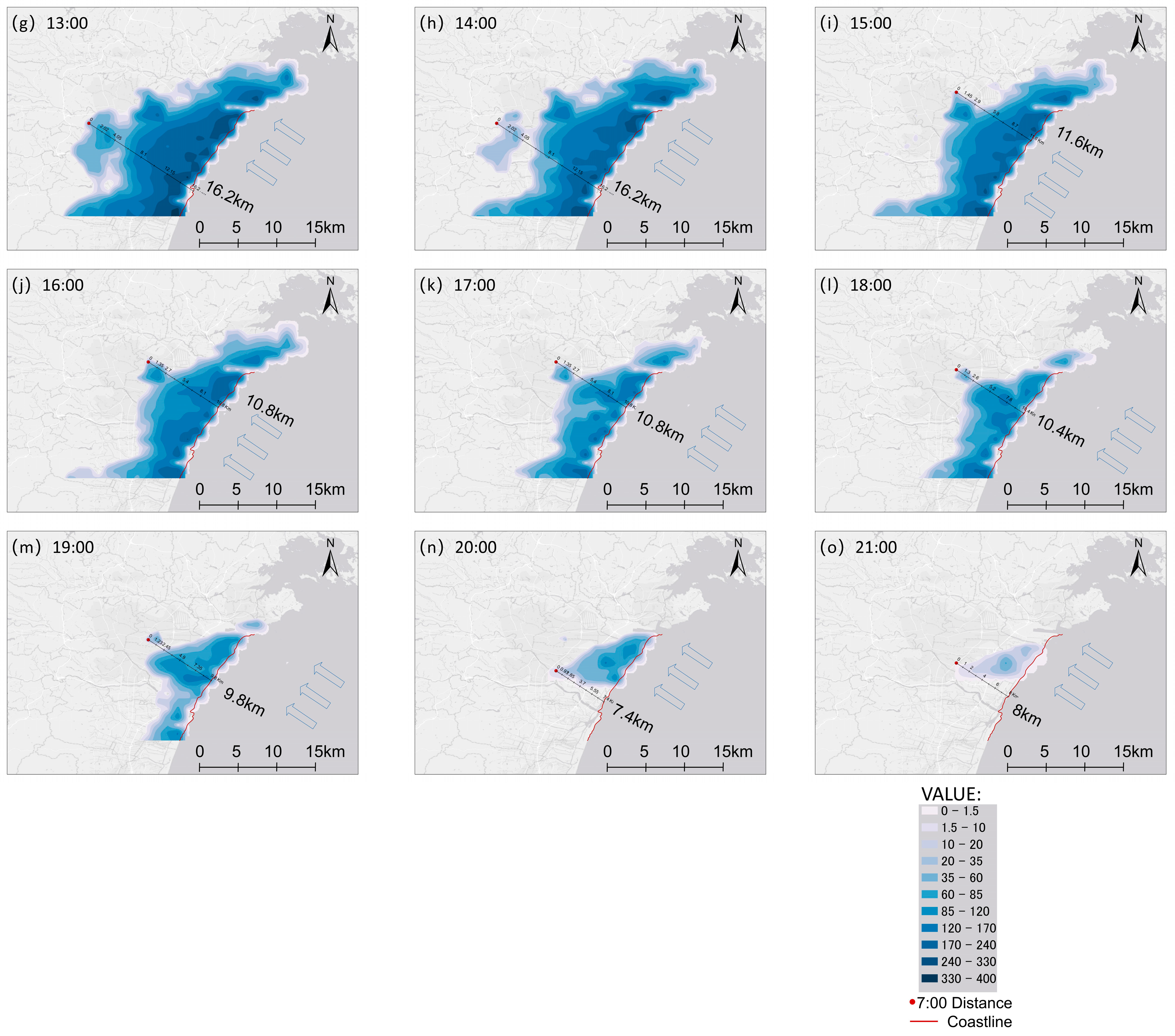
As shown in Figure 7, the blue area represents a positive value of the SBCC, that is, the SBCC is generated at this point, and different shades of color represent different cooling intensities. Through observations, it was found that the SBCC has certain characteristics. The sea breeze cooling intensity is most pronounced along the coast and attenuates progressively with the distance inland.

5.2. Trend of SBCC and Cooling Range over Time

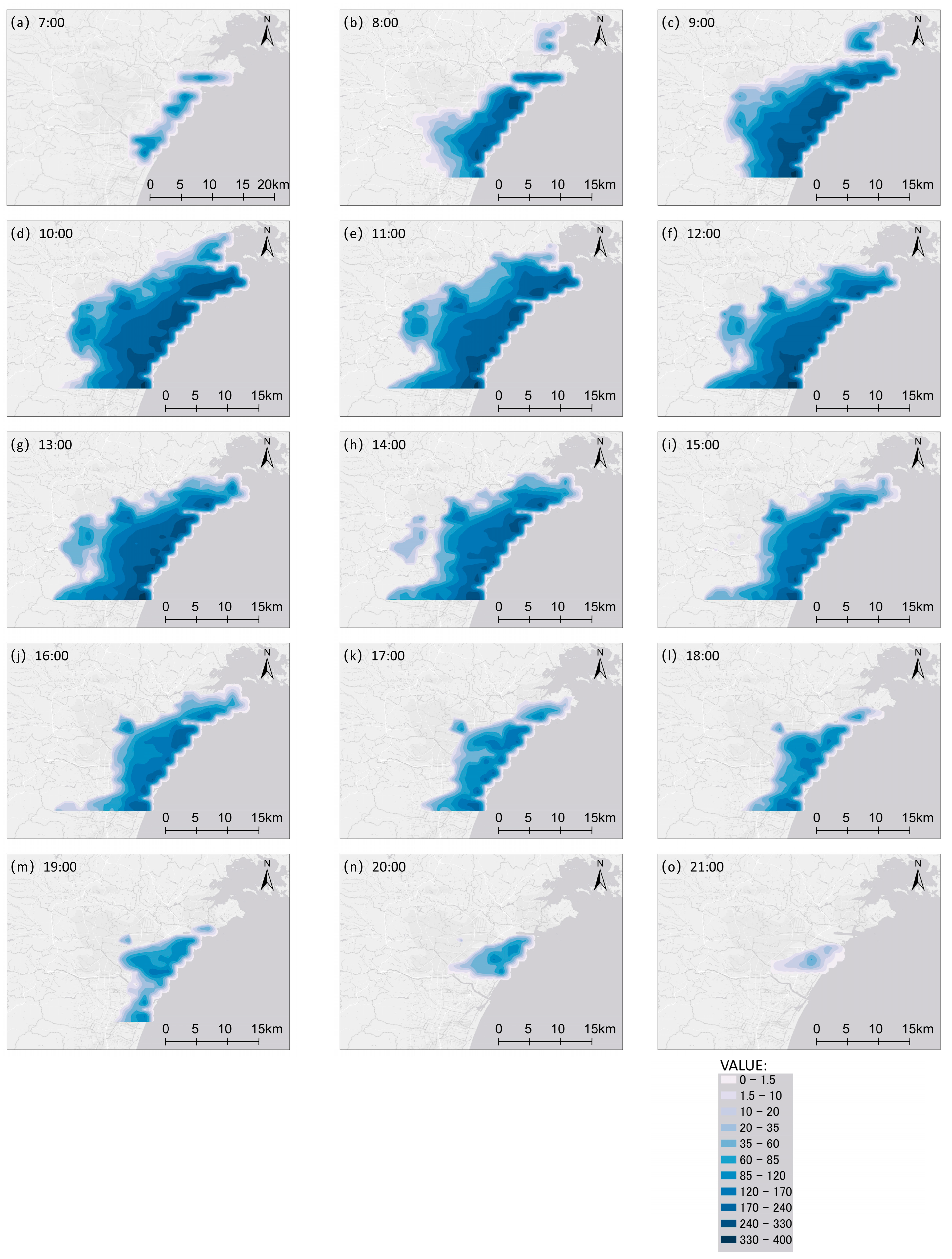
Under sea breeze conditions, the SBCC characteristics at each point were determined through hourly analysis. The calculation time interval was the SBCC for 15 h from 07:00 to 21:00 (determined according to the sea breeze action time interval in the study area).

After visualizing the data using ArcGIS Pro, the changes in the SBCC and cooling range could be visualized intuitively. The change process starts with a small intensity and range at 07:00, gradually increases and diffuses, and then gradually decreases and shrinks (Figure 8). Moreover, the sea breeze cooling range is geographically distributed in different time periods in the study area.

Figure 8. Plan view of SBCC per hour.

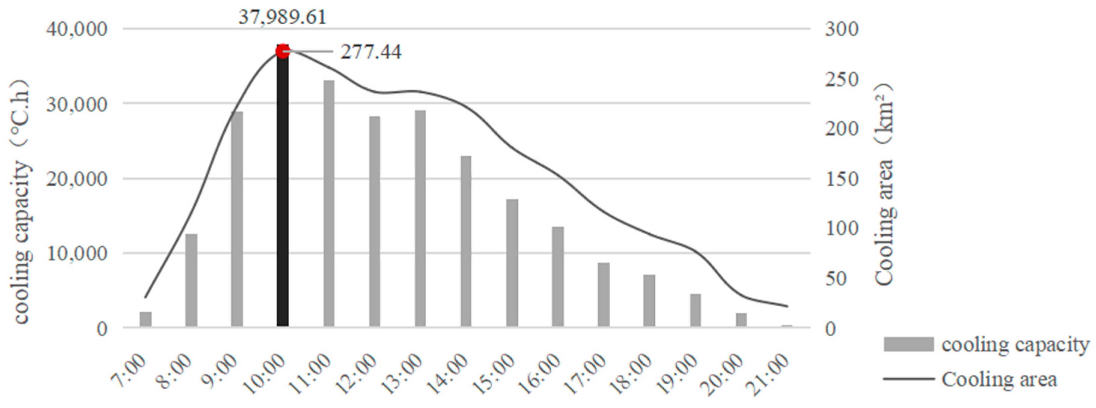
A statistical analysis of the data (Figure 9 and Table A2) revealed that the cooling capacity and range of the sea breeze showed an initial increase followed by a decrease. At 10:00, the SBCC peaked at 37,989.61 °C.h, while the cooling range reached its maximum extent of 277.44 km². From 07:00 to 10:00, there was a rapid increase; in 3 h, the cooling capacity and range increased from 2092.995 °C.h to 37989.61 °C.h and 30.6 km² to 277.44 km², respectively, increasing by 18 and 9 times, respectively.

Figure 9. SBCC and cooling area per hour. Detailed data are provided in Appendix A Table A2.

After 10:00, the cooling capacity and range began to decline; between 10:00 and 13:00, the decline rate was slower; and from 12:00 to 13:00, there was a small increase. After 13:00, the cooling capacity and cooling range exhibited a continuously declining trend and the rate of decline was more uniform.

5.3. SBCC and Distance

This section examines the relationship between the SBCC and distance. Here, distance is defined as the measurement along the sea breeze direction from the coastline to the location where its cooling effect is observed. The associations of both the cumulative and hourly SBCC with distance under all observed sea breeze cooling events were analyzed.

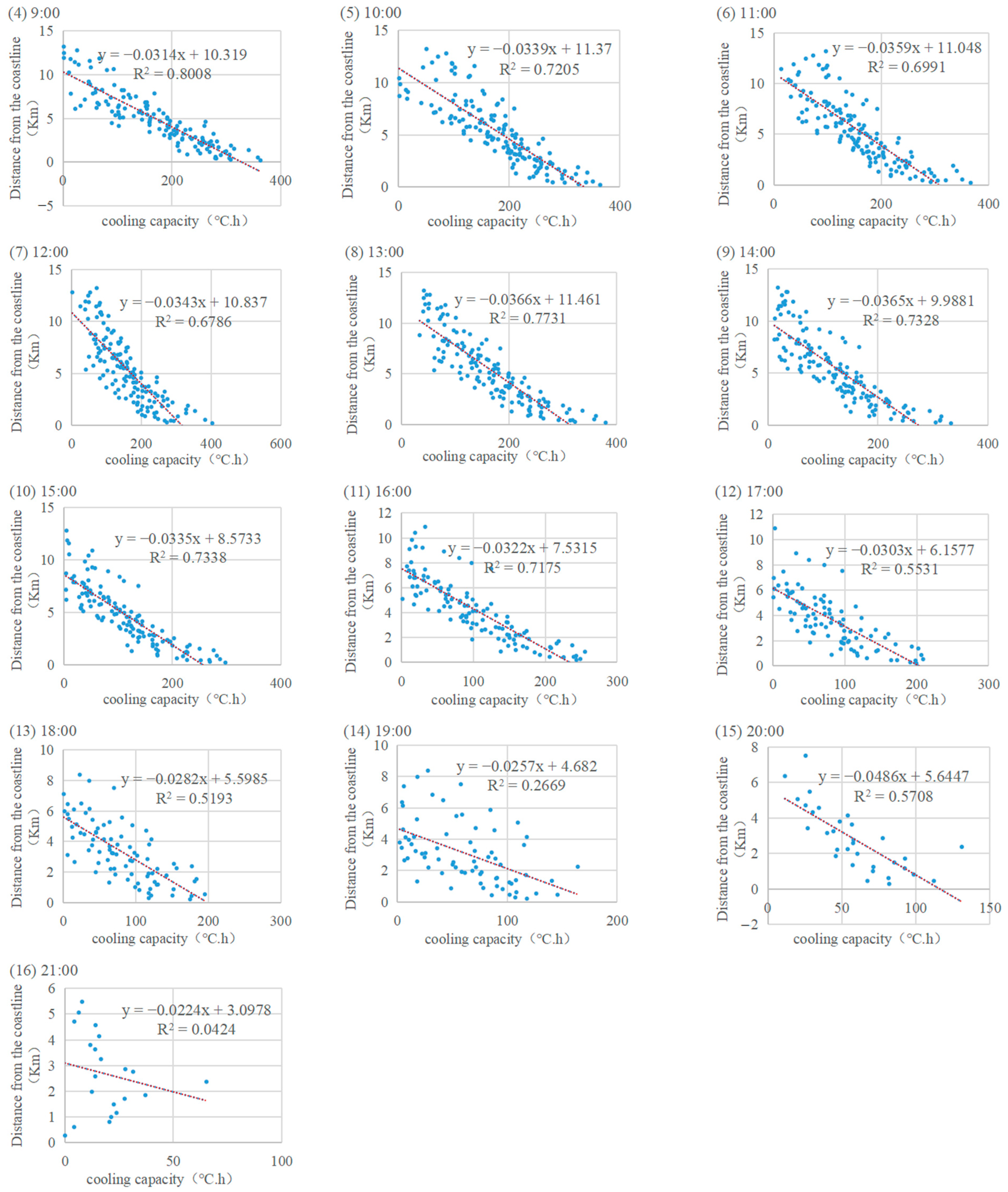
Figure 10 shows the scatter plot and trend line of the total cooling capacity and hourly cooling capacity of the sea breeze versus distance for all sea breeze cooling actions. The formula and value of R squared are attached. All relationships except for 07:00 were positive and had a low fit (R² = 0.0083). The remaining time showed a negative correlation with a good fit from 08:00 to 16:00. The sea breeze cooling capacity (SBCC) exhibits a strong negative correlation with distance from the coast, indicating significantly enhanced cooling effects in areas closer to the shoreline.

Figure 10. SBCC as a function of distance.

Table 4 summarizes the correlation coefficients between the SBCC and distance at all times. The absolute values of the correlation coefficients at 07:00, 19:00, and 21:00 were <0.7. All the remaining times had a strong negative correlation.

Table 4. The correlation between cooling capacity and distance. Time zone is JST.

ALL	−0.724
7:00	0.091
8:00	−0.817
9:00	−0.895
10:00	−0.849
11:00	−0.836
12:00	−0.824
13:00	−0.879
14:00	−0.856
15:00	−0.857
16:00	−0.847
17:00	−0.744
18:00	−0.721
19:00	−0.517
20:00	−0.756
21:00	−0.206

5.4. Inland Penetration Distance of Sea Breeze Cooling

To quantify the inland advancement of sea breeze cooling, hourly measurements determined the maximum penetration distance from the coastline (Figure 11). This distance, representing the farthest extent of the cooling influence, was individually assessed according to the sea breeze cooling spatial distribution maps and coastal wind direction.

Figure 11. Hourly maximum penetration distance of the sea breeze cooling area.

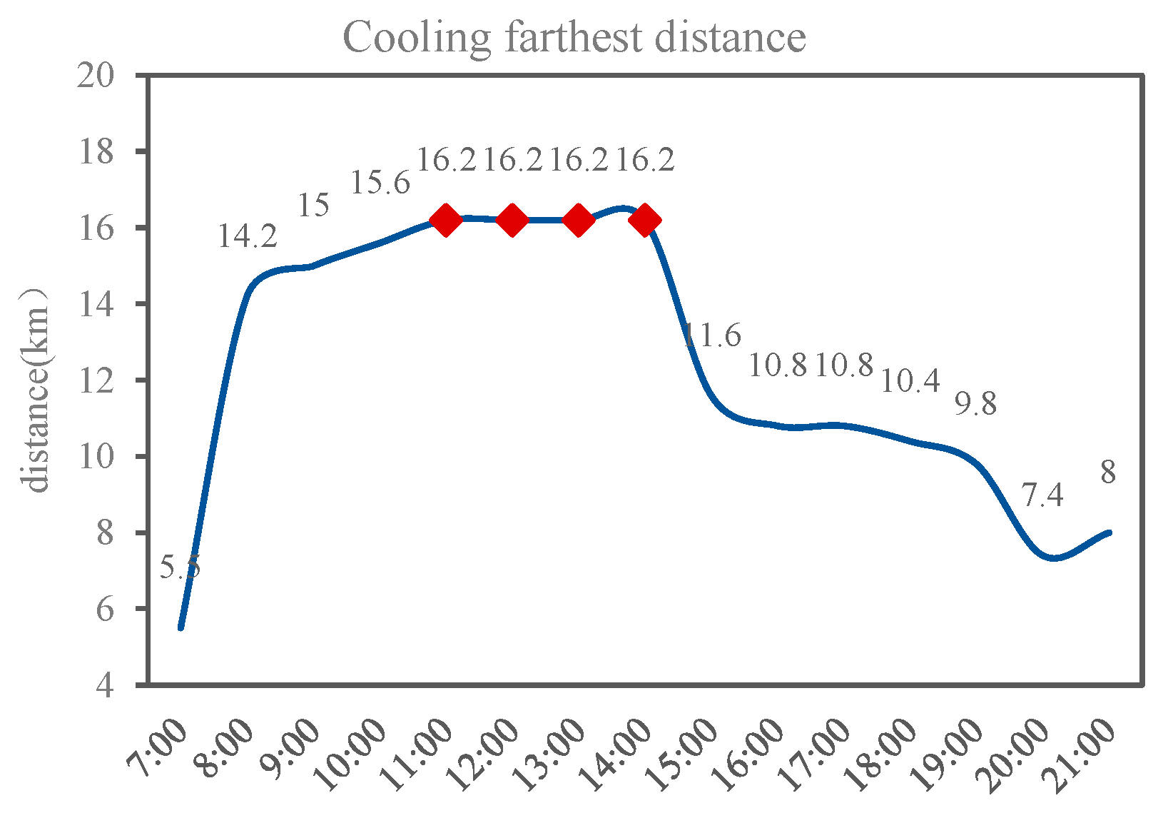
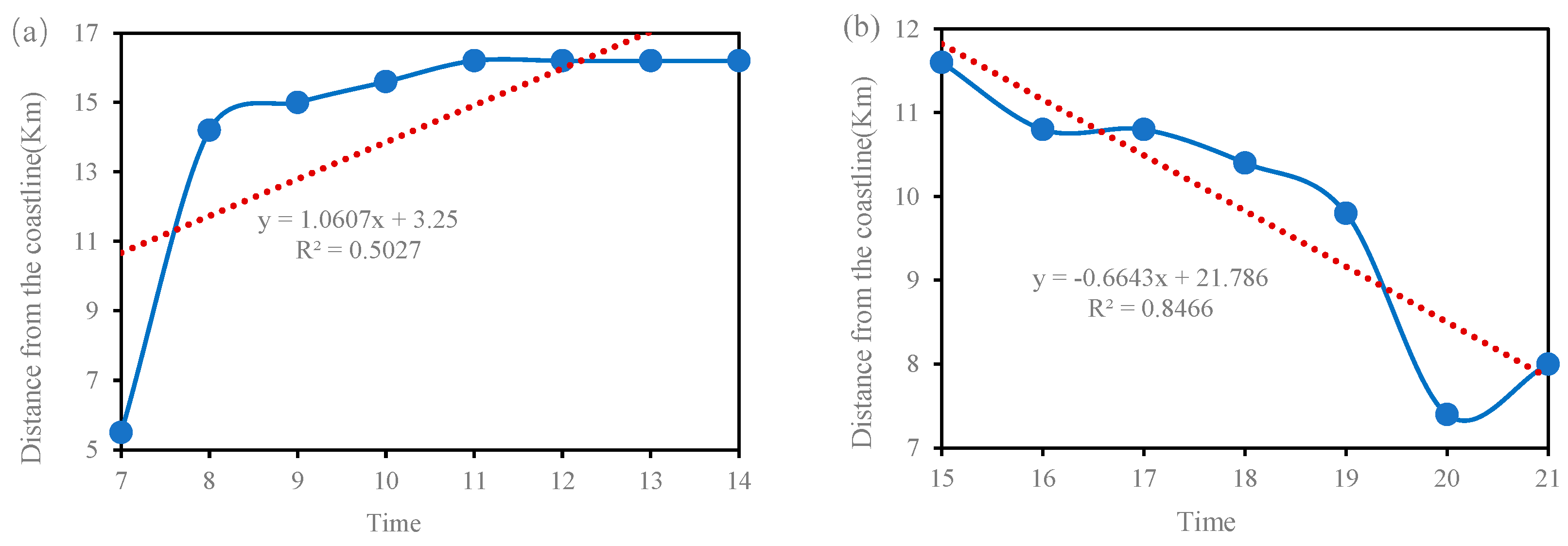
At 07:00, the longest distance was 5.5 km; the 08:00 distance rapidly increased to 14.2 km; at 11:00, the cooling distance reached 16.2 km; and after 14:00, it quickly decreased. Subsequently, a downward trend is observed (Figure 12). In terms of the relationship between the cooling distance and time (Figure 13), there was a positive correlation from 07:00 to 14:00, and the correlation coefficient was 0.71 after calculation. There was an obvious negative correlation from 15:00 to 21:00 and the correlation coefficient was −0.92.

Figure 12. Farthest cooling distance and time.

Figure 13. (a) The 7:00–14:00 farthest cooling distance and time; (b) 15:00–21:00 farthest cooling distance and time.

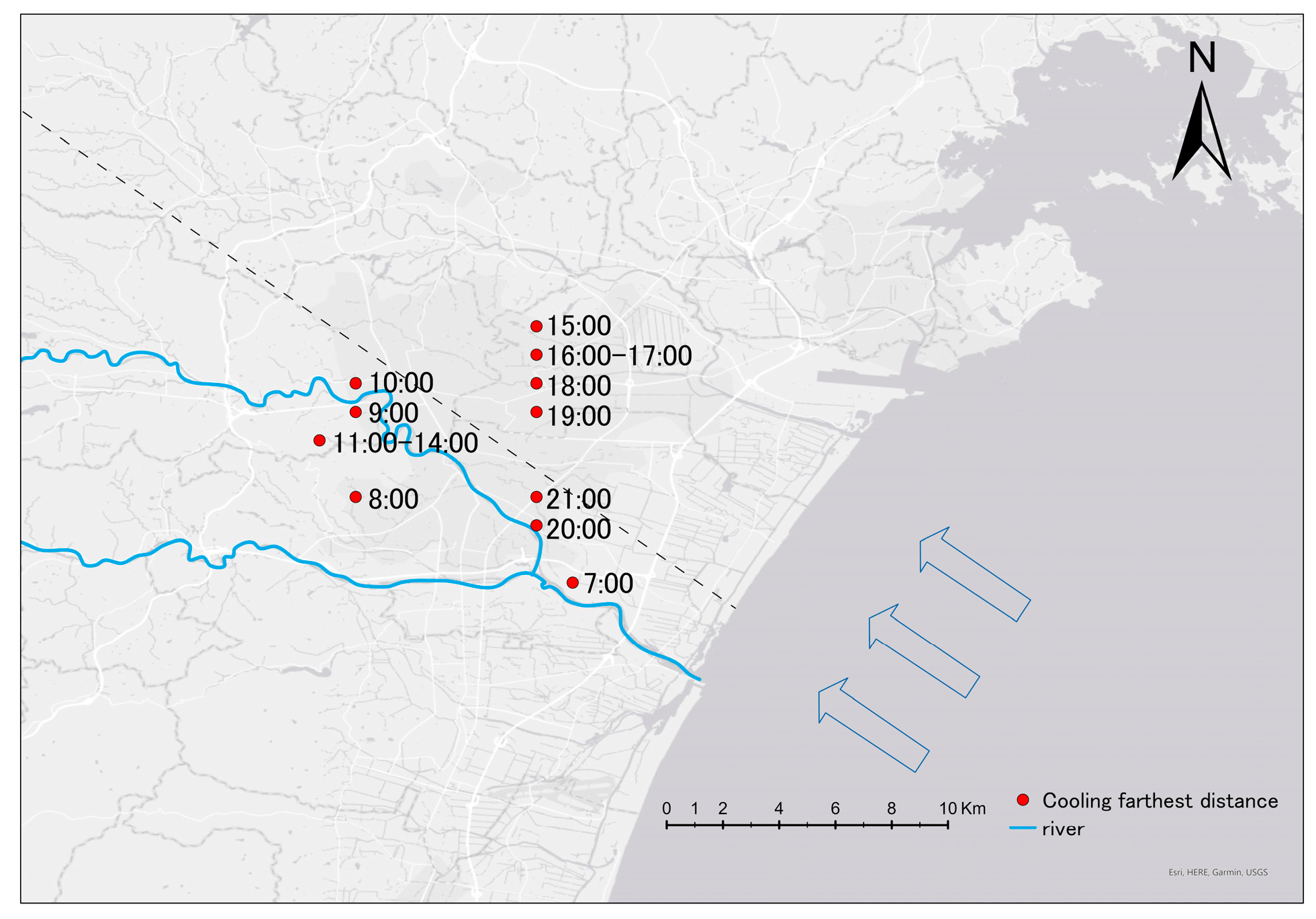
The point with the farthest sea breeze cooling distance from 7:00 to 21:00 is represented on the map (Figure 14). An analysis of the distribution map intuitively indicates that the penetration of cooling aligns with the sea breeze direction. During the periods 7:00–14:00 and 20:00–21:00, ten monitoring points were clustered near the inland river, while between 15:00 and 19:00, five points were located relatively farther from the river. Points exhibiting the greatest sea breeze cooling distance demonstrated an enhanced cooling capacity and a broader cooling extent along the sea breeze path. Further analysis is required for the point where the inland river is most distant from the sea breeze cooling capacity (SBCC).

Figure 14. Hourly farthest cooling point on the map. The arrow direction indicates the ‘sea breeze’ direction defined in this study, which represents the prevailing wind direction during summer in the research area.

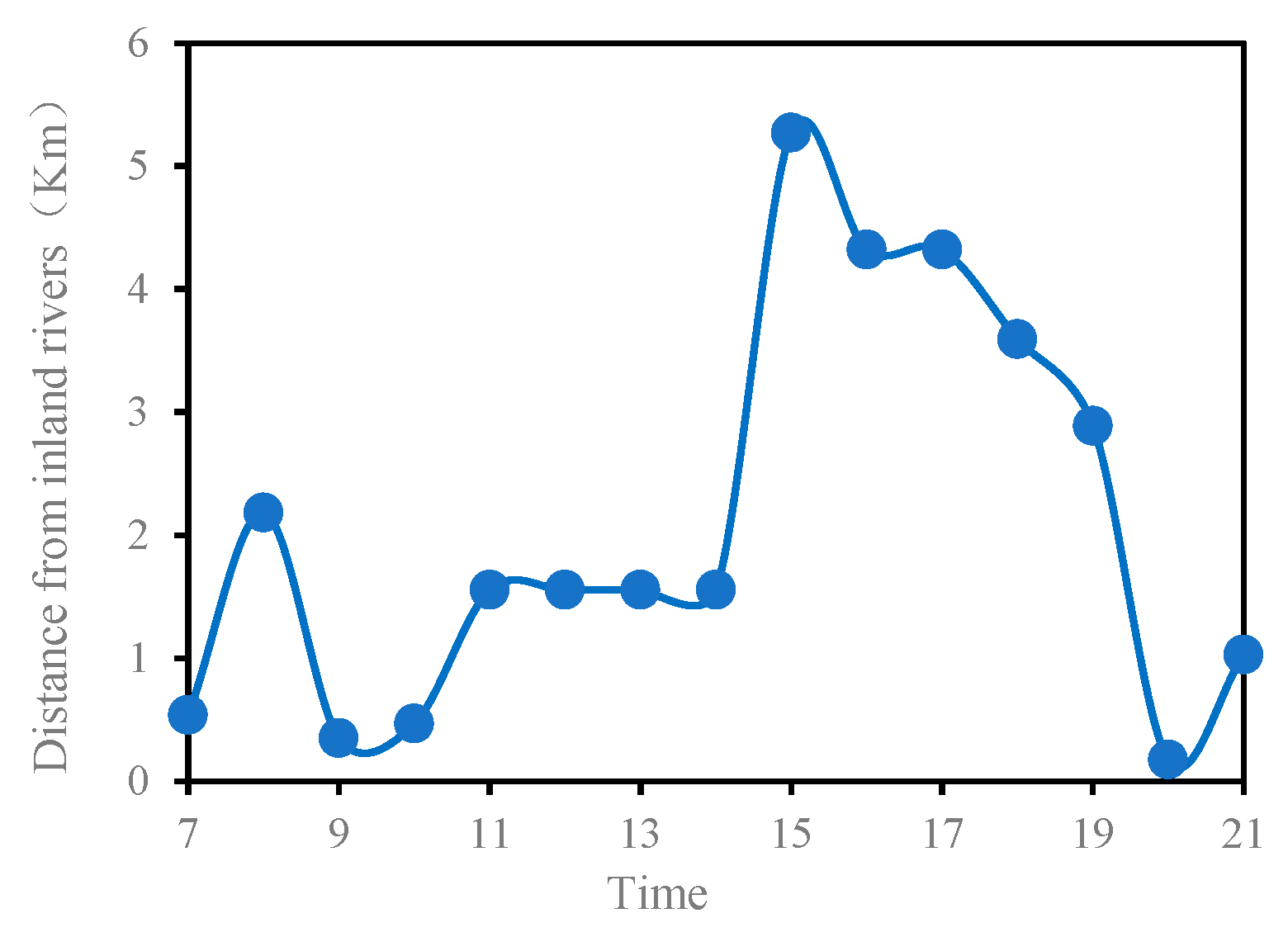
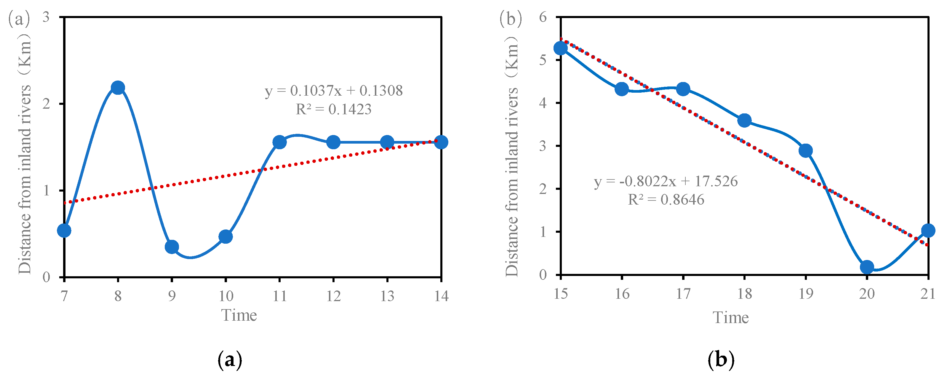
The relationship between the maximum inland penetration of sea breeze cooling, distance to the inland river, and time was analyzed. The results indicate that over the full cooling period (Figure 15), 10 points were situated close to the inland river, specifically between 7:00 and 14:00 and 20:00 and 21:00, matching the spatial distribution analysis based on plan-view maps. In the correlation analysis, the time range from 7:00–14:00 showed a weak positive correlation, with a correlation coefficient of 0.38 (Figure 16a). The time range of 15:00–21:00 showed a strong negative correlation and the correlation coefficient was −0.93 (Figure 16b). Over time, the distance to the inland river decreased.

Figure 15. Temporal variation in the farthest point distance of the sea breeze cooling area from an inland river.

Figure 16. (a) Variation in the distance from an inland river to the farthest point within the sea breeze cooling area over the time period 7:00–14:00; (b) variation in the distance from an inland river to the farthest point within the sea breeze cooling area over the time period 15:00 and 21:00.

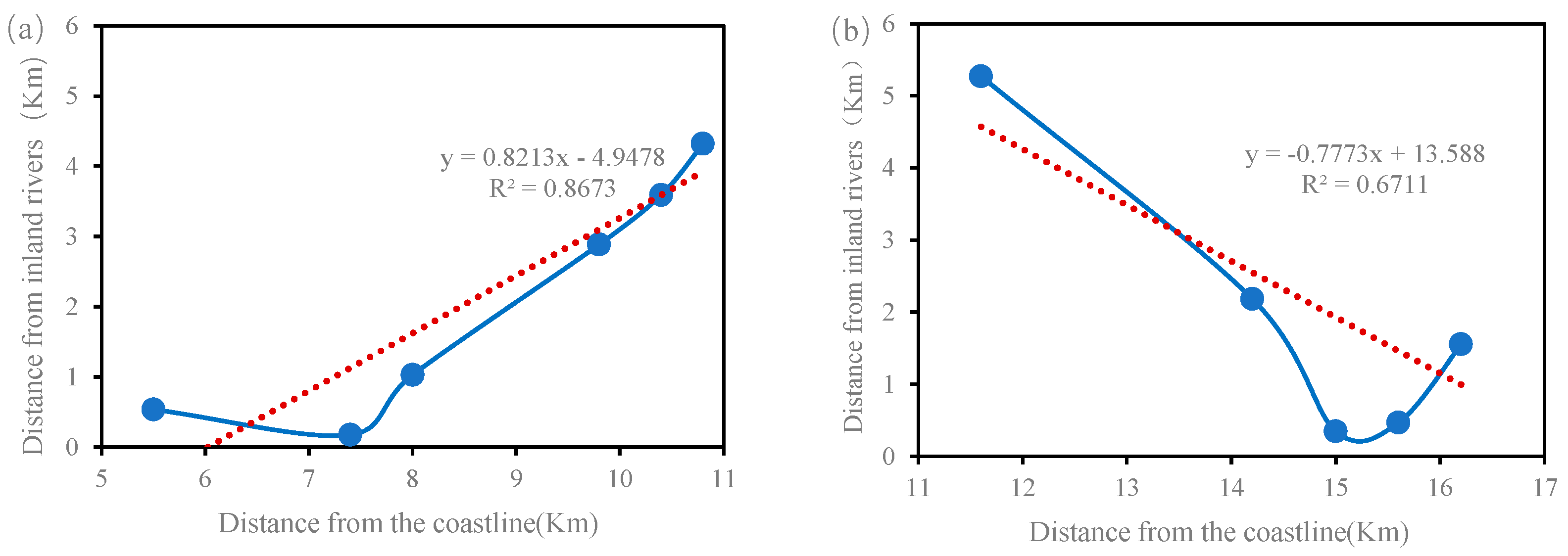
An analysis revealed that when the maximum sea breeze cooling distance fell within the range of 5–11 km, locations farther from the inland river exhibited greater cooling distances (Figure 17a). A strong positive correlation (correlation coefficient = 0.93) was observed between these two factors. In contrast, when the maximum sea breeze cooling distance was between 11 and 17 km, locations closer to the inland river experienced greater cooling distances (Figure 17b). Consequently, when the sea breeze cooling distance exceeded 11 km, points nearer to the inland river exhibited longer cooling distances.

Figure 17. (a) Distance from farthest cooling point to inland river (cooling range: 5–11 km); (b) distance from farthest cooling point to inland river (cooling range: 11–17 km).

Between 8:00 and 15:00, the sea breeze coasters had the longest distance of >11 km. The analysis of the hourly cooling capacity and cooling range showed that 9:00–13:00 had a higher cooling capacity and cooling range. Consequently, it can be inferred that inland rivers play a beneficial role in enhancing sea breeze cooling effects.

6. Conclusions

This study utilized long-term, multi-point observation data to simulate weather conditions in Sendai, Japan, using the WRF model, and visualized the computed Sea Breeze Cooling Capacity (SBCC) for the urban area. A cooling map of SBCC was drawn, the variation trend of cooling capacity per hour was analyzed dynamically, and the factors affecting the SBCC were discussed, as well as the farthest cooling point and inland penetration distance of sea breezes per hour being identified.

This study defines the temperature difference observed between days with sea breezes and days with westerly winds as the cooling capacity of sea breezes in coastal urban areas. The characteristics of the cooling capacity and cooling range of the sea breeze over time were analyzed in detail. The distance between the action point and the coast, the time of the cooling effect, and the inland river were important factors affecting the cooling ability of the sea breeze. The closer the area is to the coast, the stronger the cooling capacity of the sea breeze. From 15:00 to 21:00, with the increase in time, the cooling effect of the sea breeze penetrates to the farthest point of the land, which is closer to the coastline and closer to the inland river. When the farthest distance of sea breeze cooling was within 5–11 km, the distance from the inland river positively correlated with the farthest distance of sea breeze cooling. When the farthest distance of sea breeze cooling was within 11 km to 17 km, the distance from the inland river was negatively correlated with the farthest distance of sea breeze cooling. The area with the strongest cooling capacity per hour was negatively correlated with the time when cooling occurred and the distance from the coast. It was concluded that inland rivers had a positive effect on sea breeze cooling.

Furthermore, this research provides significant insights for promoting urban sustainability. Specifically: (1) Enhancing Climate Resilience: informing the design of urban layouts and ventilation corridors to facilitate sea breeze penetration, thereby reducing urban overheating and improving thermal comfort for residents, which is crucial for adapting to more frequent and intense heatwaves under climate change. (2) Reducing Energy Consumption: by identifying areas with the highest cooling potential, our results can guide strategies to minimize reliance on air conditioning, leading to significant reductions in greenhouse gas emissions from energy production. (3) Supporting Sustainable Urban Planning: the identified positive correlation between inland rivers and enhanced sea breeze cooling underscores the importance of integrating and preserving blue–green infrastructure within urban fabric, which not only boosts natural cooling, but also promotes biodiversity and improves overall urban livability. Consequently, this research aligns with the integrated socio-economic and environmental goals of sustainability by providing a practical tool to define, measure, and monitor the effectiveness of nature-based solutions for sustainable urban development.

References

- IPCC. Climate Change 2014: Synthesis Report. Contribution of Working Groups I, II and III to the Fifth Assessment Report of the Intergovernmental Panel on Climate Change; Pachauri, R.K., Meyer, L.A., Eds.; IPCC: Geneva, Switzerland, 2014; p. 151. [Google Scholar]
- Wang, S.; Zhu, J. Amplified or exaggerated changes in perceived temperature extremes under global warming. Clim. Dyn. 2020, 54, 117–127. [Google Scholar] [CrossRef]
- Woodward, A.; Smith, K.R.; Campbell-Lendrum, D.; Chadee, D.D.; Honda, Y.; Liu, Q.; Haines, A. Climate change and health: On the latest IPCC report. Lancet 2014, 383, 1185–1189. [Google Scholar] [CrossRef]
- Gu, S.; Huang, C.; Bai, L.; Chu, C.; Liu, Q. Heat-related illness in China, summer of 2013. Int. J. Biometeorol. 2016, 60, 131–137. [Google Scholar] [CrossRef] [PubMed]
- Xia, Y.; Li, Y.; Guan, D.; Tinoco, D.M.; Xia, J.; Yan, Z.; Yang, J.; Liu, Q.; Huo, H. Assessment of the economic impacts of heat waves: A case study of Nanjing, China. J. Clean. Prod. 2018, 171, 811–819. [Google Scholar] [CrossRef]
- Li, X.X. Linking residential electricity consumption and outdoor climate in a tropical city. Energy 2018, 157, 734–743. [Google Scholar] [CrossRef]
- Fouillet, A.; Rey, G.; Laurent, F.; Pavillon, G.; Bellec, S.; Guihenneuc-Jouyaux, C.; Hémon, D. Excess mortality related to the August 2003 heat wave in France. Int. Arch. Occup. Environ. Health 2006, 80, 16–24. [Google Scholar] [CrossRef]
- Papathoma-Koehle, M.; Promper, C.; Bojariu, R.; Cica, R.; Sik, A.; Perge, K.; Glade, T. A common methodology for risk assessment and mapping for south-east Europe: An application for heat wave risk in Romania. Nat. Hazards 2016, 82, 89–109. [Google Scholar] [CrossRef]
- Elizabeth Loughnan, M.; Tapper, J.N.; Phan, T.A.; McInnes, J. Can a spatial index of heat-related vulnerability predict emergency service demand in Australian capital cities? Int. J. Emerg. Serv. 2014, 3, 6–33. [Google Scholar] [CrossRef]
- Yang, L.; Niyogi, D.; Tewari, M.; Aliaga, D.; Chen, F.; Tian, F.; Ni, G. Contrasting impacts of urban forms on the future thermal environment: Example of Beijing metropolitan area. Environ. Res. Lett. 2016, 11, 034018. [Google Scholar] [CrossRef]
- Balchin, W.G.V.; Pye, N. A micro-climatological investigation of bath and the surrounding district. Q. J. R. Meteorol. Soc. 1947, 73, 297–323. [Google Scholar] [CrossRef]
- Oke, T.R. The energetic basis of the urban heat island. Q. J. R. Meteorol. Soc. 1982, 108, 1–24. [Google Scholar] [CrossRef]
- Peng, S.; Piao, S.; Ciais, P.; Friedlingstein, P.; Ottle, C.; Bréon, F.M.; Myneni, R.B. Surface urban heat island across 419 global big cities. Environ. Sci. Technol. 2012, 46, 696–703. [Google Scholar] [CrossRef]
- Stewart, I.D.; Oke, T.R. Local climate zones for urban temperature studies. Bull. Am. Meteorol. Soc. 2012, 93, 1879–1900. [Google Scholar] [CrossRef]
- Hogan, A.W.; Ferrick, M.G. Observations in nonurban heat islands. J. Appl. Meteorol. Climatol. 1998, 37, 232–236. [Google Scholar] [CrossRef]
- Kłysik, K.; Fortuniak, K. Temporal and spatial characteristics of the urban heat island of Łódź, Poland. Atmos. Environ. 1999, 33, 3885–3895. [Google Scholar] [CrossRef]
- Morris, C.J.G.; Simmonds, I. Associations between varying magnitudes of the urban heat island and the synoptic climatology in Melbourne, Australia. Int. J. Climatol. J. R. Meteorol. Soc. 2000, 20, 1931–1954. [Google Scholar] [CrossRef]
- Morris, C.J.G.; Simmonds, I.; Plummer, N. Quantification of the influences of wind and cloud on the nocturnal urban heat island of a large city. J. Appl. Meteorol. Climatol. 2001, 40, 169–182. [Google Scholar] [CrossRef]
- Unger, J.; Sümeghy, Z.; Zoboki, J. Temperature cross-section features in an urban area. Atmos. Res. 2001, 58, 117–127. [Google Scholar] [CrossRef]
- Seino, N.; Aoyagi, T.; Tsuguti, H. Numerical simulation of urban impact on precipitation in Tokyo: How does urban temperature rise affect precipitation? Urban Clim. 2018, 23, 8–35. [Google Scholar] [CrossRef]
- Guhathakurta, S.; Gober, P. The impact of the Phoenix urban heat island on residential water use. J. Am. Plan. Assoc. 2007, 73, 317–329. [Google Scholar] [CrossRef]
- Guan, H.; Soebarto, V.; Bennett, J.; Clay, R.; Andrew, R.; Guo, Y.; Bellette, K. Response of office building electricity consumption to urban weather in Adelaide, South Australia. Urban Clim. 2014, 10, 42–55. [Google Scholar] [CrossRef]
- Lapola, D.M.; Braga, D.R.; Di Giulio, G.M.; Torres, R.R.; Vasconcellos, M.P. Heat stress vulnerability and risk at the (super) local scale in six Brazilian capitals. Clim. Change 2019, 154, 477–492. [Google Scholar] [CrossRef]
- Smoyer-Tomic, K.E.; Kuhn, R.; Hudson, A. Heat wave hazards: An overview of heat wave impacts in Canada. Nat. Hazards 2003, 28, 465–486. [Google Scholar] [CrossRef]
- Sun, Z.; Yu, S.; Guo, H.; Wang, C.; Zhang, Z.; Xu, R. Assessing 40 years of spatial dynamics and patterns in megacities along the Belt and Road region using satellite imagery. Int. J. Digit. Earth 2021, 14, 71–87. [Google Scholar] [CrossRef]
- Morabito, M.; Crisci, A.; Gioli, B.; Gualtieri, G.; Toscano, P.; Di Stefano, V.; Orlandini, S.; Gensini, G.F. Urban-hazard risk analysis: Mapping of heat-related risks in the elderly in major Italian cities. PLoS ONE 2015, 10, e0127277. [Google Scholar] [CrossRef]
- Puygrenier, V.; Lohou, F.; Campistron, B.; Saïd, F.; Pigeon, G.; Bénech, B.; Serça, D. Investigation on the fine structure of sea-breeze during ESCOMPTE experiment. Atmos. Res. 2005, 74, 329–353. [Google Scholar] [CrossRef]
- Bouchlaghem, K.; Mansour, F.B.; Elouragini, S. Impact of a sea breeze event on air pollution at the Eastern Tunisian Coast. Atmos. Res. 2007, 86, 162–172. [Google Scholar] [CrossRef]
- Wu, M.; Wu, D.; Fan, Q.; Wang, B.M.; Li, H.W.; Fan, S.J. Observational studies of the meteorological characteristics associated with poor air quality over the Pearl River Delta in China. Atmos. Chem. Phys. 2013, 13, 10755–10766. [Google Scholar] [CrossRef]
- Pattiaratchi, C.; Hegge, B.; Gould, J.; Eliot, I. Impact of sea-breeze activity on nearshore and foreshore processes in southwestern Australia. Cont. Shelf Res. 1997, 17, 1539–1560. [Google Scholar] [CrossRef]
- Freitas, E.D.; Rozoff, C.M.; Cotton, W.R.; Dias, P.L.S. Interactions of an urban heat island and sea-breeze circulations during winter over the metropolitan area of São Paulo, Brazil. Bound.-Layer Meteorol. 2007, 122, 43–65. [Google Scholar] [CrossRef]
- Carter, M.; Shepherd, J.M.; Burian, S.; Jeyachandran, I. Integration of lidar data into a coupled mesoscale-land surface model: A theoretical assessment of sensitivity of urban-coastal mesoscale circulations to urban canopy parameters. J. Atmos. Ocean. Technol. 2012, 29, 328–346. [Google Scholar] [CrossRef]
- He, B.J.; Ding, L.; Prasad, D. Relationships among local-scale urban morphology, urban ventilation, urban heat island and outdoor thermal comfort under sea breeze influence. Sustain. Cities Soc. 2020, 60, 102289. [Google Scholar] [CrossRef]
- Dandou, A.; Tombrou, M.; Soulakellis, N. The influence of the city of Athens on the evolution of the sea-breeze front. Bound.-Layer Meteorol. 2009, 131, 35–51. [Google Scholar] [CrossRef]
- Shen, L.; Zhao, C.; Ma, Z.; Li, Z.; Li, J.; Wang, K. Observed decrease of summer sea-land breeze in Shanghai from 1994 to 2014 and its association with urbanization. Atmos. Res. 2019, 227, 198–209. [Google Scholar] [CrossRef]
- Khan, S.M.; Simpson, R.W. Effect of a heat island on the meteorology of a complex urban airshed. Bound.-Layer Meteorol. 2001, 100, 487–506. [Google Scholar] [CrossRef]
- Fovell, R.G. Convective initiation ahead of the sea-breeze front. Mon. Weather Rev. 2005, 133, 264–278. [Google Scholar] [CrossRef]
- Hu, T.; Wang, Y.; Wu, D. The interaction of an urban heat island with a sea breeze front during moist convection over Tianjing, China. Weather 2022, 77, 238–247. [Google Scholar] [CrossRef]
- Ameer, S.; Shah, M.A.; Khan, A.; Song, H.; Maple, C.; Islam, S.U.; Asghar, M.N. Comparative analysis of machine learning techniques for predicting air quality in smart cities. IEEE Access 2019, 7, 128325–128338. [Google Scholar] [CrossRef]
- Gedzelman, S.D.; Austin, S.; Cermak, R.; Stefano, N.; Partridge, S.; Quesenberry, S.; Robinson, D.A. Mesoscale aspects of the urban heat island around New York City. Theor. Appl. Climatol. 2003, 75, 29–42. [Google Scholar] [CrossRef]
- Lopes, A.; Lopes, S.; Matzarakis, A.; Alcoforado, M.J. The influence of the summer sea breeze on thermal comfort in Funchal (Madeira): A contribution to tourism and urban planning. Meteorol. Z. 2011, 5, 553–564. [Google Scholar] [CrossRef]
- Yang, J.; Xin, J.X.; Zhang, Y.; Xiao, X.M.; Xia, J.C. Contributions of sea-land breeze and local climate zones to daytime and nighttime heat island intensity. npj Urban Sustain. 2022, 2, 12. [Google Scholar] [CrossRef]
- Zhou, Y.; Guan, H.; Huang, C.; Fan, L.; Gharib, S.; Batelaan, O.; Simmons, C. Sea breeze cooling capacity and its influencing factors in a coastal city. Build. Environ. 2019, 166, 106408. [Google Scholar] [CrossRef]
- Guo, F.; Zhao, J.; Zhang, H.; Dong, J.; Zhu, P.; Lau, S.S.Y. Effects of urban form on sea cooling capacity under the heatwave. Sustain. Cities Soc. 2023, 88, 104271. [Google Scholar] [CrossRef]
- Guan, H.; Kumar, V.; Clay, R.; Kent, C.; Bennett, J.; Ewenz, C.; Simmons, C.T. Temporal and spatial patterns of air temperature in a coastal city with a slope base setting. J. Geophys. Res. Atmos. 2016, 121, 5336–5355. [Google Scholar] [CrossRef]
- Kim, Y.H.; Baik, J.J. Daily maximum urban heat island intensity in large cities of Korea. Theor. Appl. Climatol. 2004, 79, 151–164. [Google Scholar] [CrossRef]
- He, B.J. Potentials of meteorological characteristics and synoptic conditions to mitigate urban heat island effects. Urban Clim. 2018, 24, 26–33. [Google Scholar] [CrossRef]
- Zhou, X.; Okaze, T.; Ren, C.; Cai, M.; Ishida, Y.; Watanabe, H.; Mochida, A. Evaluation of urban heat islands using local climate zones and the influence of sea-land breeze. Sustain. Cities Soc. 2020, 55, 102060. [Google Scholar] [CrossRef]
- Yang, Y.; Guo, M.; Wang, L.; Zong, L.; Liu, D.; Zhang, W.; Guo, Y. Unevenly spatiotemporal distribution of urban excess warming in coastal Shanghai megacity, China: Roles of geophysical environment, ventilation and sea breezes. Build. Environ. 2023, 235, 110180. [Google Scholar] [CrossRef]
- Kolokotsa, D.; Psomas, A.; Karapidakis, E. Urban heat island in southern Europe: The case study of Hania, Crete. Sol. Energy 2009, 83, 1871–1883. [Google Scholar] [CrossRef]
- Papanastasiou, D.K.; Melas, D.; Bartzanas, T.; Kittas, C. Temperature, comfort and pollution levels during heat waves and the role of sea breeze. Int. J. Biometeorol. 2010, 54, 307–317. [Google Scholar] [CrossRef] [PubMed]
- Shen, L.; Sun, J.; Yuan, R. Idealized large-eddy simulation study of interaction between urban heat island and sea breeze circulations. Atmos. Res. 2018, 214, 338–347. [Google Scholar] [CrossRef]
- Varquez, A.C.G.; Nakayoshi, M.; Kanda, M. The effects of highly detailed urban roughness parameters on a sea-breeze numerical simulation. Bound.-Layer Meteorol. 2015, 154, 449–469. [Google Scholar] [CrossRef]
- Cenedese, A.; Monti, P. Interaction between an inland urban heat island and a sea-breeze flow: A laboratory study. J. Appl. Meteorol. Climatol. 2003, 42, 1569–1583. [Google Scholar] [CrossRef]
- Thompson, W.T.; Holt, T.; Pullen, J. Investigation of a sea breeze front in an urban environment. Q. J. R. Meteorol. Soc. A J. Atmos. Sci. Appl. Meteorol. Phys. Oceanogr. 2007, 133, 579–594. [Google Scholar] [CrossRef]
- Martilli, A. A two-dimensional numerical study of the impact of a city on atmospheric circulation and pollutant dispersion in a coastal environment. Bound.-Layer Meteorol. 2003, 108, 91–119. [Google Scholar] [CrossRef]
- Sato, T.; Ooka, R.; Murakami, S. The Effect of Building Morphology on Sea Breeze Penetration over the Kanto Plain-Analysis of Mean Kinetic Energy Balance of Moving Control Volume along Sea Breeze. Int. J. High-Rise Build. 2012, 1, 73–80. [Google Scholar] [CrossRef]
- Peng, Z.; Hu, F. A study of the influence of urbanization of Beijing on the boundary wind structure. Chin. J. Geophys. 2006, 49, 1608–1615. [Google Scholar] [CrossRef]
- Gilliam, R.C.; Raman, S.; Niyogi, D.D.S. Observational and numerical study on the influence of large-scale flow direction and coastline shape on sea-breeze evolution. Bound.-Layer Meteorol. 2004, 111, 275–300. [Google Scholar] [CrossRef]
- Gardes, T.; Schoetter, R.; Hidalgo, J.; Long, N.; Marquès, E.; Masson, V. Statistical prediction of the nocturnal urban heat island intensity based on urban morphology and geographical factors-An investigation based on numerical model results for a large ensemble of French cities. Sci. Total Environ. 2020, 737, 139253. [Google Scholar] [CrossRef]
- Al-Ruzouq, R.; Shanableh, A.; Khalil, M.A.; Zeiada, W.; Hamad, K.; Abu Dabous, S.; Jena, R. Spatial and temporal inversion of land surface temperature along coastal cities in Arid Regions. Remote Sens. 2022, 14, 1893. [Google Scholar] [CrossRef]
- Naor, R.; Potchter, O.; Shafir, H.; Alpert, P. An observational study of the summer Mediterranean Sea breeze front penetration into the complex topography of the Jordan Rift Valley. Theor. Appl. Climatol. 2017, 127, 275–284. [Google Scholar] [CrossRef]
- Crosman, E.T.; Horel, J.D. Sea and lake breezes: A review of numerical studies. Bound.-Layer Meteorol. 2010, 137, 1–29. [Google Scholar] [CrossRef]
- Hai, S.; Miao, Y.; Sheng, L.; Wei, L.; Chen, Q. Numerical study on the effect of urbanization and coastal change on sea breeze over Qingdao, China. Atmosphere 2018, 9, 345. [Google Scholar] [CrossRef]
- Kitao, N.; Moriyama, M.; Takebayii, H.; Tanaka, T. A study on making method of climate atlas in Osaka region. AIJ J. Technol. Des. 2012, 18, 255–258. [Google Scholar] [CrossRef]
- He, J.; Chen, D.; Gu, Y.; Jia, H.; Zhong, K.; Kang, Y. Evaluation of planetary boundary layer schemes in WRF model for simulating sea-land breeze in Shanghai, China. Atmos. Res. 2022, 278, 106337. [Google Scholar] [CrossRef]
- Castorrini, A.; Gentile, S.; Geraldi, E.; Bonfiglioli, A. Investigations on offshore wind turbine inflow modelling using numerical weather prediction coupled with local-scale computational fluid dynamics. Renew. Sustain. Energy Rev. 2023, 171, 113008. [Google Scholar] [CrossRef]
- Wong, N.H.; He, Y.; Nguyen, N.S.; Raghavan, S.V.; Martin, M.; Hii, D.J.C.; Deng, J. An integrated multiscale urban microclimate model for the urban thermal environment. Urban Clim. 2021, 35, 100730. [Google Scholar] [CrossRef]
- Zhang, H.; Gong, S.; Zhang, L.; Ni, J.; He, J.; Wang, Y.; Lu, S. Development and application of a street-level meteorology and pollutant tracking system (S-TRACK). Atmos. Chem. Phys. 2022, 22, 2221–2236. [Google Scholar] [CrossRef]
- Fujibe, F. Urban warming in Japanese cities and its relation to climate change monitoring. Int. J. Clim. 2011, 31, 162–173. [Google Scholar] [CrossRef]
- Peng, S.; Kon, Y.; Watanabe, H. Effects of sea breeze on urban areas using computation fluid dynamic—A case study of the range of cooling and humidity effects in sendai, Japan. Sustainability 2022, 14, 1074. [Google Scholar] [CrossRef]
- Powers, J.G.; Klemp, J.B.; Skamarock, W.C.; Davis, C.A.; Dudhia, J.; Gill, D.O.; Duda, M.G. The weather research and forecasting model: Overview, system efforts, and future directions. Bull. Am. Meteorol. Soc. 2017, 98, 1717–1737. [Google Scholar] [CrossRef]
- Skamarock, W.C.; Klemp, J.B.; Dudhia, J.; Gill, D.O.; Barker, D.M. A Description of the Advanced Research WRF Version 3. NCAR Tech; Note NCAR/TN-475+STR; National Center for Atmospheric Research: Boulder, CO, USA, 2008; p. 113. [Google Scholar] [CrossRef]
- Miao, Y.; Liu, S.; Chen, B.; Zhang, B.; Wang, S.; Li, S. Simulating Urban Flow and Dispersion in Beijing by Coupling a CFD Model with the WRF Model. Adv. Atmos. Sci. 2013, 30, 1663–1678. [Google Scholar] [CrossRef]
- Zheng, Y.; Miao, Y.; Liu, S.; Chen, B.; Zheng, H.; Wang, S. Simulating Flow and Dispersion by Using WRF-CFD Coupled Model in a Built-up Area of Shenyang, China. Adv. Meteorol. 2015, 2015, 528618. [Google Scholar] [CrossRef]
- Peng, S.; Watanabe, H. Analysis and mapping of sea breeze event time in coastal cities: A case study of Sendai. Atmosphere 2022, 13, 1484. [Google Scholar] [CrossRef]
- Takebayashi, H.; Tanaka, T.; Moriyama, M.; Watanabe, H.; Miyazaki, H.; Kittaka, K. Relationship between city size, coastal land use, and summer daytime air temperature rise with distance from coast. Climate 2018, 6, 84. [Google Scholar] [CrossRef]
- Sasaki, Y.; Matsuo, K.; Yokoyama, M.; Sasaki, M.; Tanaka, T.; Sadohara, S. Sea breeze effect mapping for mitigating summer urban warming: For making urban environmental climate map of Yokohama and its surrounding area. Urban Clim. 2018, 24, 529–550. [Google Scholar] [CrossRef]
Disclaimer/Publisher’s Note: The statements, opinions and data contained in all publications are solely those of the individual author(s) and contributor(s) and not of MDPI and/or the editor(s). MDPI and/or the editor(s) disclaim responsibility for any injury to people or property resulting from any ideas, methods, instructions or products referred to in the content. |
© 2025 by the authors. Licensee MDPI, Basel, Switzerland. This article is an open access article distributed under the terms and conditions of the Creative Commons Attribution (CC BY) license (https://creativecommons.org/licenses/by/4.0/).