Abstract
As a low-carbon and clean energy source, Coalbed methane (CBM) is of great significance in reducing greenhouse gas emissions, optimizing the energy structure, safeguarding mine safety, and promoting the transformation to a green economy to achieve sustainable development. Coalbed methane (CBM) in Xinjiang’s steeply dipping coal seams is abundant but difficult to predict due to complex geology and distinct gas flow behaviors, making traditional methods ineffective. This study proposes GCN-BiGRU, a parallel dual-module model integrating seepage mechanics, reservoir engineering, geological structures, and production history. The GCN module models wells as nodes, using geological attributes and spatial distances to capture inter-well interference; the BiGRU module extracts temporal dependencies from production sequences. An adaptive fusion mechanism dynamically combines spatiotemporal features for robust prediction. Validated on Baiyanghe block data, the model achieved MAE 59.04, RMSE 94.25, and improved accuracy from 64.47% to 92.8% as training wells increased from 20 to 84. It also showed strong transferability to independent sub-regions, enabling real-time prediction and scenario analysis for CBM development and reservoir management.
1. Introduction
Coalbed methane (CBM) is a crucial component of unconventional natural gas resources [1], and its development offers a triple benefit: energy utilization, enhanced coal mine safety, and environmental protection [2]. Xinjiang stands out as one of China’s fourteen major large-scale coal bases, boasting exceptionally rich CBM resources. Coalbed methane resources in Xinjiang are predicted to reach 9.5 trillion cubic meters (comparable to conventional natural gas resources), accounting for 26% of China’s predicted resources, with huge potential for development [3]. Of the nine gas-bearing basins in China with proven geological reserves of more than 10 trillion cubic meters of natural gas, four are in Xinjiang: the Junggar, Tuha, Tien Shan Series, and Tarim Basins. In recent years, with Xinjiang’s rapid economic and social development, coupled with a global surge in energy demand, accelerating CBM development and utilization has become essential to alleviate energy supply-demand imbalances. Accurate CBM production prediction is fundamental for evaluating reservoir development, optimizing production measures, and judiciously controlling drainage and mining operations [4]. However, in Xinjiang, the complex processes of gas adsorption–desorption, transport mechanisms, and significant well-to-well interference make CBM production prediction particularly challenging. Therefore, developing a rapid and efficient method for CBM production prediction, adapted to actual CBM development conditions, remains a key research priority.
Current research on CBM production forecasting is mainly based on two major methodologies: physical modeling and data-driven. Traditional physical models are typically represented by decline curve analysis (DCA) and numerical simulation. The DCA method establishes empirical equations by fitting historical production curves [5]. However, the unique multi-scale transport mechanism of CBM-involving adsorption, desorption, diffusion, and seepage-differs significantly from that of conventional gas reservoirs. As a result, directly applying the DCA (Decline Curve Analysis) equation for production prediction often leads to substantial deviations, making it difficult to accurately characterize long-term production trends and estimate ultimate recoverable reserves (URR) in CBM wells. Numerical simulation methods overcome some limitations of DCA by constructing multi-field coupled equations. Initially, Seidle and other scholars [6] proposed using conventional black oil simulators to model CBM extraction. As research on CBM storage and transport mechanisms progressed, commercial software modules such as CMG’s GEM and GCOMP of BPAmoco’s were developed to simulate multicomponent flows (CH4, N2, and CO2), though these models notably neglected CBM gas diffusion. In 2003, Shi and Durucan [7,8] developed a dual-diffusion model to describe gas diffusion in low-rank coal matrices, achieving excellent agreement with experimental data. They subsequently applied this model to simulate CO2-enhanced methane recovery. Currently, commercial software packages like CMG and Eclipse can effectively implement these modeling approaches. Zhang et al. [9] developed an IMPES three-dimensional two-phase model, which systematically revealed the interaction between the Langmuir constant and permeability parameters, but the method faces technical bottlenecks in obtaining key parameters: permeability, gas saturation and other core parameters are affected by the dynamic desorption of coal seams and stress-sensitive effects, which are difficult to be accurately measured in real time with the existing detection technology. Consequently, numerical simulation-based CBM production forecasting models exhibit limited predictive accuracy [10].
Artificial intelligence has sped up the use of data-driven methods, which are now better than traditional physical models [11]. These methods find complex patterns directly in the data, avoiding the need for complicated theoretical rules [12]. Their development can be broadly categorized into three stages:
Traditional Machine Learning Stage: early data-driven approaches utilized algorithms such as Multiple Linear Regression (MLR) and Support Vector Regression (SVR) to establish input-output mappings. For example, Albertoni [13] employed MLR to construct a model for evaluating inter-well connectivity, while Guo’s team [14] developed an SVR agent model to achieve yield optimization. However, linear models inherently struggle to capture the complex, nonlinear dynamic features of CBM production.
Integrated learning phase: algorithms such as Random Forest (RF) [15] and Gradient Boosted Decision Tree (GBDT) [16] improve the prediction performance by combining weak learners. Zhu [17] et al. optimized the RF model by combining genetic algorithms and demonstrated the effect of casing pressure on the yield of CBM. Comparative studies such as Ma [18] have shown that the GBDT model significantly outperforms traditional regression methods in dynamic prediction. However, these methods still have limitations when processing intricate time series data.
Deep learning phase: deep learning, with its unique self-training capabilities based on backpropagation (BPNN) algorithms, possesses a stronger ability to capture and learn complex data features [19]. Temporal neural networks, notably, Long Short-Term Memory (LSTM) has effectively addressed time-dependent challenges in yield prediction. Xu et al. [20] combined transfer learning with LSTM to create a transfer-LSTM (T-LSTM), addressing the problem of insufficient samples leading to inadequate model training. Chu et al. [21] combined WA with BiLSTM to construct a WA-BiLSTM model for predicting transient pressure behavior during pressure buildup in underground natural gas storage. More recently, Zhao et al. [22] integrated geological information, spatial information, and time series data to construct a Temporal–Spatial Graph Convolutional Network (TDGCN) model for CBM production prediction, achieving promising results.
In Xinjiang, there are mostly high dip coal seams, and the unique topography of Xinjiang makes the storage state of CBM complex and the physical properties of the reservoir are non-homogeneous. Traditional capacity prediction methods (e.g., numerical simulation, decreasing curve analysis) are limited by the complex geological conditions and non-homogeneous reservoir characteristics, which make it difficult to effectively characterize the temporal and spatial coupling relationship in the dynamic production of CBM wells. In recent years, although deep learning technology has shown significant advantages in the field of CBM development, the existing research focuses on single-dimension or single-factor feature extraction, and fails to fully explore the synergistic mechanism between spatial correlation and temporal dependence in CBM production data. However, the existing research focuses on single dimension or single factor feature extraction. Meanwhile, the single-well prediction method neglects the spatial correlation between production wells, whereas the gas movement is very complex in reality.
According to the above study, the current CBM production prediction faces a double challenge: in the spatial dimension, geological factors such as permeability differences between wells and fracture network connectivity constitute a complex non-Euclidean spatial relationship [23]; in the temporal dimension, the dynamic processes such as drainage depressurization and desorption and diffusion lead to the production showing nonlinear fluctuation characteristics [24].
Inter-well interference is crucial for achieving well-cluster-scale development. It expands the drainage area through pressure superposition, thereby enhancing the desorption rate and increasing the overall gas recovery from the well network. Inter-well interference fundamentally results from the superposition of pressure drop propagation between adjacent wells. This pressure-driven energy migration enhances methane desorption dynamics in coal pores and promotes gas flow through fractures, thereby increasing gas production in the affected wells [25]. Consequently, the spatial proximity between wells significantly influences CBM production prediction. Figure 1 presents a schematic diagram of the inter-well interference mechanism.
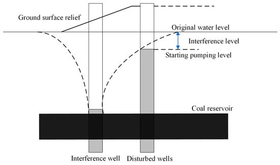
Figure 1.
Schematic diagram of inter-well interference.
To address this problem, this study proposes a GCN-BiGRU parallel fusion architecture that captures spatiotemporal features through dual-channel learning to characterize fluid dynamics, achieving a breakthrough in coalbed methane (CBM) production prediction accuracy. We abstract each production well as a node and construct the topology using inter-well connectivity relationships. To enhance inter-well interference, the layout of coalbed methane (CBM) well patterns is typically irregular and lacks translational invariance, which cannot be characterized by Euclidean spatial data. Graph neural networks (GNNs) excel at processing such non-Euclidean spatial data, as demonstrated in applications like short-term passenger flow prediction and wind speed forecasting. However, establishing adjacency matrices solely based on spatial distance is inadequate, as inter-well interference depends not only on distance but also on reservoir physical properties and geological parameters. Furthermore, these production data constitute time series with complex spatiotemporal correlations. Feng and Jiang [26] developed a gated temporal graph convolutional network (GT-GCN) integrating graph convolution, gated temporal convolution, and residual networks to capture intricate spatiotemporal dependencies. Xiao et al. [27] proposed an AFSTGCN model featuring an adaptive fusion mechanism that simultaneously models temporal, spatial, and spatiotemporal interactions, enabling efficient hierarchical feature extraction and significantly improved prediction performance.
Specifically: (1) The natural/artificial fracture network, a critical flow pathway in coalbed methane (CBM) reservoirs, exhibits strong spatial heterogeneity that fundamentally controls production capacity distribution. To quantify the impact of this spatial structural effect on gas well production prediction, this study constructs a spatial modeling module based on a graph convolutional network (GCN). The approach begins by establishing an initial adjacency matrix using physical distances between wells, then integrating geological attribute similarities to physically represent the fracture network’s potential connectivity structure. Leveraging its information aggregation and transfer mechanism, the GCN enables each node to synthesize neighboring node features, thereby effectively characterizing regional production capacity variations arising from differences in fracture development intensity and topological positioning within the feature space.
(2) To characterize the time-dependent production behavior during CBM development—including adsorption–desorption dynamics, stress-sensitive effects, and other dynamic seepage mechanisms—this study employs a bidirectional gated recurrent unit (BiGRU). Leveraging its bidirectional temporal memory and gated update mechanisms, the BiGRU extracts multi-scale temporal relationships from historical production data, capturing the coupled characteristics of long-term trends and short-term fluctuations. This approach effectively represents the dynamic production patterns evolving with development time.
(3) Adaptive temporal and spatial fusion: the dominant factors governing CBM production—temporal dynamics vs. spatial structure—vary significantly across different development stages (e.g., rapid drainage in the early stage vs. stabilized production in the mid- to late-stage) and across different geologic zones. To address this, an innovative gated fusion mechanism is introduced in this study. Instead of presetting a fixed fusion strategy, this mechanism dynamically learns weights that adaptively assign contribution proportions to the outputs of the temporal state variable (from BiGRU) and the spatial state variable (from GCN). This solution enables accurate modeling of reservoir fluid motion by dynamically balancing the effects of spatial interactions (fracture networks) with temporal evolutionary trends. This integrated spatio-temporal modeling approach ultimately enables more robust and accurate CBM production predictions.
2. Characteristics of Geological Development in the Study Area of Thick Coal Seams with Large Dip Angle in Xinjiang
2.1. Geological Background of Thick Coal Seams with Large Dips
The southern region of the Junggar Basin in Xinjiang is rich in CBM resources, and the coal seams are dominated by low and medium coal rank, which is a key demonstration area for the exploration and development of low coal rank CBM in China [2]. The Fukang Baiyanghe Mining Area is located 100 km east of Urumqi City and 40 km east of Fukang City, covering an area of 15.13 km2. The study area is bounded to the east by the Baiyang River, adjacent to the No. 7 Shaft of the Dahuangshan Coal Mine in Fukang City, and to the west by the Honggou Positive Fault. It is situated in the low mountain-hill zone at the northern foot of Bogda Mountain, on the southeastern edge of the Junggar Basin. The topography of the area is undulating and complex, characterized by numerous ridges and gullies. A prominent ridge, formed by sandstone of the Sanguohe Formation, defines the southern sector of the study region, while flat elevated areas composed of pyroclastic rocks are found in the north. Both the ridges and flat elevated areas align with the regional stratigraphic direction. Topographically, the area is generally higher in the south and lower in the north, with elevations ranging from 1034 to 1338 m, resulting in elevation differences typically around 100 m, and a maximum of 300 m. The northern slopes are steep, predominantly unidirectional, with gradients of 35°–40° and elevation changes of approximately 100 m. In contrast, the southern slopes are less steep, generally comprising several smaller slopes with gradients of 15°–35° and elevation differences between 60 and 100 m. The geographical location map of the study area is presented in Figure 2.
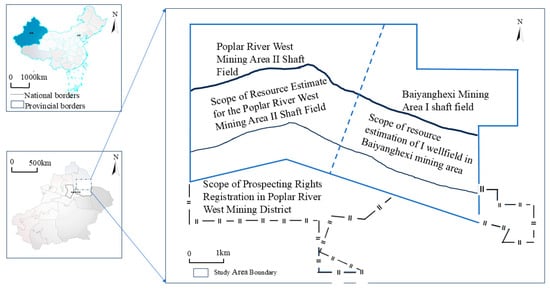
Figure 2.
Geographic location map of the study area.
2.2. Coal Rock Quality and Reservoir Physical Properties
The coal seams in the Fukang mine area are overall shallow in the north and deep in the south in monoclinic [28], and the coal seams within the mining district exhibit a predominant east–west structural trend, with steep dip angles ranging from 45° to 53°. The distribution of wells in the study area is shown in Figure 3a.This geological setting is a result of continuous uplift and extrusion of the Jurassic coal strata, coupled with subsequent denudation of overlying rock layers, primarily influenced by the Yanshanian movements (II and III stages) and the Xishan period movement [29]. According to the tectonic map of the bottom plate of the 42# coal seam (Figure 3b) and the gas content prediction map (Figure 3c), it is estimated that the burial depth of the 42# coal seam in this area is between 0 and 1500 m, and the general direction of the burial line is in an east–west direction. The depth suitable for CBM development is 520−1250 m depth of coal seam (shallow layer is burned by fire).The coal seams are mainly primary structure, the fracture is in jagged shape, the coal body is hard, the fissure is more developed, the average density of face cut is 10 strips/5 cm, maximum reflectance of the specular group averaged 0.59–0.70 %, the coal grade is mainly long-flame coal with lower metamorphic stage, 71.3–96.3% volume fraction of organic matter fraction in microscopic coal rock fractions, and the density of the coal is 1.30−1.41 g/cm3 [30].
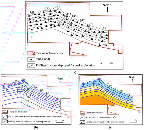
Figure 3.
Basic map of the study area. (a) Map of well locations in the study area (b) Tectonic diagram of the bottom plate of the 42# coal seam [31]. (c) Predicted gas content of 42# coal seam (adapted from literature [31]).
For the seepage of CBM, the main role is played by the cuttings of the coal seam itself, and the pore space plays a small role. According to the preliminary pilot test report of Fukang mine. The face cleats of 41# coal vertical bedding are well developed, with consistent strike, butt cleats are not developed, and the connectivity is poor. The coal rock composition of 42# coal is mainly bright coal and mirror coal. The face cleats of vertical bedding in the coal are well developed, with roughly consistent strike, straight and smooth cleat surface, well-developed butt cleats, intersecting with face cleats at about 80°, with large length variations, partly cutting through face cleats, with continuity, and good to medium connectivity between cleats. The coal rock composition of 44# coal is mainly dark coal, with a small amount of bright coal bands. The face cleats of vertical bedding in dark coal are well developed, with consistent strike, and medium to good connectivity. Compared with coal seams in other regions of China, the permeability of the 41# and 42# coal seams is relatively high, and the reservoir properties of the coal seams demonstrate favorable quality, but there is a strong non-homogeneity.
2.3. Coalbed Methane Storage Characteristics
Coalbed methane is stored in coal seams in three states: free, adsorbed and dissolved, mainly in the adsorbed state, of which more than 90 percent is adsorbed. The main component is methane, which accounts for more than 85−90%. Therefore, the methane adsorption capacity characteristics of coal seams has become an important index for quantitative study of methane storage conditions in coal beds, which can comprehensively reflect the effect of coal rock temperature, pressure, coal quality and other conditions on the methane sorption capacity of coal matrices. According to the theory of CBM adsorption, at constant temperature (T), coal’s methane adsorption capacity follows the Langmuir equation:
where V denotes the adsorption volume at the current pressure; P denotes the gas pressure (MPa); VL denotes the Langmuir volume; PL denotes the Langmuir’s Pressure
Langmuir volume (VL) is an index reflecting the size of coal adsorption capacity, generally speaking, this parameter demonstrates a positive correlation with adsorption capacity; Langmuir pressure serves as a critical parameter governing the curvature characteristics of adsorption isotherms reflecting the adsorption amount of one-half of the Langmuir volume of the pressure when the larger the index, the easier the desorption of adsorbed gases in the coal seam, the more favorable to the development. From the test data (Figure 4), the value of dry air-based Lang’s volume of 44# coal is between 25.33−26.35 m3/t, and the value of dry ash-free base Langmuir volume is between 27.37−27.76 m3/t, reflecting that the coal seam has higher adsorption gas volume. the value of Langmuir’s Pressure of 44# coal is between 1.77−1.79 MPa, reflecting that the coal seam has stronger adsorption capacity.
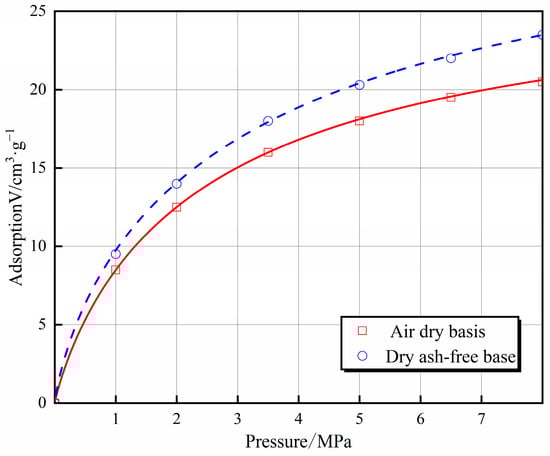
Figure 4.
Isothermal adsorption curve of coal sample.
2.4. Development Characteristics
Production data reveal substantial regional differences in CBM well performance metrics throughout the investigated region, mainly due to different geological features as well as different engineering factors. Field data demonstrate that CBM well production in the investigated region progresses through four characteristic stages: the water production stage, the rising gas production stage, the steady production stage and the decreasing production stage, and the duration of different well types is different. Figure 5 shows the statistics of the highest daily water production and the highest daily gas production in the dataset. The distribution of gas production ranges from 0 to 5120 m3/d, and the distribution of water production ranges from 0 to 110.6 m3/d.
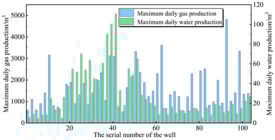
Figure 5.
Statistics of the highest daily production of coalbed methane wells in the Baiyanghe mining area.
Figure 6 shows the typical drainage and production curve of coalbed methane (CBM) wells in steeply dipping coal seams, which evolves through five sequential stages. The process begins with the drainage and pressure reduction stage, where continuous dewatering gradually lowers near-wellbore reservoir pressure below the critical desorption pressure, initiating gas desorption. This transitions into the gas-water coproduction stage, characterized by desorbed gas migrating from coal matrix surfaces into fractures through micropores, with gas-water ratios steadily increasing from low values until peak production is achieved. Following peak production, the system enters a transitional unstable phase marked by significant near-well CBM output and further pressure decline, resulting in pronounced production fluctuations. After this adjustment period, production eventually stabilizes into a steady decline phase, maintaining output levels significantly below peak rates. In steeply dipping coal seams, reservoir heterogeneity—manifesting as higher permeability in the upper sections and lower permeability in the lower sections—combined with gravity effects divides the gas production process into two distinct stages, resulting in a characteristic double-peak production curve. Initially, gas in the upper seam section, which experiences lower geostress, better fracture development, and consequently higher permeability, desorbs and discharges rapidly, forming the first production peak. Subsequently, as drainage continues, the pressure reduction slowly propagates downward into the deeper, low-permeability sections. Due to this lower permeability, it takes significantly longer for the reservoir pressure in these deeper zones to decline to the critical desorption pressure. Once this critical pressure is reached, the vast quantities of adsorbed gas stored within the deeper coal begin to rapidly desorb. This gas then flows preferentially along the dominant fracture direction aligned with the seam dip (strike-dip direction), generating a stronger, but delayed, second production peak [32]. In addition, due to the non-homogeneity of the reservoir and the tectonic complexity of large dip coal beds, the gas production curve may also have multiple peaks. The two or more peaks of gas production in the process of coalbed methane well drainage, on the one hand, is due to the large flow pressure drop in the early stage of drainage, the limited range of reservoir pressure propagation, the large dip angle of the coal seam leads to better connectivity between the main fissure zone and the wellbore, which gives priority to desorption of gas production, and it is difficult to supply gas to the distant part of the reservoir in a timely manner, and on the other hand, it is due to the fact that with the continuation of the drainage, the pressure of the lower coal beds (which are more deeply embedded due to the inclination) is gradually reduced to the critical desorption pressure. On the other hand, as the drainage continues, the pressure of the lower coal seam (due to the greater depth of inclination) gradually decreases to the critical desorption pressure, releasing the closed gas, and the gas output is not synchronous due to the difference in gas content and permeability distribution of different parts of the large inclination reservoir.
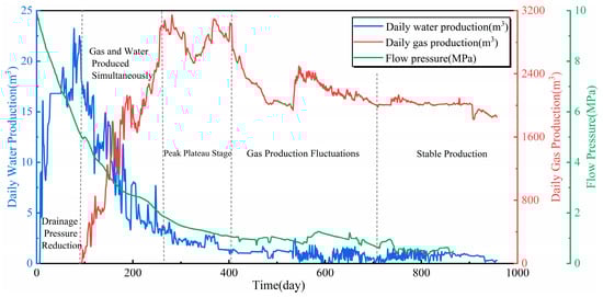
Figure 6.
Typical coalbed methane well discharge and recovery curve.
3. Method
3.1. Overview
In this paper, a deep learning model fusing temporal and spatial features is proposed for CBM production prediction. Before model training, to address the challenge of missing values often encountered in field production data, we employ an XGBoost-based imputation method to ensure data completeness and quality. The core of our GCN-BiGRU architecture consists of two parallel and synergistic branches: a Graph Convolutional Network (GCN) channel and a Bidirectional Gated Recurrent Unit (BiGRU) channel, the GCN branch is designed for spatial feature extraction with particular emphasis on the characterization of high-dip-angle formations and the underlying physics of fluid transport in porous media; meanwhile, the processed dynamic production data from wells are fed into the BiGRU branch for temporal feature extraction, maximize the utility of the bidirectional mechanism to extract the forward and reverse dynamic parameter features, and then fusing the temporal and spatial features through the gating mechanism. Compared to serial architectures (e.g., GCN→BiGRU or BiGRU→GCN), parallel architectures better preserve the inherent strengths of both spatial and temporal features by processing them concurrently, thereby avoiding the dilution of one feature type by another during sequential transfer. This advantage is critical because spatial correlations and temporal dynamics are equally vital yet relatively independent characteristics in CBM production. Furthermore, unlike simple feature concatenation, the parallel architecture integrated with a gating mechanism can adaptively adjust feature weights in accordance with CBM production principles, making it more aligned with the distinct stage characteristics of CBM production. In contrast to the attention mechanism, the gating mechanism achieves efficient and robust feature selection through straightforward linear transformations. This simplicity enhances its applicability in practical scenarios involving large well groups and imperfect data conditions, such as missing or anomalous values. Such comprehensive modeling capability is essential for achieving high-precision CBM production forecasts, particularly in challenging environments characterized by significant spatial heterogeneity and dynamic temporal variations (e.g., large-dip coal seams). These operational steps effectively address the critical challenge of modeling fluid migration patterns within reservoirs, ultimately enabling accurate prediction of CBM production.
3.2. Extreme Gradient Boost (XGBoost)
When deep learning is used for coalbed methane production prediction, the quality, diversity, and completeness of the data directly determine the accuracy and reliability of the models. Real-world recorded data, particularly in complex operational environments like CBM production, frequently suffer from missing values due to interference from various factors such as environmental conditions, sensor malfunctions, and human behavior. These omissions can significantly compromise data quality and impact the accuracy of subsequent analytical models. To address this critical issue, we employed XGBoost (Extreme Gradient Boosting) for missing value imputation. XGBoost is an advanced ensemble learning algorithm introduced by Chen and Guestrin in 2016 [33]. A key advantage of XGBoost is its inherent capability to handle missing values robustly: when constructing decision trees, it automatically treats missing data as a special state and optimally determines the best splitting direction without requiring prior imputation. This approach effectively avoids the bias often introduced by traditional imputation methods (e.g., mean imputation). CBM production is affected not only by time-series factors, but also by other dynamic features. These include daily water production, bottomhole flow pressure, and casing pressure. XGBoost can use the complex relationships in this multi-dimensional data to estimate missing values. This approach provides a more accurate estimate than purely time-series methods, such as interpolation. It is better at handling the interaction of multiple factors. XGBoost excels at accurately capturing these implicit relationships through its multi-tree integration and sophisticated feature combination mechanisms. Its core formulation is based on a gradient boosting framework and optimized using a regularized objective function. This objective function, L(θ), comprises a loss function to quantify prediction error and a regularization term to control decision tree complexity, thereby effectively preventing overfitting. The objective function L(θ) can be written as
where and denote the true and predicted values; denotes the kth decision tree model; γ and λ denote the penalty coefficients; and T and w define the number of leaf nodes and the corresponding weight vectors, respectively.
XGBoost is the stepwise optimization of the objective function by means of an additive model, assuming that the prediction at step is:
Substituting Equations (3) and (4) into (2) and performing a Taylor expansion yields
C is a constant term, and are the first-order and second-order derivatives, respectively, and after simplification, the objective function is
where is the set of samples on leaf node j, and the optimal leaf weights can be obtained by deriving:
3.3. Spatial Feature Extraction
CBM production wells exhibit spatial interdependencies, and the spatial relationship between CBM wells in large inclination terrain is more complicated, the degree of inter-well connectivity reflects both geological spatial characteristics and fluid dynamics variations among production wells. Therefore, it is essential to characterize geological spatial features based on connectivity relationships. Conventional studies predominantly employ convolutional neural networks (CNNs) for spatial feature extraction from structured image data, whereas the distribution pattern of coalbed methane wells inherently constitutes unstructured graph data, and parameters such as permeability, porosity, and fracture distribution of CBM under a large inclined terrain usually have a high degree of spatial non-homogeneity (non-Euclidean structure), so traditional CNNs are not suitable for extracting spatial features of CBM wells under a large inclined terrain features. Graph Convolutional Network (GCN) [34] is a deep learning model based on graph theory. GCN perform information propagation through convolutional operations, where node states are updated by aggregating features from adjacent nodes. This mechanism, known as message passing, enables multi-hop neighborhood information capture through layered propagation. Using GCN for spatial feature extraction can flexibly characterize reservoir features and well deal with the anisotropy of reservoir space due to large dip angles, so that unstructured spatial features can be learned directly to construct the adjacency matrix and well topological relationships that characterize local geospatial information. In order to reduce the computational complexity, the number of GCN layers is set to 2 [35], and the topology between wells is shown in Figure 7. 2-layer GCN model can be expressed as:
where X denotes the identity matrix; A denotes the adjacency matrix; ; ; is a degree matrix; ; and denotes the weighting matrix in the first and second layers; σ and denotes the activation function.
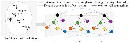
Figure 7.
Inter-well topology.
In this network model, the circular nodes specifically indicate gas production wells. Solid black lines indicate inter-well connectivity. Green dashed lines indicate that neighboring production well points can be reached along the direction of fluid seepage. Orange dashed lines indicate the effect of a well point at one time on the next. Blue dashed lines indicate the long correlation between different time series data for a single well, respectively.
To accurately capture the anisotropy of permeability inherent in large-dip coal seams, we enhance the conventional Euclidean distance by incorporating a burial depth feature when calculating the spatial distance between wells. This modification ensures that the calculated spatial distances more realistically reflect fluid flow paths in such complex geologic environments, and the calculation formula is as follows:
where are the coordinates of well i; is the burial depth of well i; and λ regulates the weight of vertical variance.
Instead of using the traditional binary matrix in this study, a hierarchical map construction method was used to represent the spatial correlation between coalbed methane wells with large inclination angles through weights. Enhancing inter-well interference can effectively increase the production of CBM wells, and neighboring CBM wells tend to exhibit specific production patterns.
Firstly, spatial pre-screening is carried out to construct an initial neighbor matrix, in order to avoid noise interference, this study adopts the K-nearest-neighbor method based on which each node retains only the nearest K neighbors, and the initial neighbor matrix is shown as follows:
where denotes the k nearest neighbors of node i; denotes the connectivity between nodes i and j.
Traditional spatial analysis methods often fall short in accurately depicting the intricate geological spatial features and fluid movement changes between coalbed methane (CBM) production wells because they typically do not consider specific geological characteristics. To overcome this limitation, this study innovatively integrates geological attributes into the construction of the adjacency matrix, creating a more realistic representation of inter-well connectivity and interference in complex large-dip coal seams.
For well A and B, their geological attributes can be quantified through n key parameters, mathematically expressed by:
Building upon the initial neighbor matrix established through spatial pre-screenin, we perform a crucial second step: adjusting edge weights based on the similarity of geological attributes. In this study, the coal seam thickness, gas content and reservoir pressure are selected to form the exact set of attributes of the eigenvector . This process selectively enhances important connections while suppressing irrelevant ones, allowing our graph to more accurately represent the true inter-well interference and fluid flow dynamics in large-inclination CBM reservoirs. The overall graph construction process is visually summarized in Figure 8. A key advantage of this two-step approach is its ability to mitigate issues that arise from purely attribute-based full connectivity. If we were to construct a graph solely on attribute similarity, it could lead to a large number of weakly associated edges (e.g., connecting two nodes that are geographically extremely far apart but happen to have similar attributes by chance). Our hierarchical method ensures that only spatially pre-screened, initially connected wells (i.e., edges where ≠A) have their weights further refined by geological attribute similarity. For these connected edges, we calculate the attribute similarity weight and then apply a correction (the edge of ≠0):
where Sij denotes the attribute similarity between node i and node j; is the geological attribute vector of node i; controls the sensitivity of attribute similarity.
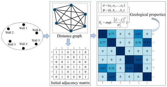
Figure 8.
Methods of construction of graphs.
The Gaussian kernel hyperparameter was tuned using Bayesian optimization. We set its range from 0.1 to 10 and ran the optimization for 30 iterations. The goal was to minimize the mean square error (MSE) on the validation set.
Correcting the adjacency matrix:
3.4. Temporal Feature Extraction
Dynamic production data from coalbed methane wells have significant time dependencies. In recent years, recurrent neural networks (RNNs), with their unique training mechanisms, have shown better application in time series correlation problems. Gated Recurrent Unit (GRU) is a recurrent neural network (RNN) proposed by Cho et al. in 2014 [36]. The GRU architecture fundamentally consists of two gating mechanisms: an update gate (zt) that regulates feature significance for long-term dependency preservation, and a reset gate (rt) that selectively purges irrelevant historical information through memory modulation. Compared to LSTM (3 gating units), GRU requires only 2 gates, which reduces the amounts of parameters by about 33% and provides faster training. The cyclic unit formulation of GRU is as follows:
where denotes the current GRU input value; , , is the weight matrix; is the output of the current position; is the output value from the previous time step; , and are the deviations; and σ are activation functions.
While unidirectional RNNs, such as the standard GRU, are effective in capturing temporal dependencies, their learning is limited to the preceding sequence context. However, the dynamic production of coalbed methane wells often involves intricate temporal relationships where future events or even the overall context of a sequence can influence current behavior (e.g., cumulative pressure effects, well interference patterns). To address this issue, a Bidirectional GRU (BiGRU) combines a normal GRU and a reverse GRU. Its internal structure is shown in Figure 9.
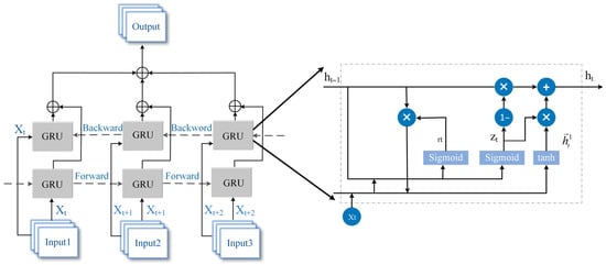
Figure 9.
The internal structure of BiGRU.
We propose the bi-directional gated recurrent unit (BiGRU) model as an improved approach that is capable of extracting multi-scale time dependencies from historical production series and capturing the coupled characteristics of long-term trends and short-term fluctuations. The model consists of two independent GRUs running in parallel. One GRU processes the input data in the forward direction (past to future), capturing dependencies from past states. Meanwhile, the other GRUs processes the data in the reverse direction (future to past), effectively capturing information from future context. This significantly enhances its ability to understand and estimate complex patterns within the sequences [37]. The detailed architecture of the BiGRU network is illustrated in Figure 10.
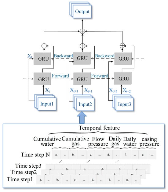
Figure 10.
Detailed structure of the BiGRU network.
3.5. Door Control Fusion
Owing to structural complexity in high-angle stratigraphic configurations, inter-well connectivity and anisotropy are strong. Therefore, different weights need to be assigned to the fused spatio-temporal features to enhance feature processing in important areas. Instead of using a fixed fusion strategy, this mechanism dynamically weights the contributions of the temporal state features (from BiGRU) and spatial state features (from GCN, primarily characterizing fracture network structure) through learnable gating weights (, ).This design computationally adapts to the shifting dominance between physical drivers—such as temporally driven processes during initial drainage and spatially dominated flow in fracture zones—enabling intelligent modeling of dynamic reservoir behaviors.
The data flow within this gated fusion module is controlled by a gating component, which dynamically learns the relative importance of the temporal and spatial features. This component regulates the degree of fusion by determining adaptive weights for each feature, effectively acting as a data-driven switch. and dynamically learn the temporal and spatial features , through the weighting matrix. The training propagation method for the gated fusion module is as follows [38]:
where and are the weight matrix of the temporal gating component and the spatial gating component; and are the output of the temporal and spatial modules; and are the corresponding door assembly; δ(·) is Layer normal; σ(·) is sigmoid; is the output of the gated fusion.
4. Production Forecasting Models
4.1. Model Geology, Development Parameter Settings
Table 1 presents the statistical characterization of both geological parameters and dynamic production data. A total of 105 producing wells with more than 10 years of development were collected. Several characteristics that are closely related to CBM production are flow pressure, casing pressure, daily water production, daily gas production, cumulative water production, cumulative gas production. The spatial distribution of CBM wells is shown in Figure 10.

Table 1.
Static and dynamic production statistics.
The GCN branch requires an input spatial adjacency matrix. Following the spatial feature extraction methodology described in Section 2.3, we first calculate the Euclidean distances between wells based on their spatial coordinates and construct an initial adjacency matrix using the k-nearest neighbors (k-NN) principle. In this binary matrix, neighboring wells are assigned a value of 1 while non-neighboring wells are assigned 0. Subsequently, we incorporate geological attributes (e.g., permeability, gas content) to compute inter-well similarity coefficients Sij, which are used to refine the adjacency matrix. Figure 11 shows some of the wells adjacencies in the study area, where the blue triangles are wells and the brown lines indicate spatial proximity, with corresponding weighting relationships between different wells based on the above calculations.
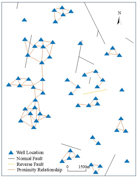
Figure 11.
Study Area Well Neighborhood Map (partial).
4.2. Bayesian Hyperparameter Optimization
Hyperparameters are important factors affecting the accuracy of machine learning, and traditional optimization methods include grid search [39], empirical methods and stochastic search [40]. Grid search is to traverse a predefined combination of hyperparameters and evaluate the performance of the model one by one, which is too computationally expensive. Stochastic search is evaluated by randomly sampling a certain number of combinations from the parameter space, but it is easy to miss the optimal solution when the sampling is insufficient. Bayesian search [41] can automatically capture the nonlinear relationship between parameters and is well suited for this study. It intelligently selects the next evaluation point by constructing a probabilistic agent model (e.g., a Gaussian process) of the objective function with a capture function. The results of optimizing XGBoost using Bayesian hyperparameters in this study are shown in Table 2.
Table 2.
Bayesian hyperparameter optimization.
4.3. Time Window Division
The production dataset is divided into training set wells and test set wells according to 8:2, and the sliding window method is used to partition the data into data of the same length as follows:
where is the time series from time j; is the production data of well i at time j; m is the length of the time window, and n is the step size, which is set to 1.
4.4. Modeling Workflow
The complete experimental workflow, as illustrated in Figure 12, firstly, XGBoost in Section 2.2 was used to fill in the missing values of the dynamic production data in CBM, and the processed data were divided into training set wells and test set wells by wells, based on which the GCN-BiGRU based CBM production prediction model was constructed, and using the coefficient of determination (R2), the root-mean-square error (RMSE) and the Mean Absolute Error (MAE) for K-fold cross-validation of the accuracy of its prediction.
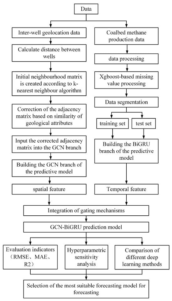
Figure 12.
Model flow chart.
Firstly, the collected dynamic production data are processed, and the XGBoost method in Section 2.2 is used to fill in the missing values, and Bayesian in Section 3.2 is used for hyper-parameter optimization.
Given the complex geological structure, strong inter-well connectivity, and anisotropy inherent in CBM reservoirs, a Graph Convolutional Network (GCN) branch is employed to effectively capture and extract spatial features and inter-well relationships. In the GCN branch, the distances between wells in the training set are first calculated, and the initial neighbor matrix is constructed by screening neighbors based on the calculated distance matrix using the K-nearest-neighbor method, followed by adjusting the edge weights through the similarity of geological attributes and correcting the neighbor matrix, so as to determine the final neighbor matrix, which will provide high-quality inputs for the feature extraction in the GCN. In the testing phase, the mean and variance of the training set are used in the standardization of the test set as a way to ensure that the model handles the test wells in a way that is consistent with the training wells, after which the distance between the wells on the test set and the wells on the training set is recalculated and the neighborhood matrix is rebuilt according to the above method.
Dynamic production data (flow pressure, casing pressure, daily gas production, daily water production) are divided into time windows and entered into another branch BiGRU to capture their intricate temporal dependencies.
Finally, to fully leverage both the extracted spatial and temporal features, a novel gated fusion mechanism is employed. The module adaptively assigns different weights to features from different modalities based on the learned importance, thus enhancing the feature processing in important regions. The overall model prediction process is shown in Figure 13.
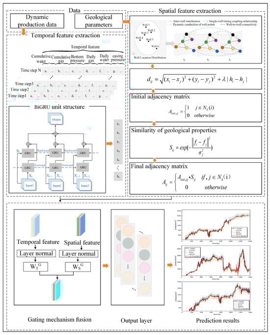
Figure 13.
Intelligent forecasting process of CBM production.
4.5. Evaluation Indicators
During the training process, the mean square error loss (MSE Loss) is used to calculate the error between the predicted and true values as shown in Equation (21):
where and are the true and predicted values, respectively.
To measure the performance of the model, three evaluation metrics, MAE, RMSE, and R2, were used in this study.
- (1)
- Root mean square error (RMSE):
- (2)
- Mean absolute error (MAE):
- (3)
- Coefficient of determination (R2):
5. Analysis of Experimental Results
In this section, six experiments are conducted to validate the performance of the GCN-BiGRU model in coalbed methane production prediction.
Experiment 1 verified the necessity of each component of the model item by item through ablation experiments to demonstrate the contribution of each component to the prediction performance. Experiment 2 compared this model with common machine learning models, highlighting the superior performance of the model proposed in this study in handling the complex spatio-temporal dynamics of CBM production. Experiment 3 analyzed the effect of different well numbers on the model performance. Experiment 4 verified the portability of the model by dividing the data into two independent subregions, I and II. Experimental 5 systematically investigated the impact of hyperparameter variations on model performance metrics, thereby enabling the selection of optimal parameters for the proposed model. Experiment 6 compared the traditional single-well CBM production prediction method with the proposed GCN-BiGRU model, highlighting the latter’s advantages in multi-well joint prediction.
All experiments were run on a computer with these specifications: Windows 11, an Intel Core i7−11850 H CPU, an NVIDIA T600 GPU (NVIDIA, Santa Clara, CA, USA), and 32 GB of RAM. The code used Python 3.12.9 and the PyTorch framework (2.5.1), along with other packages including Pandas 2.2.3 and NumPy 1.26.4 for data processing.
5.1. Ablation Experiment
In this experiment, several models were established for ablation experiments, namely GCN, BiGRU, GCN-BiGRU (string) and GCN-BiGRU, and the same hyperparameter settings were used in all experiments in order to ensure the fairness of the experiments.
A comparison of the predictive performance of each model is shown in Table 3 and Figure 14, respectively, from which it can be seen that each component of the model is necessary and analyzed as follows.
Table 3.
Comparison of predictive performance of each component.
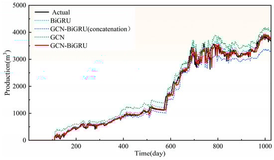
Figure 14.
Comparison of prediction accuracy of GCN-BiGRU components.
- (1)
- Coalbed methane (CBM) production can be effectively improved by controlling factors such as bottom-hole flowing pressure and casing pressure. These factors exhibit complex temporal dependencies. To effectively capture these features and the intrinsic temporal autocorrelation in CBM production data, we employ a bidirectional gated recurrent unit (BiGRU). This model concurrently processes temporal dependencies in both directions: it captures cumulative decline trends through backward propagation while identifying precursor signals of cyclical fluctuations via forward propagation, thereby dynamically extracting time-varying patterns. For instance, when the input sequence shows sustained water production increases (drainage signals), the model reduces future gas production forecasts—a response consistent with actual reservoir dynamics. As corroborated by the improved MAE and RMSE values presented in Table 3, the integration of BiGRU significantly enhances the model’s ability to learn and predict sequential patterns, demonstrating its effectiveness in simulating the temporal dynamics of CBM production.
- (2)
- The spatial feature extraction via GCN enhances CBM production prediction accuracy. By modeling spatial relationships among steeply dipping CBM wells using graph structures, GCN captures non-Euclidean features such as inter-well interference and fracture network connectivity. The model assigns higher weights to neighboring wells exhibiting both spatial proximity and geological similarity. This validates GCN’s capability to identify critical spatial connectivity and reservoir heterogeneity, essential factors in efficient CBM development.
- (3)
- The parallel structure allows for superior model performance. Compared to the serial structure, the parallel structure is designed to allow the model to learn higher-order nonlinear relationships from spatial maps and time series, respectively, and then to model spatio-temporal interactions through a feature fusion layer. As can also be seen from the comparisons in the table, the MAE of the parallel structure is 29.42 lower than that of the serial structure, and the RMSE is 16.44 lower. This enhanced expressiveness underscores the superiority of the parallel architecture over both single networks and sequential designs for robust spatio-temporal CBM production forecasting.
- (4)
- Ablation study results in Table 3 confirm that both spatial and temporal features are critical for accurate CBM production forecasting. When removing BiGRU and relying solely on spatial information, RMSE increased by 195.55 (207%) and MAE by 136.98 (231%). Conversely, excluding GCN and retaining only temporal features elevated RMSE by 35.15 (37%) and MAE by 22.97 (39%). These significant error increments validate the indispensable contributions of both feature types, while the complete integrated model ultimately establishes performance superiority through effective spatiotemporal fusion.
- (5)
- The model structure deliberately allocates component focus to specific physical processes: BiGRU captures complex temporal dynamics driven by adsorption–desorption kinetics coupled with stress sensitivity, while GCN explicitly models regional heterogeneity arising from evolving fracture network topologies. Their integration via gated fusion demonstrates physics-consistent behavior: During early drainage phases, temporal weights dominate (reflecting rapid pressure-driven desorption), whereas fracture-developed zones exhibit significantly enhanced spatial weighting—validating the model’s recognition of fracture connectivity as the governing transport mechanism. This adaptive alignment with reservoir physics not only enhances prediction robustness but provides interpretable physical foundations for model outputs.
5.2. Comprehensive Analysis of Coalbed Methane Production Forecast Models
In this experiment, GCN-BiGRU is compared with classical machine learning models to verify the prediction performance of GCN-BiGRU models. These models include LSTM, BPNN and RNN.
Identical training and testing datasets are maintained throughout all experimental trials, with consistent hyperparameter configurations across each experiment. Table 4 demonstrates the performance of each model.
Table 4.
Prediction capability comparison of different algorithms.
As demonstrated in Table 4, the proposed GCN-BiGRU model delivers more accurate predictions, characterized by significantly lower MAE and RMSE values compared to other benchmark models. In the experiment, four wells on the test set were randomly selected and plotted in Figure 15, from which it can be seen that most of the models follow the overall law of gas production, and GCN-BiGRU fits better than the other models in details. RNNs suffer from the vanishing gradient problem that hinders long-term dependency learning, along with an inherent defect of error accumulation over time steps. The LSTM model exclusively focuses on modeling temporal dependencies in the data, and does not take into account the reservoir. The spatial correlation of the data, such as inter-well interference of neighboring wells, network fracture connectivity. BPNN is unable to deal with dynamic sequences while processing the data; therefore, the other methods are weaker than the GCN-BiGRU proposed in this study. The MAE and RMSE of the GCN-BiGRU reached the best among all the comparisons.
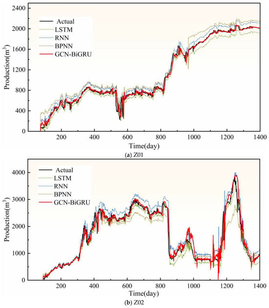
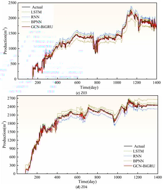
Figure 15.
Plot of yield prediction results for different algorithms.
The anisotropy and spatial characteristics of large dip coal seam reservoirs are a major factor affecting the prediction results, and one of the GCN-BiGRU uses GCN to construct a graph structure to extract the anisotropy features. In order to better describe the inter-well connectivity and fluid movement in large dip coal beds, GCN-BiGRU uses GCN to construct a graph structure to extract anisotropic features.
In terms of temporal feature extraction, the GCN-BiGRU model adopts BiGRU to portray the autocorrelation of data, which fully captures the characteristics of the production data of large-dip coalbed methane wells, and the whole model is also able to more accurately identify the peaks and valleys of the gas production curve. The gating component of the GCN-BiGRU model can dynamically learn features at different stages and adaptively assign different spatio-temporal feature weights. The efficacy of the GCN-BiGRU model’s predictions is further supported by the scatter plot in Figure 16, which visually demonstrates the strong correlation between real and predicted values.
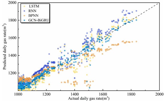
Figure 16.
Scatter plot of predicted versus true values for different algorithms.
5.3. Effect of Number of Wells on Model Performance
In addition to prediction accuracy, it is important to understand how the number of wells affects model performance, given the economic and engineering implications. In this study, well groups were selected using spatial stratified random sampling to ensure even distribution across the study area and coverage of major geological units. First, the area was divided into a 4 × 4 grid (each cell approximately 1 km × 1 km), resulting in 16 subunits. Sample wells were then randomly chosen from each subunit in proportion to its well density, so that the selected wells reflect the actual distribution. During sampling, we ensured that the wells represented all major geological units and were not concentrated in only a few local areas.
This experiment compares four well group configurations: Group A 25 wells(The training set comprises 20 wells, while the test set contains 5 wells), Group B 55 wells(The training set comprises 44 wells, while the test set contains 11 wells), Group C 85 wells(The training set comprises 68 wells, while the test set contains 17 wells), and Group D 105 wells(The training set comprises 84 wells, while the test set contains 21 wells). Results demonstrate substantial prediction accuracy improvements with increasing well density within a critical threshold.
The experimental results show that the improvement of the model performance not only depends on the number of wells, but is also closely related to the spatial coverage integrity of the wells. As Figure 17 illustrates, the 25-well group exhibits poor model fitting and low accuracy (64.47%) due to sparse graph structures that inadequately capture spatial correlations. When well count increases to 85, accuracy rises to 88.43% (Table 5). This is because the additional wells cover more geologic units, enhancing the ability of the GCN module to learn complex spatial relationships between wells. This transition alleviates data scarcity, enabling effective extraction of complex spatial relationships—including inter-well interference and reservoir pressure dynamics.
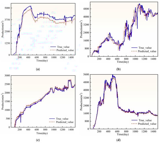
Figure 17.
Plot of predicted results for different numbers of wells. (a) Number of wells is 25; (b) number of wells is 55; (c) number of wells is 85; (d) number of wells is 105.
Table 5.
Comparison of prediction results for different numbers of wells.
Further increasing to 105 wells achieves 92.8% accuracy, but reveals diminishing marginal returns: each additional well yields progressively smaller performance gains. This is due to the fact that most of the additional wells are located in areas that are already densely populated and have limited gain in overall spatial coverage. Beyond optimal well density, continued expansion may cause minimal improvement or even metric fluctuations, indicating model saturation of key spatiotemporal patterns. This suggests additional wells provide limited new information and could potentially introduce noise that degrades model performance.
5.4. Model Portability Validation
This experiment primarily validates model transferability by utilizing existing reservoir blocks divided into two geologically distinct sub-zones (Zone I and Zone II, see Figure 18). We trained the model on Zone I data and tested it on Zone II, simulating generalization from known development areas to new geologically differentiated regions.
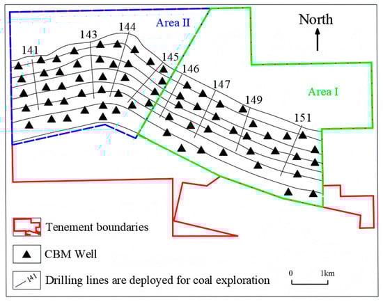
Figure 18.
Study area delineation map.
Figure 19 presents fitted results for two randomly selected test wells in Zone II, with model MAE and RMSE values of 80.9 and 113.34, respectively. Although predictive performance degrades compared to full-block applications, results remain within acceptable thresholds and provide operationally valuable forecasts. Performance deterioration primarily occurs near Zone II’s fault-developed zones, where elevated prediction errors correlate with unmodeled geological complexities. Specifically, heterogeneous fracture network topologies and fault activity characteristics—inadequately represented in Zone I training data—contribute to these localized inaccuracies.
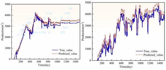
Figure 19.
Yield prediction results for test wells in Zone II.
The model’s strength derives from its data-driven architecture and explicit structural mapping of core physical processes—particularly spatial connectivity and adsorption–desorption temporal dynamics. This enables adaptation to geologically distinct regions sharing similar governing physical mechanisms. For future generalization across basins with more diverse geological settings, acquiring limited datasets from new target blocks will be essential to either fine-tune transfer learning frameworks or integrate region-specific features.
5.5. Impact of Hyperparameters
Hyperparameters are vital in deep learning models, directly influencing their internal architecture, computational efficiency, and ultimately, predictive accuracy. Many studies have shown that learning rate, batch size are two key factors, learning rate ∈ {0.01, 0.005, 0.001, 0.0005, 0.0001} and batch size ∈ {8, 16, 32, 64, 128}. The impact of these parameters on model performance, evaluated using K-fold cross-validation, is meticulously detailed through the box plots presented in Figure 20. This figure visually elucidates the sensitivity of the model’s performance (quantified by MAE and RMSE) to variations in these hyperparameters).
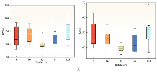
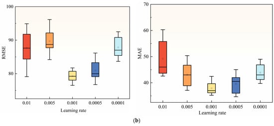
Figure 20.
Sensitivity analysis of hyperparameters. (a) Batch hyperparametric analysis. (b) Hyperparametric analysis of learning rates.
From the plots as the learning rate decreases, the model error shows proportional reduction until converging to its global minimum when the learning rate is 0.001, as quantified by performance metrics, consequently, the learning rate is empirically determined as 0.001 and the MAE and RMSE reaches a minimum when the batch size is 32; therefore, a batch size of 32 is adopted throughout the experiments.
5.6. Performance Evaluation of Gcn-Bigru Versus Conventional Single-Well Prediction Methods
This experiment compares the proposed GCN-BiGRU model with conventional single-well CBM production prediction methods (numerical simulation and decline curve analysis) to demonstrate its superiority.
Numerical simulation methods involve developing mathematical models that describe gas-water flow in porous media. These models simulate reservoir dynamics by solving systems of partial differential equations, typically implemented using commercial simulators such as CMG or Eclipse, or specialized reservoir simulation software.
Decline curve analysis (DCA) extrapolates future production by fitting empirical or semi-empirical decline functions (e.g., Arps hyperbolic decline) to historical production data. This method is widely used for initial reserve assessment and short-to-medium-term production forecasting in oil and gas fields.
Figure 21 demonstrates the fitting performance of GCN-BiGRU versus traditional methods, showing that GCN-BiGRU more accurately fits actual production curves. The GCN module learns spatial topologies of well groups through graph structures to quantitatively characterize drainage-depressurization synergy, while the BiGRU module dynamically deciphers temporal patterns in historical production data. This multi-well joint prediction successfully quantifies the core geo-engineering factor of inter-well interference.
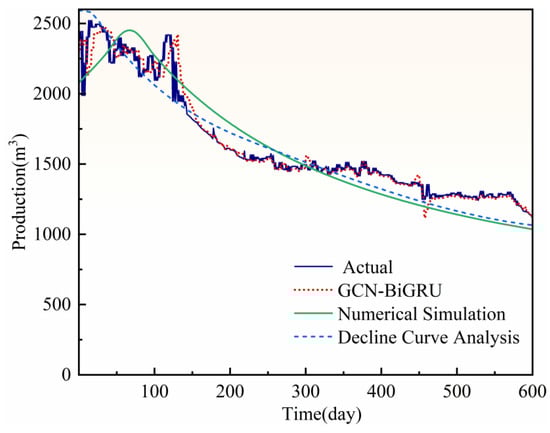
Figure 21.
Prediction Results of GCN-BiGRU vs. Conventional Methods.
In contrast, numerical simulations use idealized reservoir parameters while ignoring dynamic inter-well interference, leading to suboptimal predictions. Decline curve analysis (DCA) exhibits four fundamental limitations: (1) reliance on statistically extrapolated trends lacking physical basis, (2) requirement for stable decline-phase production, (3) poor adaptability to heterogeneous wells (e.g., steeply dipping coal seams), and (4) high uncertainty in long-term forecasts—collectively resulting in unsatisfactory performance.
The model’s superiority is further validated by the evaluation metric results in Figure 22. These results suggest that dynamic disturbances within the inter-well fracture networks may be a primary driver of production fluctuations. Traditional single-well models fail to address well-cluster development scenarios due to their neglect of spatial correlations. In contrast, our framework explicitly models inter-well relationships through graph convolutional networks (GCN) coupled with bidirectional gated recurrent units (BiGRU) to capture temporal nonlinearities, establishing a new paradigm for production prediction under complex geological conditions. Additionally, numerical simulation requires extensive computational time per run, with history matching often demanding hundreds to thousands of iterations. Conversely, once trained, our model achieves real-time prediction speeds suitable for rapid scenario analysis—particularly advantageous for data-rich environments or applications requiring swift deployment.
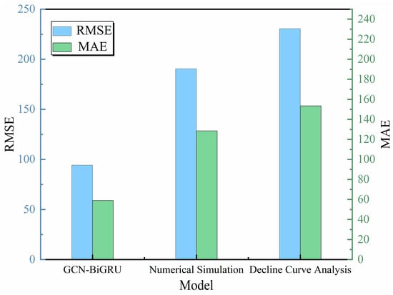
Figure 22.
Comparison of evaluation indicators between GCN-BiGRU and traditional methods.
5.7. Discussion
The GCN-BiGRU model proposed in this study, which integrates the spatial correlation capture capability of graph convolution with the temporal dynamic modeling ability of bidirectional gated recurrent units, demonstrates high prediction accuracy in coalbed methane (CBM) production forecasting. From a sustainability perspective, as a clean energy source, the environmental and economic impacts of CBM cannot be overlooked throughout its life cycle. During the extraction phase, drilling and fracturing generate certain greenhouse gas emissions, and methane leakage significantly increases carbon equivalent emissions. Subsequent transportation, treatment, and purification also entail energy consumption and corresponding emissions. However, when utilized effectively—such as for power generation or as an industrial fuel—CBM can reduce carbon dioxide and other greenhouse gas emissions compared to traditional fossil fuels like coal, offering emission reduction potential. Accurate production forecasting with the GCN-BiGRU model enables more rational planning of extraction intensity and scale, thereby reducing methane leakage and optimizing the emission life cycle. Economically, CBM development involves not only single-well productivity and cost recovery but also resource utilization efficiency and regional energy structure optimization. Reliable production forecasts assist enterprises in operational planning, improving extraction efficiency, reducing unit costs, aligning mining activities with market demand, and stabilizing revenue. Furthermore, as a transitional clean energy source, the sustainable development and utilization of CBM can facilitate the transition to a low-carbon energy structure, deliver long-term economic and environmental synergies, and promote the sustainable development of the energy industry.
The prediction model presented in this study not only improves the accuracy of CBM production forecasts in research, but also offers practical benefits for engineers and operators. For engineers, it supports better well placement and production planning by providing reliable data. This helps optimize resources and reduce exploration risks. For operators, the model enables real-time monitoring and early warnings in daily operations. By detecting production trends early, it guides adjustments in pumping parameters and strategies, helping to prevent abnormal or low-efficiency wells. In this way, the model improves prediction accuracy while also enhancing the safety, cost-effectiveness, and sustainability of field operations.
The GCN-BiGRU model presented in this study shows clear advantages in predicting coalbed methane production, as confirmed through experiments. It can also support mine production planning and sustainable development. However, from both engineering and academic perspectives, the model still has some limitations. Future research should focus on improving it in the following areas:
The GCN-BiGRU model proposed in this study demonstrates significant advantages in coalbed methane (CBM) production prediction through comparative experiments. However, the following potential limitations warrant further investigation:
Partitioned block experiments reveal performance degradation in the model, indicating a need to enhance its generalization capability. Future work should incorporate graph structure enhancement techniques to construct multi-scale graph convolutions for capturing heterogeneous fracture networks.
Given the critical importance of accurate water production prediction for drainage management and production optimization in CBM wells, this study will extend the model’s capabilities in future work. While the current framework focuses on gas production-related spatiotemporal patterns (e.g., adsorption–desorption dynamics and fracture-matrix flow), water production behavior—particularly during early development stages—is governed by two-phase gas-water seepage mechanisms distinct from gas-dominated flow regimes. Future research will develop multi-output architectures to achieve synergistic high-precision prediction of both gas and water production profiles.
Although the model structure maps physical systems, its internal prediction logic lacks the physical transparency of equation-based methods compared to physics-based numerical simulations. Future integration of physical mechanisms with deep learning will enhance model interpretability and robustness.
6. Conclusions
This study proposes a novel GCN-BiGRU deep learning model for coalbed methane production prediction with the large inclined terrain in Xinjiang as the research background, for which a series of experiments have been carried out and the following conclusions have been drawn:
- (1)
- All components in the GCN-BiGRU model gave positive effects to the whole model, with only 59.04 and 94.25 MAE and RMSE, which significantly improved the accuracy of the prediction and verified the reasonableness of the model.
- (2)
- When extracting spatial features, this study proposes integrating geological factors into adjacency matrix construction. This approach effectively characterizes production heterogeneity in steeply dipping coal seams, capturing the combined effects of geological structures, stress distributions, and seepage conditions. Consequently, it enhances the model’s capability to represent complex nonlinear spatial relationships.
- (3)
- The effect of the number of wells on the model performance was analyzed, and the accuracy of the model prediction also increased from 64.47% to 92.8% when the number of wells in the training sample well set increased from 20 to 84 wells.
- (4)
- To evaluate model portability, we partitioned the entire reservoir block into geologically distinct Zones I and II. The model achieved MAE and RMSE values of 80.9 and 113.34, respectively, on the independent test zone. Although performance metrics show degradation compared to whole-block predictions, results remain within acceptable operational thresholds while providing valuable predictive insights. This demonstrates the methodology’s robustness and applicability across heterogeneous reservoir segments.
- (5)
- Comparing and analyzing GCN-BiGRU with the traditional single-well prediction method, the model shows good prediction accuracy, and compared with the traditional method GCN-BiGRU is able to satisfy the demand of real-time prediction and fast scene analysis.
Author Contributions
Conceptualization, Z.J. and K.L.; methodology, Z.J. and K.L.; software, K.L.; validation, K.L., T.L. and H.W. (Hongli Wang); formal analysis, H.W. (Hongli Wang); investigation, X.W. (Xin Wang); resources, H.H.; data curation, Q.Z., L.W. and X.W. (Xuesong Wang); writing—original draft preparation, K.L.; writing—review and editing, Z.J. and T.L.; visualization, K.L.; supervision, H.W. (Hongwei Wang); project administration, H.W. (Hongli Wang); funding acquisition, H.W. (Hongwei Wang). All authors have read and agreed to the published version of the manuscript.
Funding
This research was funded by the Basic Research Program of Shanxi Province, Grant No. 202203021222115, the Key R&D Project of Shanxi Province, Grant No. 202102100401017, Xinjiang Intelligent Equipment Research Institute Research Program (No. XJYJY2024021),the Independent Research Project of the State Key Laboratory of Intelligent Mining Equipment Technology under ZNCK20240108 and 202404010911004Z, and the Independent Research Project of the State Key Laboratory of Intelligent Mining Equipment Technology under Grant ZNCK20240109 and Grant 202404010911005Z.
Institutional Review Board Statement
Not applicable.
Informed Consent Statement
Not applicable.
Data Availability Statement
The data that has been used is confidential.
Acknowledgments
The authors gratefully acknowledge the funding agencies for their financial support, and the editor and referees for their comments.
Conflicts of Interest
Hongxing Huang is employed by China United Coalbed Methane National Engineering Research Center Co. Ltd. The remaining authors declare that the research was conducted in the absence of any commercial or financial relationships that could be construed as a potential conflict of interest.
Abbreviations
The following abbreviations are used in this manuscript:
| CBM | Coalbed methane |
| GCN | Graph Convolutional Network |
| GRU | Gated Recurrent Unit |
| BiGRU | Bidirectional Gated Recurrent Unit |
| DCA | Decline Curve Analysis |
| SVR | Support Vector Regression |
| XGBoost | Extreme Gradient Boosting |
| GBDT | Gradient Boosting Decision Tree |
| LSTM | Long Short-Term Memory |
| TDGCN | Temporal–Spatial Graph Convolutional Network |
| CNNs | Convolutional Neural Networks |
| RNNs | Recurrent Neural Networks |
| RMSE | Root Mean Squared Error |
| R2 | R-Squared |
| MAE | Mean Absolute Error |
| MSE | Mean Squared Error |
References
- Mohamed, T.; Mehana, M. Coalbed Methane Characterization and Modeling: Review and Outlook. Energy Sources Part A Recovery Util. Environ. Eff. 2025, 47, 2874–2896. [Google Scholar] [CrossRef]
- Xu, F.; Hou, W.; Xiong, X.; Xu, B.; Wu, P.; Wang, H.; Feng, K.; Yun, J.; Li, S.; Zhang, L.; et al. The Status and Development Strategy of Coalbed Methane Industry in China. Pet. Explor. Dev. 2023, 50, 765–783. [Google Scholar] [CrossRef]
- Li, S.; Qin, Y.; Tang, D.; Shen, J.; Wang, J.; Chen, S. A Comprehensive Review of Deep Coalbed Methane and Recent Developments in China. Int. J. Coal Geol. 2023, 279, 104369. [Google Scholar] [CrossRef]
- Guo, Z.; Zhao, J.; You, Z.; Li, Y.; Zhang, S.; Chen, Y. Prediction of Coalbed Methane Production Based on Deep Learning. Energy 2021, 230, 120847. [Google Scholar] [CrossRef]
- Arps, J.J. Analysis of Decline Curves. Trans. AIME 1945, 160, 228–247. [Google Scholar] [CrossRef]
- Seidle, J.P.; Arri, L.E. Use of Conventional Reservoir Models for Coalbed Methane Simulation. In Proceedings of the SPE Gas Technology Symposium, Dallas, TX, USA, 10 June 1990; Society of Petroleum Engineers: Richardson, TX, USA, 1990. SPE-21599-MS. [Google Scholar] [CrossRef]
- Shi, J.Q.; Durucan, S.A. Bidisperse Pore Diffusion Model for Methane Displacement Desorption in Coal by CO2 Injection. Fuel 2003, 82, 1219–1229. [Google Scholar] [CrossRef]
- Shi, J.-Q.; Durucan, S. Gas Storage and Flow in Coalbed Reservoirs: Implementation of a Bidisperse Pore Model for Gas Diffusion in a Coal Matrix. SPE Reserv. Eval. Eng. 2005, 8, 169–175. [Google Scholar] [CrossRef]
- Zhang, J.; Bian, X. Numerical Simulation of Hydraulic Fracturing Coalbed Methane Reservoir with Independent Fracture Grid. Fuel 2015, 143, 543–546. [Google Scholar] [CrossRef]
- Wang, S.; Qin, C.; Feng, Q.; Javadpour, F.; Rui, Z. A Framework for Predicting the Production Performance of Unconventional Resources Using Deep Learning. Appl. Energy 2021, 295, 117016. [Google Scholar] [CrossRef]
- Yang, R.; Liu, X.; Yu, R.; Hu, Z.; Duan, X. Long Short-Term Memory Suggests a Model for Predicting Shale Gas Production. Appl. Energy 2022, 322, 119415. [Google Scholar] [CrossRef]
- Noble, W.S. What Is a Support Vector Machine? Nat. Biotechnol. 2006, 24, 1565–1567. [Google Scholar] [CrossRef] [PubMed]
- Albertoni, A.; Lake, L.W. Inferring Interwell Connectivity Only From Well-Rate Fluctuations in Waterfloods. SPE Reserv. Eval. Eng. 2003, 6, 6–16. [Google Scholar] [CrossRef]
- Guo, Z.; Reynolds, A.C. Robust Life-Cycle Production Optimization with a Support-Vector-Regression Proxy. Spe J. 2018, 23, 2409–2427. [Google Scholar] [CrossRef]
- Breiman, L. Random Forests. Mach. Learn. 2001, 45, 5–32. [Google Scholar] [CrossRef]
- Zhang, Z.; Jung, C. GBDT-MO: Gradient-Boosted Decision Trees for Multiple Outputs. IEEE Trans. Neural Netw. Learn. Syst. 2020, 32, 3156–3167. [Google Scholar] [CrossRef]
- Zhu, J.; Zhao, Y.; Hu, Q.; Zhang, Y.; Shao, T.; Fan, B.; Jiang, Y.; Chen, Z.; Zhao, M. Coalbed Methane Production Model Based on Random Forests Optimized by a Genetic Algorithm. ACS Omega 2022, 7, 13083–13094. [Google Scholar] [CrossRef]
- Ma, H.; Zhao, W.; Zhao, Y.; He, Y. A Data-Driven Oil Production Prediction Method Based on the Gradient Boosting Decision Tree Regression. CMES-Comput. Model. Eng. Sci. 2022, 134, 1773–1790. [Google Scholar] [CrossRef]
- Shi, Q.; Geng, X.; Wang, S.; Cai, Y.; Zhao, H.; Ji, R.; Xing, L.; Miao, X. Tar yield prediction of tar-rich coal based on geophysical logging data: Comparison between semi-supervised and supervised learning. Comput. Geosci. 2025, 196, 105848. [Google Scholar] [CrossRef]
- Xu, X.; Rui, X.; Fan, Y.; Yu, T.; Ju, Y. Forecasting of Coalbed Methane Daily Production Based on T-LSTM Neural Networks. Symmetry 2020, 12, 861. [Google Scholar] [CrossRef]
- Chu, H.; Zhang, L.; Lu, H.; Chen, D.; Wang, J.; Zhu, W.; Lee, W.J. Transient pressure prediction in large-scale underground natural gas storage: A deep learning approach and case study. Energy 2024, 311, 133411. [Google Scholar] [CrossRef]
- Zhao, Z.; Chen, Y.; Zhang, Y.; Mei, G.; Luo, J.; Yan, H.; Onibudo, O.O. A deep learning model for predicting the production of coalbed methane considering time, space, and geological features. Comput. Geosci. 2023, 173, 105312. [Google Scholar] [CrossRef]
- Li, J.; Liu, W.; Yu, M.; Xu, W. Reservoir Production Prediction Based on Improved Graph Attention Network. IEEE Access 2024, 12, 50044–50056. [Google Scholar] [CrossRef]
- Ren, J.; Wang, Z.; Li, B.; Chen, F.; Liu, J.; Liu, G.; Song, Z. Fractal-Time-Dependent Fick Diffusion Model of Coal Particles Based on Desorption–Diffusion Experiments. Energy Fuels 2022, 36, 6198–6215. [Google Scholar] [CrossRef]
- Jia, Q.; Liu, D.; Ni, X.; Cai, Y.; Lu, Y.; Li, Z.; Zhou, Y. Interference Mechanism in Coalbed Methane Wells and Impacts on Infill Adjustment for Existing Well Patterns. Energy Rep. 2022, 8, 8675–8689. [Google Scholar] [CrossRef]
- Feng, H.; Jiang, X. Multi-Step Ahead Traffic Speed Prediction Based on Gated Temporal Graph Convolution Network. Phys. A Stat. Mech. Its Appl. 2022, 606, 128075. [Google Scholar] [CrossRef]
- Xiao, Y.; Xia, K.; Yin, H.; Zhang, Y.-D.; Qian, Z.; Liu, Z.; Liang, Y.; Li, X. AFSTGCN: Prediction for Multivariate Time Series Using an Adaptive Fused Spatial-Temporal Graph Convolutional Network. Digit. Commun. Netw. 2024, 10, 292–303. [Google Scholar] [CrossRef]
- Zhang, B.; Deng, Z.; Fu, X.; Yin, K. A study on three-phase gas content in coal reservoirs and coalbed methane–water differential distribution in the western Fukang mining area, Xinjiang, China. ACS Omega 2021, 6, 3999–4012. [Google Scholar] [CrossRef]
- Wang, H.; Zhang, S.; Huang, H.; Zhang, X. Numerical simulation of coalbed methane overflow in shallow exposed areas of steeply inclined coal seams. Coal Sci. Technol. 2022, 50, 143–150. [Google Scholar] [CrossRef]
- Cao, Y.; Shi, B.; Tian, L.; Yang, X.; He, M. Optimization and practice of horizontal well azimuth in thick and high dip-angle coalbed in Fukang mining area. Coal Geol. Explor. 2018, 46, 90–96. [Google Scholar] [CrossRef]
- Wang, H.; Zhang, X.; Zhang, S.; Huang, H.; Wang, J. Numerical Simulation Research on Well Pattern Optimization in High–Dip Angle Coal Seams: A Case of Baiyanghe Block. Front. Earth Sci. 2021, 9, 692619. [Google Scholar] [CrossRef]
- Tang, S.; Liu, S.; Tang, D.; Tao, S.; Zhang, A.; Pu, Y.; Zhang, T. Occurrence of Fluids in High Dip Angled Coal Measures: Geological and Geochemical Assessments for Southern Junggar Basin, China. J. Nat. Gas Sci. Eng. 2021, 88, 103827. [Google Scholar] [CrossRef]
- Chen, T.; Guestrin, C. XGBoost: A scalable tree boosting system. In Proceedings of the 22nd ACM SIGKDD International Conference on Knowledge Discovery and Data Mining (KDD ’16), San Francisco, CA, USA, 13–17 August 2016; ACM: New York, NY, USA, 2016; pp. 785–794. [Google Scholar] [CrossRef]
- Shen, Y.; Zhang, J.; Song, S.H.; Letaief, K.B. Graph Neural Networks for Wireless Communications: From Theory to Practice. IEEE Trans. Wirel. Commun. 2023, 22, 3554–3569. [Google Scholar] [CrossRef]
- Chen, Z.; Xu, J.; Peng, T.; Yang, C. Graph Convolutional Network-Based Method for Fault Diagnosis Using a Hybrid of Measurement and Prior Knowledge. IEEE T. Cybern. 2022, 52, 9157–9169. [Google Scholar] [CrossRef]
- Cho, K.; Van Merrienboer, B.; Gulcehre, C.; Bahdanau, D.; Bougares, F.; Schwenk, H.; Bengio, Y. Learning Phrase Representations Using RNN Encoder–Decoder for Statistical Machine Translation. In Proceedings of the 2014 Conference on Empirical Methods in Natural Language Processing (EMNLP), Doha, Qatar, 25–29 October 2014; Association for Computational Linguistics: Stroudsburg, PA, USA, 2014; pp. 1724–1734. [Google Scholar] [CrossRef]
- Loh, N.K.N.; Lee, C.P.; Ong, T.S.; Lim, K.M. MPNet-GRUs: Sentiment analysis with masked and permuted pre-training for language understanding and gated recurrent units. IEEE Access 2024, 12, 74069–74080. [Google Scholar] [CrossRef]
- Chen, Z.; Zhang, D.; Li, J.; Hui, G.; Zhou, R. Prediction of Production Indicators of Fractured-Vuggy Reservoirs Based on Improved Graph Attention Network. Eng. Appl. Artif. Intell. 2024, 129, 107540. [Google Scholar] [CrossRef]
- Ali, Y.A.; Awwad, E.M.; Al-Razgan, M.; Maarouf, A. Hyperparameter search for machine learning algorithms for optimizing the computational complexity. Processes 2023, 11, 349. [Google Scholar] [CrossRef]
- Sun, Y.; Ding, S.; Zhang, Z.; Jia, W. An improved grid search algorithm to optimize SVR for prediction. Soft Comput. 2021, 25, 5633–5644. [Google Scholar] [CrossRef]
- Wang, X.; Jin, Y.; Schmitt, S.; Olhofer, M. Recent Advances in Bayesian Optimization. ACM Comput. Surv. 2023, 55, 287. [Google Scholar] [CrossRef]
Disclaimer/Publisher’s Note: The statements, opinions and data contained in all publications are solely those of the individual author(s) and contributor(s) and not of MDPI and/or the editor(s). MDPI and/or the editor(s) disclaim responsibility for any injury to people or property resulting from any ideas, methods, instructions or products referred to in the content. |
© 2025 by the authors. Licensee MDPI, Basel, Switzerland. This article is an open access article distributed under the terms and conditions of the Creative Commons Attribution (CC BY) license (https://creativecommons.org/licenses/by/4.0/).