
Exploring the Spatiotemporal Associations Between Ride-Hailing Demand, Visual Walkability, and the Built Environment: Evidence from Chengdu, China

Abstract
1. Introduction
2. Literature Review
2.1. Determinants of Travel Demand
2.2. The Relationship Between Ride-Hailing and Walking
2.3. Measurement of Visual Walkability
3. Data and Methodology
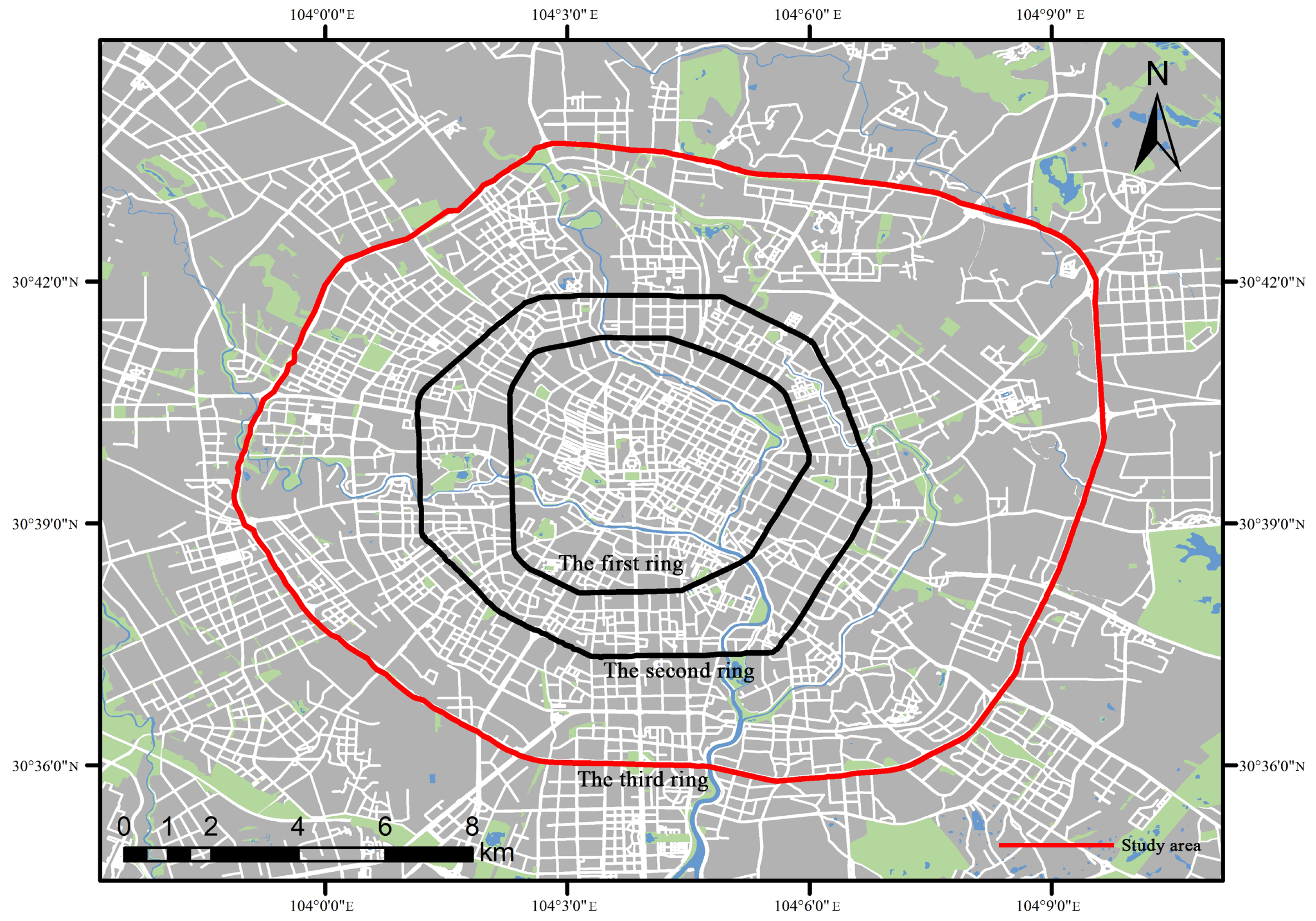
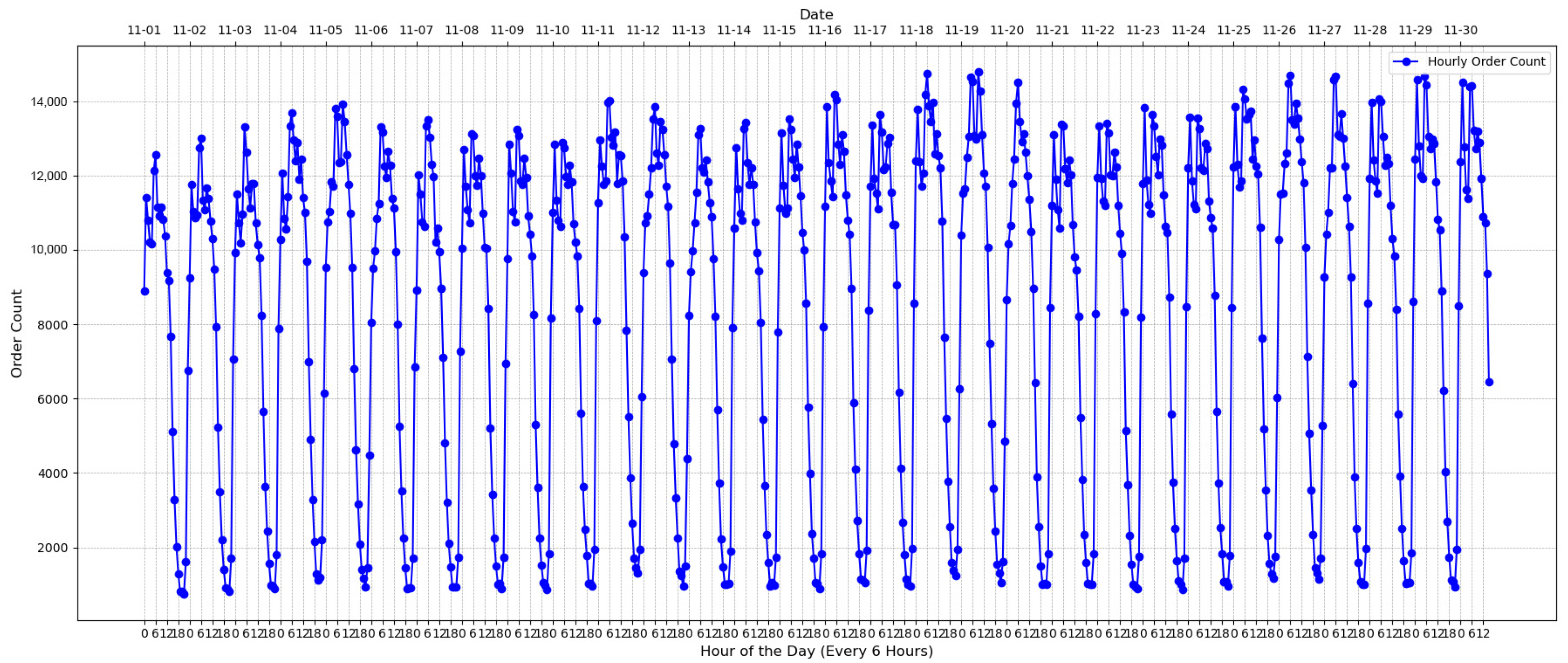
3.1. Data and Study Area
3.2. Dependent Variables
3.3. Independent Variables
3.3.1. “5D” Variables
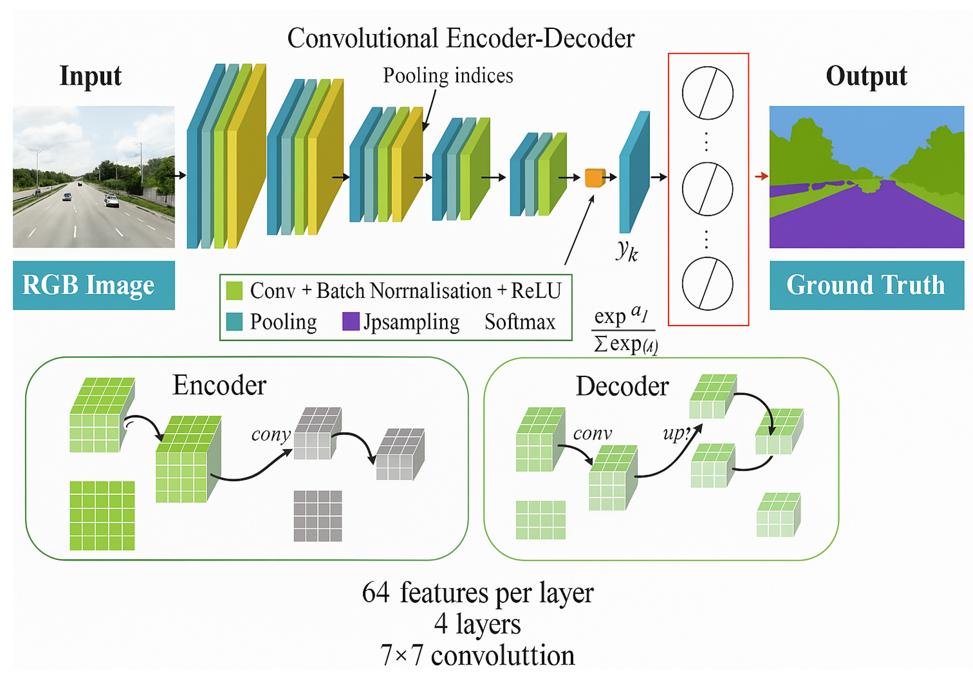
3.3.2. Visual Walkability Variables
3.4. Models
4. Results
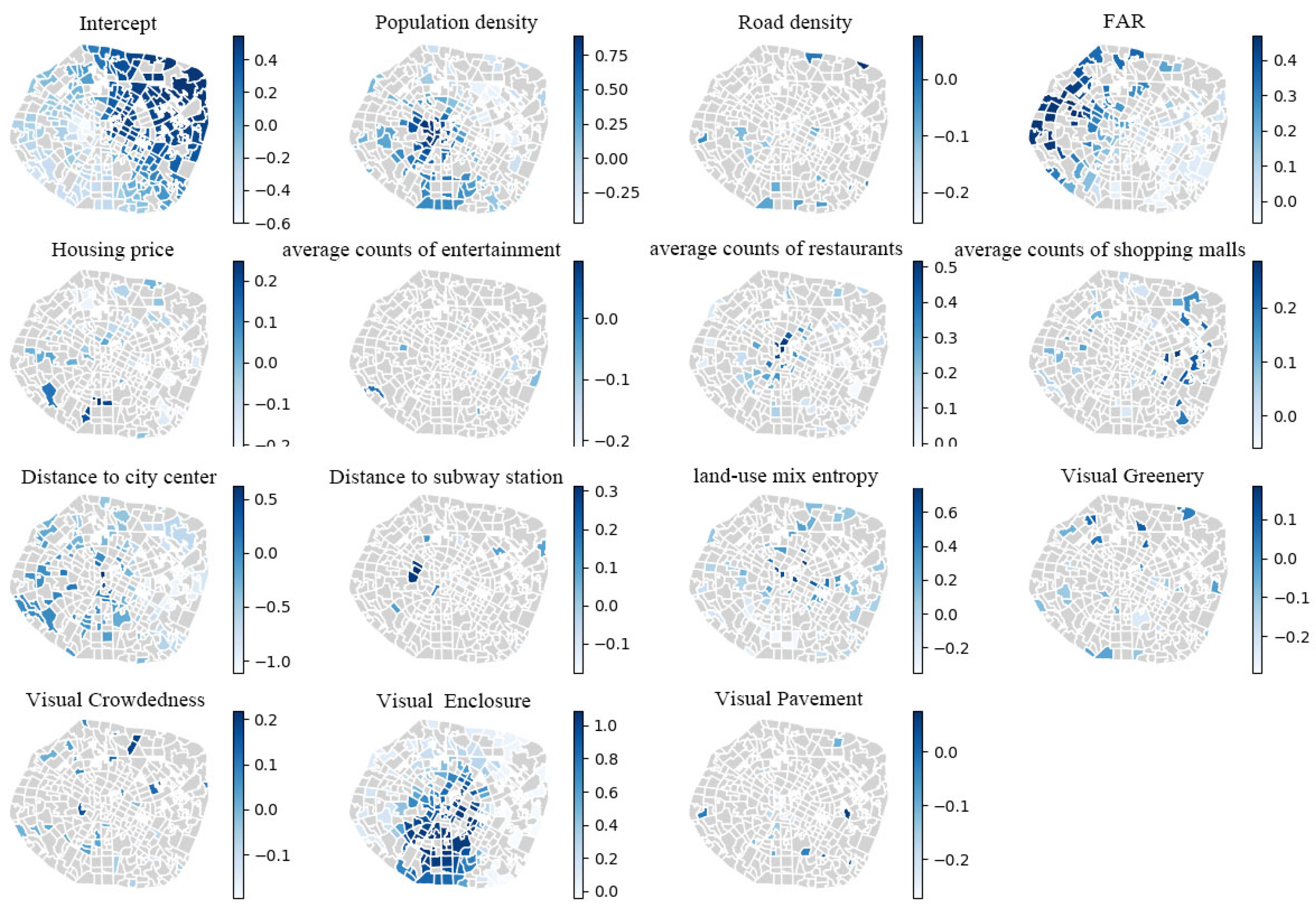
4.1. Morning Peak Hours Model
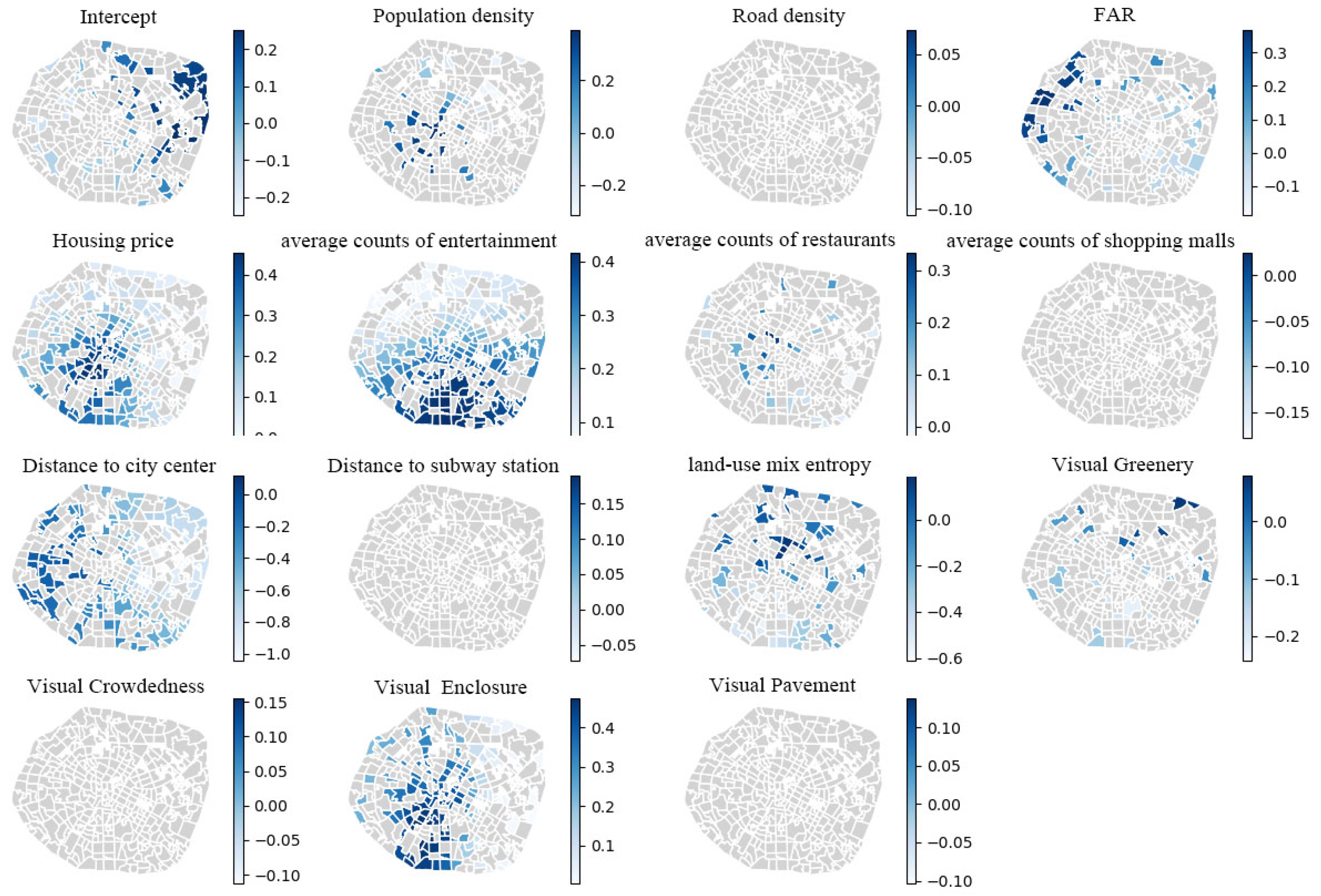
4.2. Evening Peak Hours Model
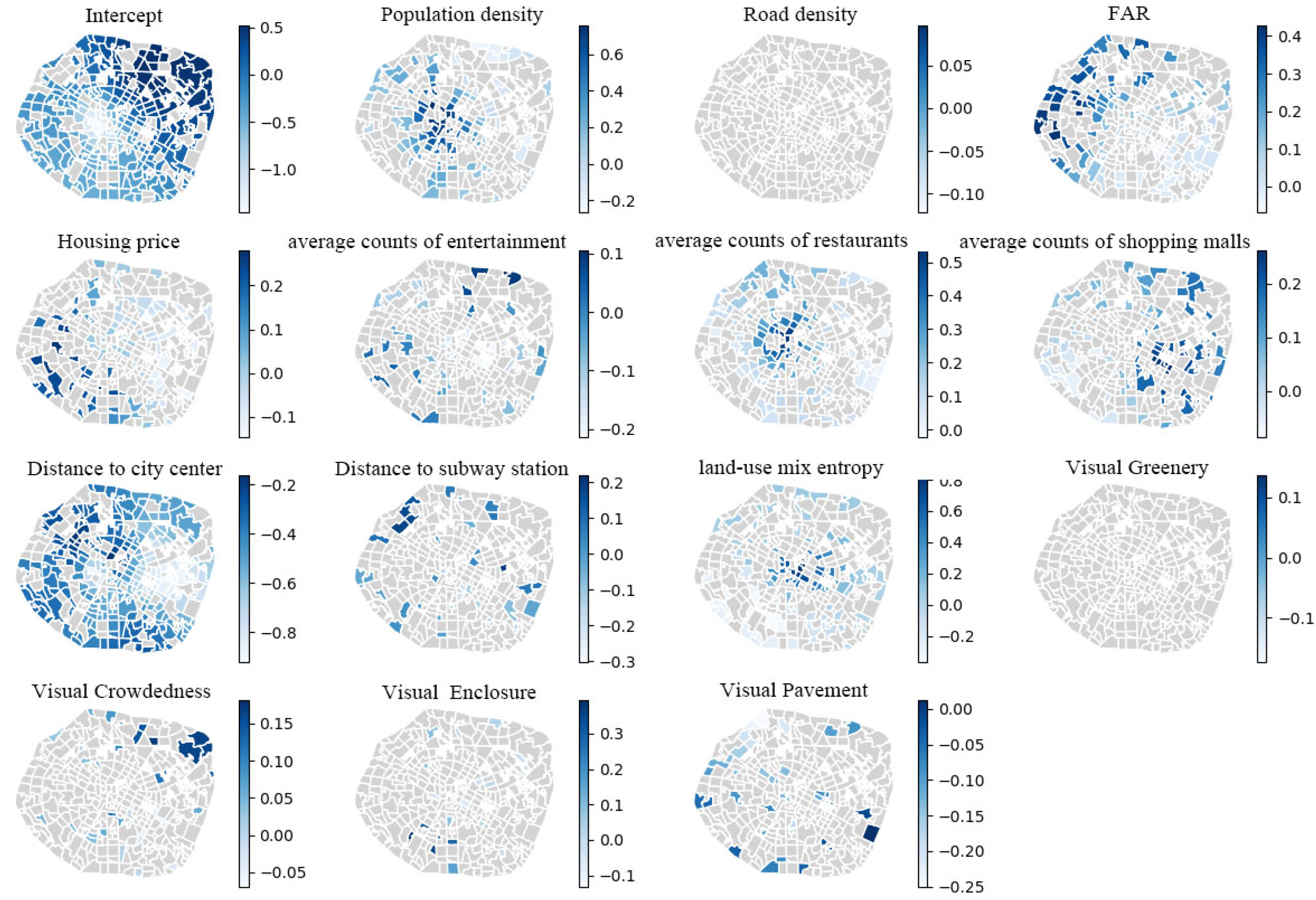
4.3. Nighttime Model
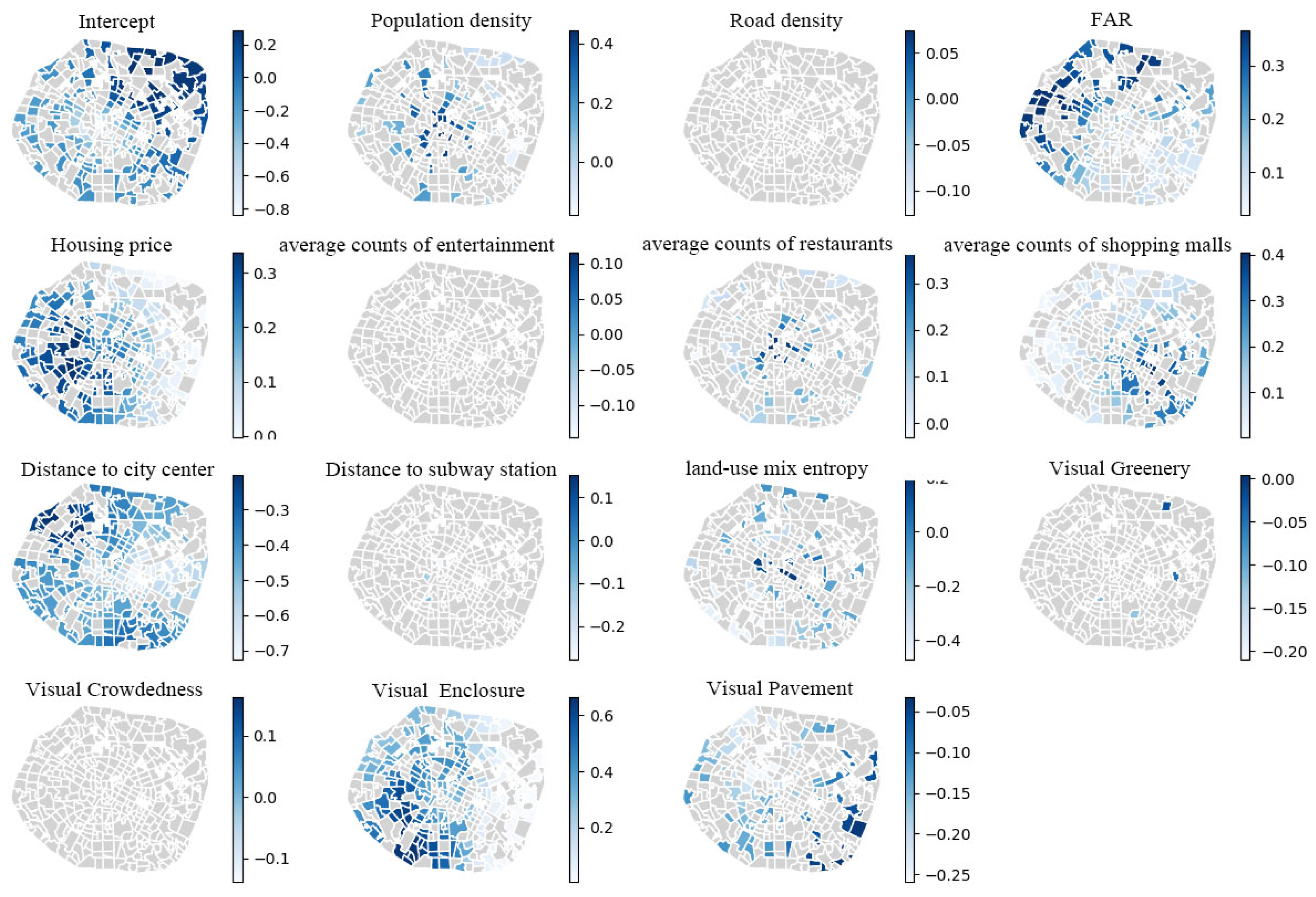
4.4. Casual Time Model
5. Discussion
5.1. OLS
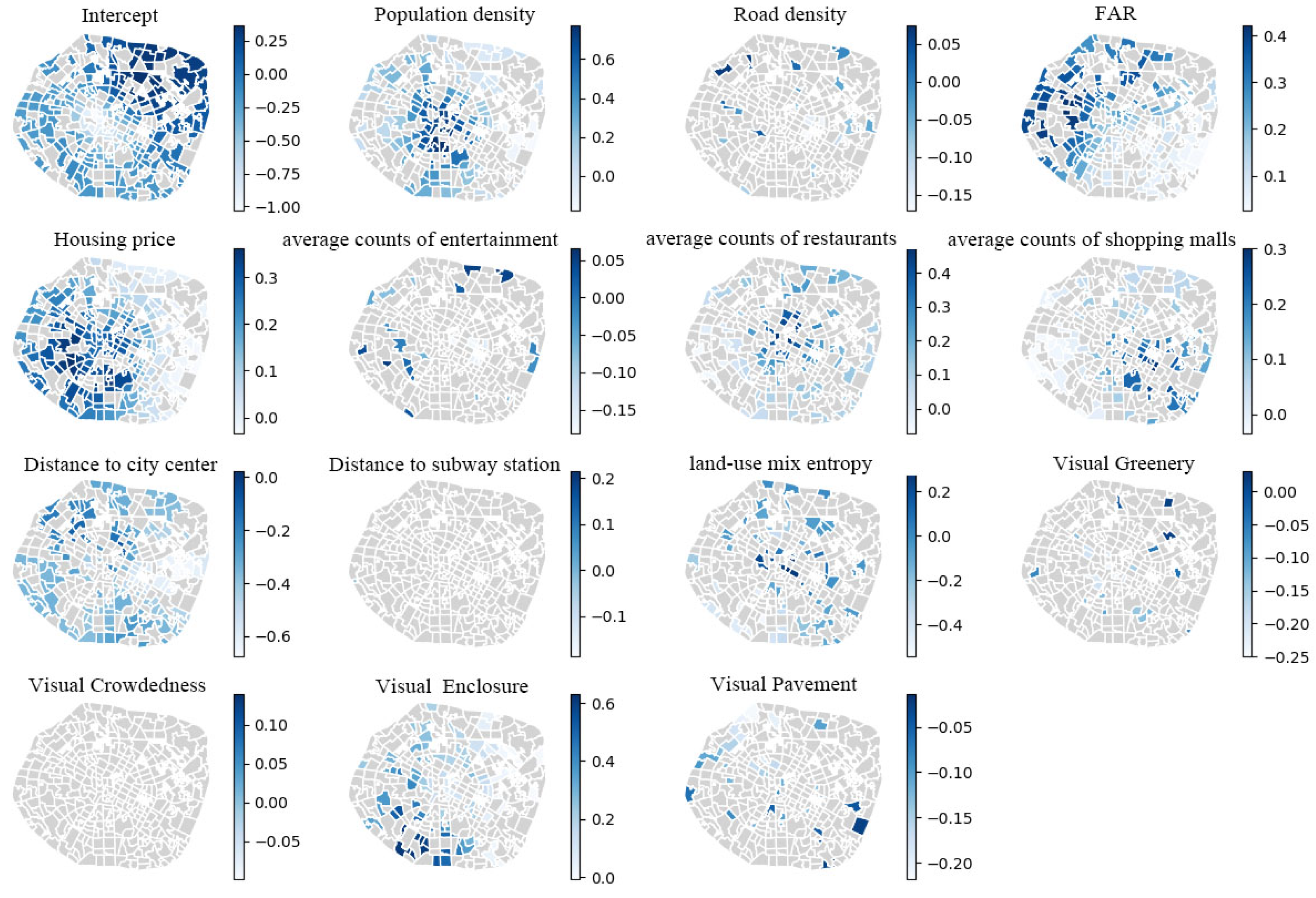
5.2. GWR
6. Conclusions
Author Contributions
Funding
Institutional Review Board Statement
Informed Consent Statement
Data Availability Statement
Conflicts of Interest
References
- DiDi. Didiglobal. Available online: https://www.didiglobal.com/ (accessed on 4 March 2025).
- Rayle, L.; Dai, D.; Chan, N.; Cervero, R.; Shaheen, S. Just a better taxi? A survey-based comparison of taxis, transit, and ridesourcing services in San Francisco. Transp. Policy 2016, 45, 168–178. [Google Scholar] [CrossRef]
- Yu, H.; Peng, Z.R. Exploring the spatial variation of ridesourcing demand and its relationship to built environment and socioeconomic factors with the geographically weighted Poisson regression. J. Transp. Geogr. 2019, 75, 147–163. [Google Scholar] [CrossRef]
- Shaheen, S.; Cohen, A.; Zohdy, I. Shared Mobility: Current Practices and Guiding Principles; Technical report; Federal Highway Administration: Washington, DC, USA, 2016.
- Wenzel, T.; Rames, C.; Kontou, E.; Henao, A. Travel and energy implications of ridesourcing service in Austin, Texas. Transp. Res. Part D Transp. Environ. 2019, 70, 18–34. [Google Scholar] [CrossRef]
- Alemi, F.; Circella, G.; Handy, S.; Mokhtarian, P. What influences travelers to use Uber? Exploring the factors affecting the adoption of on-demand ride services in California. Travel Behav. Soc. 2018, 13, 88–104. [Google Scholar] [CrossRef]
- Zhang, H.; Chen, J.; Li, W.; Song, X.; Shibasaki, R. Mobile phone GPS data in urban ride-sharing: An assessment method for emission reduction potential. Appl. Energy 2020, 269, 115038. [Google Scholar] [CrossRef]
- Jin, S.T.; Kong, H.; Wu, R.; Sui, D.Z. Ridesourcing, the sharing economy, and the future of cities. Cities 2018, 76, 96–104. [Google Scholar] [CrossRef]
- Lee, Y.; Chen, G.Y.H.; Circella, G.; Mokhtarian, P.L. Substitution or complementarity? A latent-class cluster analysis of ridehailing impacts on the use of other travel modes in three southern US cities. Transp. Res. Part D Transp. Environ. 2022, 104, 103167. [Google Scholar] [CrossRef]
- Ghaffar, A.; Mitra, S.; Hyland, M. Modeling determinants of ridesourcing usage: A census tract-level analysis of Chicago. Transp. Res. Part C Emerg. Technol. 2020, 119, 102769. [Google Scholar] [CrossRef]
- Ewing, R.; Cervero, R. Travel and the built environment: A meta-analysis. J. Am. Plan. Assoc. 2010, 76, 265–294. [Google Scholar] [CrossRef]
- Gössling, S. ICT and transport behavior: A conceptual review. Int. J. Sustain. Transp. 2018, 12, 153–164. [Google Scholar] [CrossRef]
- Doorley, R.; Pakrashi, V.; Ghosh, B. Quantifying the health impacts of active travel: Assessment of methodologies. Transp. Rev. 2015, 35, 559–582. [Google Scholar] [CrossRef]
- Frank, L.D.; Schmid, T.L.; Sallis, J.F.; Chapman, J.; Saelens, B.E. Linking objectively measured physical activity with objectively measured urban form: Findings from SMARTRAQ. Am. J. Prev. Med. 2005, 28, 117–125. [Google Scholar] [CrossRef] [PubMed]
- Jarrett, J.; Woodcock, J.; Griffiths, U.K.; Chalabi, Z.; Edwards, P.; Roberts, I.; Haines, A. Effect of increasing active travel in urban England and Wales on costs to the National Health Service. Lancet 2012, 379, 2198–2205. [Google Scholar] [CrossRef]
- Feigon, S.; Murphy, C. Shared Mobility and the Transformation of Public Transit; Number Project J-11, Task 21; American Public Transportation Association: Washington, DC, USA, 2016. [Google Scholar]
- Marquet, O. Spatial distribution of ride-hailing trip demand and its association with walkability and neighborhood characteristics. Cities 2020, 106, 102926. [Google Scholar] [CrossRef]
- Koo, B.W.; Guhathakurta, S.; Botchwey, N. How are neighborhood and street-level walkability factors associated with walking behaviors? A big data approach using street view images. Environ. Behav. 2022, 54, 211–241. [Google Scholar] [CrossRef]
- Wang, M.; Chen, Z.; Rong, H.H.; Mu, L.; Zhu, P.; Shi, Z. Ridesharing accessibility from the human eye: Spatial modeling of built environment with street-level images. Comput. Environ. Urban Syst. 2022, 97, 101858. [Google Scholar] [CrossRef]
- Brown, A. Redefining car access: Ride-hail travel and use in Los Angeles. J. Am. Plan. Assoc. 2019, 85, 83–95. [Google Scholar] [CrossRef]
- Cervero, R.; Kockelman, K. Travel demand and the 3Ds: Density, diversity, and design. Transp. Res. Part D Transp. Environ. 1997, 2, 199–219. [Google Scholar] [CrossRef]
- Clifton, K.J.; Currans, K.M.; Muhs, C.D. Adjusting ITE’s trip generation handbook for urban context. J. Transp. Land Use 2015, 8, 5–29. [Google Scholar] [CrossRef]
- Hooper, K.G. Trip Generation Handbook; Institute of Transportation Engineers: Washington, DC, USA, 2017.
- Stevens, M.R. Does compact development make people drive less? J. Am. Plan. Assoc. 2017, 83, 7–18. [Google Scholar] [CrossRef]
- Ewing, R.; Cervero, R. “Does compact development make people drive less?” The answer is yes. J. Am. Plan. Assoc. 2017, 83, 19–25. [Google Scholar] [CrossRef]
- Ewing, R.; Dumbaugh, E.; Brown, M. Internalizing travel by mixing land uses: Study of master-planned communities in South Florida. Transp. Res. Rec. 2001, 1780, 115–128. [Google Scholar] [CrossRef]
- Wu, C.; Ye, X.; Ren, F.; Du, Q. Check-in behaviour and spatio-temporal vibrancy: An exploratory analysis in Shenzhen, China. Cities 2018, 77, 104–116. [Google Scholar] [CrossRef]
- Ma, J.; Mitchell, G.; Heppenstall, A. Daily travel behaviour in Beijing, China: An analysis of workers’ trip chains, and the role of socio-demographics and urban form. Habitat Int. 2014, 43, 263–273. [Google Scholar] [CrossRef]
- Munshi, T. Built environment and mode choice relationship for commute travel in the city of Rajkot, India. Transp. Res. Part D Transp. Environ. 2016, 44, 239–253. [Google Scholar] [CrossRef]
- Sun, B.; Ermagun, A.; Dan, B. Built environmental impacts on commuting mode choice and distance: Evidence from Shanghai. Transp. Res. Part D Transp. Environ. 2017, 52, 441–453. [Google Scholar] [CrossRef]
- Buliung, R.N.; Larsen, K.; Faulkner, G.; Ross, T. Children’s independent mobility in the City of Toronto, Canada. Travel Behav. Soc. 2017, 9, 58–69. [Google Scholar] [CrossRef]
- Wang, Y.; Zheng, B.; Lim, E.P. Understanding the effects of taxi ride-sharing—A case study of Singapore. Comput. Environ. Urban Syst. 2018, 69, 124–132. [Google Scholar] [CrossRef]
- Zhang, B.; Chen, S.; Ma, Y.; Li, T.; Tang, K. Analysis on spatiotemporal urban mobility based on online car-hailing data. J. Transp. Geogr. 2020, 82, 102568. [Google Scholar] [CrossRef]
- Li, T.; Jing, P.; Li, L.; Sun, D.; Yan, W. Revealing the varying impact of urban built environment on online car-hailing travel in spatio-temporal dimension: An exploratory analysis in Chengdu, China. Sustainability 2019, 11, 1336. [Google Scholar] [CrossRef]
- Wang, S.; Noland, R.B. Variation in ride-hailing trips in Chengdu, China. Transp. Res. Part D Transp. Environ. 2021, 90, 102596. [Google Scholar] [CrossRef]
- Yuan, Y.; Raubal, M.; Liu, Y. Correlating mobile phone usage and travel behavior—A case study of Harbin, China. Comput. Environ. Urban Syst. 2012, 36, 118–130. [Google Scholar] [CrossRef]
- Chuang, I.T.; Beattie, L.; Feng, L. Analysing the relationship between proximity to transit stations and local living patterns: A study of human mobility within a 15 min walking distance through mobile location data. Urban Sci. 2023, 7, 105. [Google Scholar] [CrossRef]
- Wang, D.; Cao, X. Impacts of the built environment on activity-travel behavior: Are there differences between public and private housing residents in Hong Kong? Transp. Res. Part A Policy Pract. 2017, 103, 25–35. [Google Scholar] [CrossRef]
- Lozano Landinez, F.; Shastry, S. Hailed or Ride-Sourced? A Descriptive Study of Four Indian Cities. In Proceedings of the Transportation Research Board 97th Annual Meeting, Washington, DC, USA, 7–11 January 2018. [Google Scholar]
- Zheng, Z.; Zhang, J.; Zhang, L.; Li, M.; Rong, P.; Qin, Y. Understanding the impact of the built environment on ride-hailing from a spatio-temporal perspective: A fine-scale empirical study from China. Cities 2022, 126, 103706. [Google Scholar] [CrossRef]
- Li, B.; Cai, Z.; Jiang, L.; Su, S.; Huang, X. Exploring urban taxi ridership and local associated factors using GPS data and geographically weighted regression. Cities 2019, 87, 68–86. [Google Scholar] [CrossRef]
- Zhang, W.; Ukkusuri, S.V.; Lu, J.J. Impacts of urban built environment on empty taxi trips using limited geolocation data. Transportation 2017, 44, 1445–1473. [Google Scholar] [CrossRef]
- Zhu, P.; Huang, J.; Wang, J.; Liu, Y.; Li, J.; Wang, M.; Qiang, W. Understanding taxi ridership with spatial spillover effects and temporal dynamics. Cities 2022, 125, 103637. [Google Scholar] [CrossRef]
- National Academies of Sciences, Engineering, and Medicine (U.S.). Between Public and Private Mobility: Examining the Rise of Technology-Enabled Transportation Services; Transportation Research Board: Washington, DC, USA, 2016. [Google Scholar]
- Neves, A.; Brand, C. Assessing the potential for carbon emissions savings from replacing short car trips with walking and cycling using a mixed GPS-travel diary approach. Transp. Res. Part A Policy Pract. 2019, 123, 130–146. [Google Scholar] [CrossRef]
- Grabow, M.L.; Bernardinello, M.; Bersch, A.J.; Engelman, C.D.; Martinez-Donate, A.; Patz, J.A.; Peppard, P.E.; Malecki, K.M. What moves us: Subjective and objective predictors of active transportation. J. Transp. Health 2019, 15, 100625. [Google Scholar] [CrossRef]
- Buehler, R.; Götschi, T.; Winters, M. Moving Toward Active Transportation: How Policies Can Encourage Walking and Bicycling; Active Living Research: San Diego, CA, USA, 2016. [Google Scholar]
- Zhou, H.; He, S.; Cai, Y.; Wang, M.; Su, S. Social inequalities in neighborhood visual walkability: Using street view imagery and deep learning technologies to facilitate healthy city planning. Sustain. Cities Soc. 2019, 50, 101605. [Google Scholar] [CrossRef]
- Moura, F.; Cambra, P.; Gonçalves, A.B. Measuring walkability for distinct pedestrian groups with a participatory assessment method: A case study in Lisbon. Landsc. Urban Plan. 2017, 157, 282–296. [Google Scholar] [CrossRef]
- Taleai, M.; Amiri, E.T. Spatial multi-criteria and multi-scale evaluation of walkability potential at street segment level: A case study of Tehran. Sustain. Cities Soc. 2017, 31, 37–50. [Google Scholar] [CrossRef]
- Adams, M.A.; Ryan, S.; Kerr, J.; Sallis, J.F.; Patrick, K.; Frank, L.D.; Norman, G.J. Validation of the Neighborhood Environment Walkability Scale (NEWS) items using geographic information systems. J. Phys. Act. Health 2009, 6, S113–S123. [Google Scholar] [CrossRef]
- Cerin, E.; Saelens, B.E.; Sallis, J.F.; Frank, L.D. Neighborhood Environment Walkability Scale: Validity and development of a short form. Med. Sci. Sport. Exerc. 2006, 38, 1682. [Google Scholar] [CrossRef] [PubMed]
- Moniruzzaman, M.; Páez, A. A model-based approach to select case sites for walkability audits. Health Place 2012, 18, 1323–1334. [Google Scholar] [CrossRef]
- Naik, N.; Philipoom, J.; Raskar, R.; Hidalgo, C. Streetscore-predicting the perceived safety of one million streetscapes. In Proceedings of the IEEE Conference on Computer Vision and Pattern Recognition Workshops, Columbus, OH, USA, 23–28 June 2014; pp. 779–785. [Google Scholar]
- Hu, L.; He, S.; Han, Z.; Xiao, H.; Su, S.; Weng, M.; Cai, Z. Monitoring housing rental prices based on social media: An integrated approach of machine-learning algorithms and hedonic modeling to inform equitable housing policies. Land Use Policy 2019, 82, 657–673. [Google Scholar] [CrossRef]
- Lu, Y.; Sarkar, C.; Xiao, Y. The effect of street-level greenery on walking behavior: Evidence from Hong Kong. Soc. Sci. Med. 2018, 208, 41–49. [Google Scholar] [CrossRef]
- Yin, L.; Wang, Z. Measuring visual enclosure for street walkability: Using machine learning algorithms and Google Street View imagery. Appl. Geogr. 2016, 76, 147–153. [Google Scholar] [CrossRef]
- Zeng, L.; Lu, J.; Li, W.; Li, Y. A fast approach for large-scale Sky View Factor estimation using street view images. Build. Environ. 2018, 135, 74–84. [Google Scholar] [CrossRef]
- Li, X.; Ratti, C. Mapping the spatial distribution of shade provision of street trees in Boston using Google Street View panoramas. Urban For. Urban Green. 2018, 31, 109–119. [Google Scholar] [CrossRef]
- Richards, D.R.; Edwards, P.J. Quantifying street tree regulating ecosystem services using Google Street View. Ecol. Indic. 2017, 77, 31–40. [Google Scholar] [CrossRef]
- DiDi. CBNData. Available online: https://cbndata.com/report/112?isReading=report&page=4 (accessed on 4 March 2025).
- Qiao, S.; Yeh, A.G.O. Is ride-hailing a valuable means of transport in newly developed areas under TOD-oriented urbanization in China? Evidence from Chengdu City. J. Transp. Geogr. 2021, 96, 103183. [Google Scholar] [CrossRef]
- Pezzulo, C.; Hornby, G.M.; Sorichetta, A.; Gaughan, A.E.; Linard, C.; Bird, T.J.; Kerr, D.; Lloyd, C.T.; Tatem, A.J. Sub-national mapping of population pyramids and dependency ratios in Africa and Asia. Sci. Data 2017, 4, 170089. [Google Scholar] [CrossRef]
- Zhang, C.; Jia, S.; Yang, R. Housing affordability and housing vacancy in China: The role of income inequality. J. Hous. Econ. 2016, 33, 4–14. [Google Scholar] [CrossRef]
- Song, Y.; Merlin, L.; Rodriguez, D. Comparing measures of urban land use mix. Comput. Environ. Urban Syst. 2013, 42, 1–13. [Google Scholar] [CrossRef]
- Wang, K.; Zhang, C.; Li, W. Comparison of geographically weighted regression and regression kriging for estimating the spatial distribution of soil organic matter. Gisci. Remote Sens. 2012, 49, 915–932. [Google Scholar] [CrossRef]
- Lewis, S. Neighborhood density and travel mode: New survey findings for high densities. Int. J. Sustain. Dev. World Ecol. 2018, 25, 152–165. [Google Scholar] [CrossRef]
- Lu, Y.; Sun, G.; Sarkar, C.; Gou, Z.; Xiao, Y. Commuting mode choice in a high-density city: Do land-use density and diversity matter in Hong Kong? Int. J. Environ. Res. Public Health 2018, 15, 920. [Google Scholar] [CrossRef]
- Wang, Z.; Gong, X.; Zhang, Y.; Liu, S.; Chen, N. Multi-scale geographically weighted elasticity regression model to explore the elastic effects of the built environment on ride-hailing ridership. Sustainability 2023, 15, 4966. [Google Scholar] [CrossRef]
- Clewlow, R.R.; Mishra, G.S. Disruptive Transportation: The Adoption, Utilization, and Impacts of Ride-Hailing in the United States; University of California: Berkeley, CA, USA, 2017. [Google Scholar]
- Lai, J.; Wang, Y.; Yang, Y.; Wu, X.; Zhang, Y. Exploring the built environment impacts on Online Car-hailing waiting time: An empirical study in Beijing. Comput. Environ. Urban Syst. 2025, 115, 102205. [Google Scholar] [CrossRef]
- Henao, A.; Marshall, W.E. The impact of ride-hailing on vehicle miles traveled. Transportation 2019, 46, 2173–2194. [Google Scholar] [CrossRef]
- Yin, J.; Zhao, F.; Tang, W.; Ma, J. The Nonlinear and Threshold Effect of Built Environment on Ride-Hailing Travel Demand. Appl. Sci. 2024, 14, 4072. [Google Scholar] [CrossRef]
- Zhao, F.; Ma, J.; Yin, C.; Tang, W.; Wang, X.; Yin, J. Spatiotemporal Heterogeneous Effects of Built Environment and Taxi Demand on Ride-Hailing Ridership. Appl. Sci. 2024, 14, 142. [Google Scholar] [CrossRef]
- Wu, J.; Wang, B.; Ta, N.; Zhou, K.; Chai, Y. Does street greenery always promote active travel? Evidence from Beijing. Urban For. Urban Green. 2020, 56, 126886. [Google Scholar] [CrossRef]
- Yang, L.; Yang, H.; Yu, B.; Lu, Y.; Cui, J.; Lin, D. Exploring non-linear and synergistic effects of green spaces on active travel using crowdsourced data and interpretable machine learning. Travel Behav. Soc. 2024, 34, 100673. [Google Scholar] [CrossRef]
- Yu, J.; Zhang, H.; Dong, X.; Shen, J. The impact of street greenery on active travel: A narrative systematic review. Front. Public Health 2024, 12, 1337804. [Google Scholar] [CrossRef]
- Song, J.; Zhou, S.; Kwan, M.P.; Liang, S.; Lu, J.; Jing, F.; Wang, L. The effect of eye-level street greenness exposure on walking satisfaction: The mediating role of noise and PM2. 5. Urban For. Urban Green. 2022, 77, 127752. [Google Scholar] [CrossRef]
- RichBLambert. How to Create Walking Friendly Cities. Available online: https://naturalwalkingcities.com/how-to-make-cities-walking-friendly/ (accessed on 4 March 2025).
- Li, X.; Xu, J.; Du, M.; Liu, D.; Kwan, M.P. Understanding the spatiotemporal variation of ride-hailing orders under different travel distances. Travel Behav. Soc. 2023, 32, 100581. [Google Scholar] [CrossRef]
- Du, M.; Li, X.; Kwan, M.P.; Yang, J.; Liu, Q. Understanding the spatiotemporal variation of high-efficiency ride-hailing orders: A case study of Haikou, China. ISPRS Int. J. Geo-Inf. 2022, 11, 42. [Google Scholar] [CrossRef]
- Ki, D.; Lee, S. Analyzing the effects of Green View Index of neighborhood streets on walking time using Google Street View and deep learning. Landsc. Urban Plan. 2021, 205, 103920. [Google Scholar] [CrossRef]
- Liu, B.; Ji, Y.; Cats, O. Integrating ride-hailing services with public transport: A stochastic user equilibrium model for multimodal transport systems. Transp. A Transp. Sci. 2025, 21, 2236240. [Google Scholar] [CrossRef] [PubMed]


| Indicators | Definition | Formula |
|---|---|---|
| Visual Greenery | Visual Greenery is the street vegetation that pedestrians can see. | Visual greenery = |
| Visual Crowdedness | Visual Crowdedness measures spatial oppression through the proportion of buildings and motor vehicles. | Visual crowdedness = |
| Visual Enclosure | Visual Enclosure assesses visual openness through sky openness and interface permeability, which means the ratio of vertical objects to horizontal features. | Visual enclosure = |
| Visual Pavement | Visual Pavement determines pedestrian safety through sidewalk proportion. | Visual pavement = |
| Min | Max | Mean | Std. Dev. | ||
|---|---|---|---|---|---|
| Trips in morning peak hours/community area | average pick-ups (sum = 1,678,964) | 92.12 | 37,627 | 4866.56 | 6100.813 |
| average drop-offs (sum = 1,598,715) | 38.34 | 40,956 | 4633.96 | 5314.522 | |
| Trips in afternoon peak hours/community area | average pick-ups (sum = 263,961.3) | 0 | 6047.9 | 765.1 | 1005.995 |
| average drop-offs (sum = 227,851.3) | 0 | 5522.4 | 660.4 | 638.7626 | |
| Trips in night hours/community area | average pick-ups (sum = 3,329,599) | 69.38 | 46,844 | 9651.01 | 9152.022 |
| average drop-offs (sum = 3,617,335) | 41.83 | 103,365 | 10,485.03 | 14,742.28 | |
| Trips in recreation hours/community area | average pick-ups (sum = 1,545,129) | 45.8 | 31,870 | 4478.6 | 4669.945 |
| average drop-offs (sum = 1,527,366) | 43.22 | 37,686 | 4427.15 | 5093.238 | |
| Population density (residents/km2) | 3996.2 | 62,731 | 25,476.24 | 8786.411 | |
| Road density (km/km2) | 0 | 37.181 | 9.652022 | 4.984533 | |
| FAR | 0 | 13.462 | 2.625983 | 1.617472 | |
| Housing price by cell (CNY/m2) | 0 | 43,105 | 15,863.12 | 6071.479 | |
| Average counts of entertainments | 0 | 268.53 | 36.26 | 34.61367 | |
| Average counts of restaurants | 0 | 739.23 | 160.97 | 129.4699 | |
| Average counts of shopping malls | 0 | 90.921 | 11.168 | 9.458874 | |
| Distance to city center (m) | 220 | 9686 | 4740 | 2053.016 | |
| Distance to subway station (m) | 74.89 | 3279.6 | 759.03 | 532.7586 | |
| Land-use mix entropy | 2 × 10 −7 | 0.9872 | 0.828126 | 0.145013 | |
| Visual Greenery | 0.0607 | 0.5333 | 0.22761 | 0.076622 | |
| Visual Crowdedness | 0.0108 | 0.1343 | 0.05492 | 0.015487 | |
| Visual Enclosure | 0.7052 | 176.45 | 5.1521 | 13.14099 | |
| Visual Pavement | 0.024 | 0.5809 | 0.27674 | 0.096921 |
| GWR | OLS | ||||
|---|---|---|---|---|---|
| Variables | Min | Median | Max | St. Dev. | Coef. |
| Intercept | −1.033 | −0.155 | 0.367 | 0.278 | −1.8 × 10⁻¹⁶ |
| Population density | −0.18 | 0.219 | 0.773 | 0.247 | 0.1913 ** |
| Road density | −0.172 | −0.059 | 0.074 | 0.061 | −0.07469 . |
| FAR | 0.025 | 0.224 | 0.422 | 0.123 | 0.2949 *** |
| Average housing price | −0.035 | 0.217 | 0.362 | 0.117 | 0.1462 *** |
| Average counts of entertainment | −0.182 | −0.059 | 0.066 | 0.064 | −0.05239 |
| Average counts of restaurants | −0.075 | 0.162 | 0.474 | 0.12 | 0.116 . |
| Average counts of shopping malls | −0.036 | 0.096 | 0.301 | 0.092 | 0.1397 ** |
| Distance to city center | −0.676 | −0.349 | 0.023 | 0.134 | −0.314 *** |
| Distance to subway station | −0.188 | 0.025 | 0.215 | 0.087 | 0.04355 |
| Land-use mix entropy | −0.543 | −0.056 | 0.292 | 0.191 | −0.2085 *** |
| Visual Greenery | −0.25 | −0.093 | 0.032 | 0.063 | −0.0947 * |
| Visual Crowdedness | −0.099 | 0.042 | 0.14 | 0.062 | 0.03279 |
| Visual Enclosure | −0.006 | 0.215 | 0.632 | 0.166 | 0.1051 ** |
| Visual Pavement | −0.218 | −0.11 | −0.013 | 0.05 | −0.147 ** |
| Adj.R2 | 0.753 | 0.629 | |||
| AICc | −17,654.541 | −12,670.456 | |||
| Moran’s I | 0.431 *** | ||||
| Bandwidth | 162 | ||||
| GWR | OLS | ||||
|---|---|---|---|---|---|
| Variables | Min | Median | Max | St. Dev. | Coef. |
| Intercept | −0.646 | −0.096 | 0.353 | 0.231 | −3.1 × 10⁻¹⁶ |
| Population density | −0.151 | 0.165 | 0.481 | 0.173 | 0.145 . |
| Road density | −0.185 | −0.055 | 0.042 | 0.054 | −0.06795 |
| FAR | −0.047 | 0.129 | 0.365 | 0.131 | 0.2096 ** |
| Average housing price | −0.019 | 0.258 | 0.495 | 0.147 | 0.1597 *** |
| Average counts of entertainment | −0.207 | −0.089 | 0.135 | 0.075 | −0.06291 |
| Average counts of restaurants | 0.038 | 0.233 | 0.573 | 0.12 | 0.2091 ** |
| Average counts of shopping malls | −0.015 | 0.09 | 0.266 | 0.081 | 0.0954 . |
| Distance to city center | −0.74 | −0.355 | 0.157 | 0.196 | −0.3309 *** |
| Distance to subway station | −0.151 | 0.04 | 0.236 | 0.079 | 0.05926 |
| Land-use mix entropy | −0.553 | −0.036 | 0.258 | 0.203 | −0.1646 ** |
| Visual Greenery | −0.3 | −0.108 | 0.034 | 0.083 | −0.09361 * |
| Visual Crowdedness | −0.151 | 0.026 | 0.12 | 0.075 | 0.01884 |
| Visual Enclosure | −0.064 | 0.107 | 0.39 | 0.114 | 0.08026 * |
| Visual Pavement | −0.198 | −0.07 | 0.046 | 0.058 | −0.1234 * |
| Adj.R2 | 0.623 | 0.521 | |||
| AICc | −23,901.615 | −18,456.219 | |||
| Moran’s I | 0.528 *** | ||||
| Bandwidth | 185 | ||||
| GWR | OLS | ||||
|---|---|---|---|---|---|
| Variables | Min | Median | Max | St. Dev. | Coef. |
| Intercept | −0.25 | 0.03 | 0.251 | 0.134 | 2.162 × 10⁻¹⁶ |
| Population density | −0.316 | 0.066 | 0.39 | 0.213 | 0.06701 |
| Road density | −0.107 | −0.032 | 0.073 | 0.042 | −0.03154 |
| FAR | −0.188 | 0.074 | 0.367 | 0.15 | 0.1147 |
| Average housing price | −0.002 | 0.198 | 0.454 | 0.127 | 0.1425 ** |
| Average counts of entertainment | 0.069 | 0.255 | 0.417 | 0.111 | 0.2781 *** |
| Average counts of restaurants | −0.022 | 0.13 | 0.334 | 0.094 | 0.1157 |
| Average counts of retails | −0.179 | −0.083 | 0.025 | 0.062 | −0.06012 |
| Distance to city center | −1.044 | −0.401 | 0.119 | 0.287 | −0.3371 ** |
| Distance to subway station | −0.073 | 0.082 | 0.19 | 0.047 | 0.06258 |
| Land-use mix entropy | −0.612 | −0.133 | 0.191 | 0.208 | −0.159 ** |
| Visual Greenery | −0.243 | −0.088 | 0.08 | 0.083 | −0.0696 |
| Visual Crowdedness | −0.113 | 0.035 | 0.156 | 0.076 | 0.0348 |
| Visual Enclosure | 0.004 | 0.25 | 0.474 | 0.149 | 0.08475 * |
| Visual Pavement | −0.104 | 0.017 | 0.139 | 0.062 | −0.02996 |
| Adj.R2 | 0.721 | 0.674 | |||
| AICc | −16,549.231 | −14,320.636 | |||
| Moran’s I | 0.396 *** | ||||
| Bandwidth | 207 | ||||
| GWR | OLS | ||||
|---|---|---|---|---|---|
| Variables | Min | Median | Max | St. Dev. | Coef. |
| Intercept | −0.602 | 0.078 | 0.546 | 375 | 1.021 × 10⁻¹⁷ |
| Population density | −0.475 | 0.172 | 0.89 | 0.005839 | 0.226 ** |
| Road density | −0.255 | −0.061 | 0.076 | 5.787 | −0.09337 * |
| FAR | −0.062 | 0.141 | 0.469 | 28.14 | 0.1828 * |
| Average housing price | −0.208 | −0.061 | 0.248 | 0.00503 | −0.03487 |
| Average counts of entertainment | −0.213 | −0.056 | 0.094 | 1.123 | −0.06585 |
| Average counts of restaurants | −0.014 | 0.129 | 0.517 | 0.3525 | 0.148 * |
| Average counts of retails | −0.06 | 0.078 | 0.287 | 3.681 | 0.2035 *** |
| Distance to city center | −1.114 | −0.253 | 0.623 | 0.03124 | −0.2222 * |
| Distance to subway station | −0.178 | 0.042 | 0.314 | 0.05676 | 0.03738 |
| Land-use mix entropy | −0.35 | 0.11 | 0.756 | 254.8 | −0.03498 |
| Visual Greenery | −0.294 | −0.066 | 0.187 | 388.5 | −0.07183 |
| Visual Crowdedness | −0.196 | 0.037 | 0.219 | 1785 | 0.04493 |
| Visual Enclosure | −0.041 | 0.314 | 1.089 | 2.025 | 0.08798 * |
| Visual Pavement | −0.273 | −0.074 | 0.077 | 337.9 | −0.1368 ** |
| Adj.R2 | 0.751 | 0.722 | |||
| AICc | −14,503.853 | −11,923.350 | |||
| Moran’s I | 0.568 *** | ||||
| Bandwidth | 149 | ||||
| GWR | OLS | ||||
|---|---|---|---|---|---|
| Variables | Min | Median | Max | St. Dev. | Coef. |
| Intercept | −1.464 | −0.181 | 0.52 | 0.41 | 1.68 × 10⁻¹⁷ |
| Population density | −0.268 | 0.144 | 0.757 | 0.243 | 0.2091 ** |
| Road density | −0.123 | −0.017 | 0.097 | 0.054 | −0.07127 . |
| FAR | −0.07 | 0.132 | 0.428 | 0.149 | 0.2224 *** |
| Average housing price | −0.147 | 0.02 | 0.281 | 0.122 | 0.02056 |
| Avg. counts of entertainment | −0.214 | −0.067 | 0.105 | 0.077 | −0.1045 * |
| Avg. counts of restaurants | −0.024 | 0.152 | 0.536 | 0.123 | 0.1407 * |
| Avg. counts of retails | −0.087 | 0.094 | 0.263 | 0.088 | 0.1232 * |
| Distance to city center | −0.921 | −0.43 | −0.161 | 0.173 | −0.3955 *** |
| Distance to subway station | −0.303 | 0.013 | 0.22 | 0.114 | 0.06498 |
| Land-use mix entropy | −0.367 | 0.06 | 0.831 | 0.273 | −0.08533 . |
| Visual Greenery | −0.175 | −0.053 | 0.138 | 0.072 | −0.07819 . |
| Visual Crowdedness | −0.07 | 0.048 | 0.182 | 0.059 | 0.04743 |
| Visual Enclosure | −0.133 | 0.026 | 0.396 | 0.144 | 0.04817 |
| Visual Pavement | −0.251 | −0.091 | 0.013 | 0.062 | −0.1703 *** |
| Adj.R2 | 0.875 | 0.811 | |||
| AICc | −24,011.650 | −21,789.121 | |||
| Moran’s I | 0.620 *** | ||||
| Bandwidth | 145 | ||||
| GWR | OLS | ||||
|---|---|---|---|---|---|
| Variables | Min | Median | Max | St. Dev. | Coef. |
| Intercept | −0.842 | −0.127 | 0.285 | 0.228 | −2 × 10⁻¹⁷ |
| Population density | −0.183 | 0.143 | 0.445 | 0.158 | 0.1007 |
| Road density | −0.127 | −0.04 | 0.074 | 0.044 | −0.05766 |
| FAR | 0.019 | 0.188 | 0.366 | 0.109 | 0.2694 *** |
| Average housing price | −0.003 | 0.198 | 0.337 | 0.1 | 0.1416 ** |
| Avg. counts of entertainment | −0.146 | −0.054 | 0.116 | 0.063 | −0.03186 |
| Avg. counts of restaurants | −0.031 | 0.124 | 0.366 | 0.088 | 0.09014 |
| Avg. counts of retails | 0.002 | 0.148 | 0.404 | 0.11 | 0.1861 *** |
| Distance to city center | −0.727 | −0.427 | −0.2 | 0.119 | −0.3775 *** |
| Distance to subway station | −0.279 | −0.03 | 0.154 | 0.088 | 0.01201 |
| Land-use mix entropy | −0.473 | −0.113 | 0.21 | 0.161 | −0.2254 *** |
| Visual Greenery | −0.21 | −0.089 | 0.005 | 0.041 | −0.08202 . |
| Visual Crowdedness | −0.138 | 0.012 | 0.163 | 0.081 | 0.01187 |
| Visual Enclosure | 0.007 | 0.341 | 0.665 | 0.185 | 0.1186 ** |
| Visual Pavement | −0.259 | −0.146 | −0.032 | 0.061 | −0.1673 *** |
| Adj.R2 | 0.710 | 0.682 | |||
| AICc | −22,067.144 | −20,137.250 | |||
| Moran’s I | 0.597 *** | ||||
| Bandwidth | 149 | ||||
| GWR | OLS | ||||
|---|---|---|---|---|---|
| Variables | Min | Median | Max | St. Dev. | Coef. |
| Intercept | −0.652 | −0.091 | 0.486 | 0.279 | 1.83 × 10⁻¹⁶ |
| Population density | −0.148 | 0.231 | 0.665 | 0.219 | 0.2136 ** |
| Road density | −0.227 | −0.085 | 0.061 | 0.074 | −0.0884 * |
| FAR | 0.019 | 0.194 | 0.439 | 0.133 | 0.246 *** |
| Average housing price | −0.059 | 0.187 | 0.458 | 0.140 | 0.105 * |
| Avg. counts of entertainment | −0.201 | −0.073 | 0.111 | 0.075 | −0.05974 |
| Avg. counts of restaurants | −0.020 | 0.215 | 0.556 | 0.127 | 0.1822 ** |
| Avg. counts of retails | −0.047 | 0.060 | 0.197 | 0.062 | 0.08243 |
| Distance to city center | −0.724 | −0.249 | 0.575 | 0.241 | −0.2689 ** |
| Distance to subway station | −0.092 | 0.078 | 0.279 | 0.085 | 0.07149 |
| Land-use mix entropy | −0.520 | 0.020 | 0.355 | 0.222 | −0.128 * |
| Visual Greenery | −0.290 | −0.128 | 0.021 | 0.079 | −0.1165 ** |
| Visual Crowdedness | −0.123 | 0.040 | 0.124 | 0.064 | 0.03445 |
| Visual Enclosure | −0.012 | 0.109 | 0.458 | 0.135 | 0.06823 . |
| Visual Pavement | −0.185 | −0.064 | 0.057 | 0.054 | −0.1186 * |
| Adj.R2 | 0.742 | 0.711 | |||
| AICc | −21,003.167 | −19,082.249 | |||
| Moran’s I | 0.467 *** | ||||
| Bandwidth | 181 | ||||
| GWR | OLS | ||||
|---|---|---|---|---|---|
| Variables | Min | Median | Max | St. Dev. | Coef. |
| Intercept | −0.592 | −0.076 | 0.421 | 0.240 | 2.91 × 10⁻¹⁶ |
| Population density | −0.158 | 0.145 | 0.377 | 0.145 | 0.1306 . |
| Road density | −0.193 | −0.079 | 0.050 | 0.060 | −0.08376 . |
| FAR | 0.043 | 0.205 | 0.390 | 0.112 | 0.2517 *** |
| Average housing price | −0.028 | 0.219 | 0.435 | 0.137 | 0.1228 ** |
| Avg. counts of entertainment | −0.199 | −0.097 | 0.130 | 0.073 | −0.07013 |
| Avg. counts of restaurants | 0.026 | 0.203 | 0.476 | 0.101 | 0.1758 * |
| Avg. counts of retails | 0.016 | 0.128 | 0.284 | 0.071 | 0.1387 ** |
| Distance to city center | −0.689 | −0.320 | 0.239 | 0.185 | −0.310 ** |
| Distance to subway station | −0.095 | 0.055 | 0.287 | 0.080 | 0.05592 |
| Land-use mix entropy | −0.471 | −0.047 | 0.288 | 0.195 | −0.1536 ** |
| Visual Greenery | −0.315 | −0.121 | 0.000 | 0.072 | −0.1082 * |
| Visual Crowdedness | −0.191 | 0.006 | 0.134 | 0.087 | −0.00071 |
| Visual Enclosure | −0.005 | 0.241 | 0.527 | 0.143 | 0.08437 * |
| Visual Pavement | −0.172 | −0.065 | 0.054 | 0.050 | −0.1153* |
| Adj.R2 | 0.701 | 0.654 | |||
| AICc | −17,981.326 | −15,022.956 | |||
| Moran’s I | 0.511 *** | ||||
| Bandwidth | 149 | ||||
Disclaimer/Publisher’s Note: The statements, opinions and data contained in all publications are solely those of the individual author(s) and contributor(s) and not of MDPI and/or the editor(s). MDPI and/or the editor(s) disclaim responsibility for any injury to people or property resulting from any ideas, methods, instructions or products referred to in the content. |
© 2025 by the authors. Licensee MDPI, Basel, Switzerland. This article is an open access article distributed under the terms and conditions of the Creative Commons Attribution (CC BY) license (https://creativecommons.org/licenses/by/4.0/).
Share and Cite
Si, R.; Lin, Y. Exploring the Spatiotemporal Associations Between Ride-Hailing Demand, Visual Walkability, and the Built Environment: Evidence from Chengdu, China. Sustainability 2025, 17, 5441. https://doi.org/10.3390/su17125441
Si R, Lin Y. Exploring the Spatiotemporal Associations Between Ride-Hailing Demand, Visual Walkability, and the Built Environment: Evidence from Chengdu, China. Sustainability. 2025; 17(12):5441. https://doi.org/10.3390/su17125441
Chicago/Turabian StyleSi, Rui, and Yaoyu Lin. 2025. "Exploring the Spatiotemporal Associations Between Ride-Hailing Demand, Visual Walkability, and the Built Environment: Evidence from Chengdu, China" Sustainability 17, no. 12: 5441. https://doi.org/10.3390/su17125441
APA StyleSi, R., & Lin, Y. (2025). Exploring the Spatiotemporal Associations Between Ride-Hailing Demand, Visual Walkability, and the Built Environment: Evidence from Chengdu, China. Sustainability, 17(12), 5441. https://doi.org/10.3390/su17125441