Abstract
Lane imbalance does not provide sufficient space for merging vehicles to adjust their speed and change lanes smoothly. This leads to improper driving behavior that disrupts mainline traffic flow stability, resulting in capacity drops and increased vehicle emissions. However, quantitative analyses, specifically the effects of lane imbalance on capacity and emissions, remain limited. Existing traffic simulation platforms struggle to capture the effects of geometric design changes on capacity. To address these gaps, we developed a simulation method incorporating interactions between geometric design and traffic flow demand into an XGBoost model, enhancing the predictive accuracy for driving behavior parameters. Implemented within the TESS NG platform, this model enables real-time adjustments in driving behavior parameters as traffic demand varies under different lane balance conditions. The simulation results indicated a 42.4% capacity drop and a 34.9% increase in CO2 emissions when the balanced merging area was shifted to lane imbalance. Conversely, shifting to lane balance increases capacity by 8.2% and reduces CO2 emissions by 39.8% under severe congestion conditions. Under lane imbalance, vehicle speeds are lower across all traffic demand levels. When the demand exceeds 1300 pcu/h/ln, lane changes occur closer to the end of the acceleration lane, with higher speed differentials. These insights underscore the potential of lane balance optimization to mitigate capacity drops and emissions, providing a valuable simulation approach for the design and evaluation of merging areas.
1. Introduction
Lane balance is a core principle in road design standards, which is crucial for maintaining traffic flow stability [1]. However, this principle is not consistently applied in many expressway merging areas of China, leading to frequent capacity drops [2]. A lane imbalance occurs when the mainline and acceleration lane configurations are not properly coordinated. For example, in a merging area with a parallel acceleration lane, both the mainline in the triangular area and the upstream section have three lanes. The acceleration lane has two lanes, while the downstream mainline has three lanes. This configuration creates a lane imbalance in the acceleration lane segment.
In merging areas with lane imbalances, drivers lack sufficient space to merge smoothly into the mainline flow, making merging more difficult [3]. As a result, drivers engage in improper driving behaviors, such as frequent lane changes, acceleration, and deceleration. These improper behaviors increase turbulence in the mainline flow and reduce traffic stability [4], while also leading to increased vehicle emissions [5,6]. In contrast, the lane balance principle recommends that ramp lanes taper to a single lane before vehicles enter the acceleration lane. This design achieves lane balance in the acceleration lane segment, enabling smoother merging and enhanced traffic stability in the mainline flow [1]. Given these effects, it is important to understand the specific effects of lane balance and imbalance in merging areas on capacity drops and vehicle emissions.
Building a controlled simulation environment for lane balance using commercial traffic micro-simulation software is the most direct method. This allows us to analyze how shifts between lane balance and imbalance affect capacity drops and vehicle emissions. However, existing commercial simulation platforms cannot respond correctly to changes in geometric design because they lack the ability to automatically adjust driving behaviors [7]. Therefore, there is a need for improved simulation methods that can accurately capture the effects of geometric design changes on driving behavior and traffic flow.
Past studies have used external inputs to control target vehicles, while other vehicles follow default behavior models [8]. This approach enables the analysis of how individual driving behaviors affect traffic flow. Lindorfer’s driving behavior injection framework provides a solution by introducing improper driving behaviors, such as hard braking or sudden acceleration, into the micro-simulation [9]. This framework is integrated into TraffSim to analyze the effects of improper driving behaviors on traffic flow. However, this framework lacks control over the lateral movements of vehicles. Additionally, this framework relies on predefined driving behaviors and cannot automatically adjust in response to changes in road geometry. Therefore, identifying which driving behavior parameters change with lane balance shifts is essential. This step is key to building a controlled simulation environment.
The driving behavior parameters are influenced by both road design and traffic flow. However, the specific effect of lane imbalance design within these influences remains unclear. These parameters include the individual vehicle speed, acceleration, and lane-changing position. They also include interaction parameters like speed difference, acceleration difference, gap, and headway between the lane-changing vehicle and adjacent vehicles [10]. High-precision trajectory data are now widely used in driving behavior research. These data support the analysis of how lane balance and imbalance affect driving behavior parameters [11]. Nonetheless, trajectory data are difficult to extract and often cover limited time periods. Currently, there are few available data on lane balance and imbalance scenarios with consistent mainline lane numbers. In addition, the only trajectory data that reflects Chinese driver characteristics are drone data collected by Southeast University [12]. Therefore, it is necessary to use machine learning methods like XGBoost that can handle small samples and complex nonlinear relationships [13]. This approach allows us to accurately extract the effect of lane imbalance design on microscopic driving behavior parameters under varying traffic demands.
This study aims to quantify and analyze the specific effects of lane balance and imbalance designs on capacity drops and emissions. Additionally, we developed an improved simulation method that addresses the limitations of current platforms in handling geometric design changes. The key innovations of this study are as follows:
(1) A driving behavior parameter prediction model based on XGBoost. This model incorporates interaction terms between geometric design elements and traffic flow demand. Under small sample conditions, it improves prediction accuracy for complex nonlinear relationships. It accurately captures the effects of lane imbalance design on driving behavior parameters as traffic flow demand changes.
(2) Building a controlled simulation environment for lane balance. We integrated the XGBoost model into the TESS NG platform. This environment now dynamically responds to changes in lane balance design and traffic demand, adjusting driving behavior parameters accordingly. This approach fully replicates the capacity drop process. It also isolates the specific effects of lane balance and imbalance designs on capacity drops and emissions under consistent conditions.
We hope that this study will encourage road traffic engineering and planning departments to recognize the issue of lane imbalance, a prevalent but often overlooked problem.
2. Literature Review
This section reviews three aspects: (1) the effect of lane balance in merging areas on traffic flow, (2) predictive models considering geometric design elements, (3) microscopic traffic simulation platforms, and (4) Emission Calculation Methods.
2.1. The Effect of Lane Balance in Merging Areas on Traffic Flow
Several authoritative guidelines, like AASHTO’s, recommend lane balance in merging areas to keep traffic stable [1]. However, they do not explain how lane imbalance impacts driving behavior or traffic flow stability. Xue et al. studied two ramp-merging areas in Shanghai. They found that lane balance design lowers lane changing and speed variations, which improves ramp capacity and stabilizes traffic flow [2]. Lahiri et al. used CORSIM simulation to estimate speed improvements at merge areas under different volumes, acceleration lane lengths, and lane numbers. The results showed that ramp metering increases the average speeds at merge areas only when lane balance is achieved. Without it, ramp metering cannot improve the speed, as expected. [14]. Habtemichael’s VISSIM simulation showed that lane balance reduces conflicts and accidents, thereby enhancing the traffic flow efficiency in merging areas [15]. These studies confirm that lane balance positively affects traffic flow. However, they rarely explain how it affects driving behavior and causes capacity drops.
2.2. Predictive Models Considering Geometric Design Elements
Studies examining the effect of geometric design as an independent variable have used two main approaches. The first approach uses traditional regression models. For example, Farah used data from 29 ramps to develop a model for predicting speed changes based on geometric design during traffic flow variations [16]. However, these studies often treat geometric elements as categorical variables and overlook their specific roles in speed prediction. This may bias the prediction stability and applicability when the datasets change. The second approach adds interaction terms between the geometric design and traffic flow demand to improve the prediction accuracy and understand their effects on the dependent variables. For instance, Zhao and Yang added interaction variables to logistic regression and ordered logit models. They used speed as an independent variable to predict accident rates in merging and diverging areas [17,18]. However, this approach requires large sample sizes and struggles with complex nonlinear relationships when data are limited.
To overcome traditional models’ limitations with small samples, we have chosen machine learning algorithms like XGBoost. XGBoost excels in handling complex nonlinear interactions and performs well with small sample sizes. As a gradient-boosting decision tree algorithm, it effectively captures the complex relationships between features and prevents overfitting through regularization. This makes it suitable for high-dimensional and small sample data [19]. For example, Ahmed compared models such as Random Forest, AdaBoost, and XGBoost to predict the average speed based on road types. He found that XGBoost performed the best [20]. Kalvapalli improved XGBoost’s accuracy in small sample network traffic prediction using feature engineering [13]. Yang enhanced XGBoost’s prediction accuracy in highway accident severity prediction by adding environmental and road-type variables [21]. Chen similarly enhanced XGBoost’s accuracy in predicting traffic flow [22]. These studies demonstrate that XGBoost is superior to other machine learning algorithms in handling complex interactions and limited sample sizes.
2.3. Comparison of Traffic Simulation Platforms
VISSIM, SUMO, AIMSUN, and TESS NG are common microscopic simulation platforms. Key differences among these platforms lie in three areas: types of lane-changing models, suitability of driving parameter interfaces for our study, and the ability to simulate Chinese driver behaviors. We conclude that the TESS NG is the most suitable for our study.
Diversity in lane-changing models is crucial for accurately simulating complex driving behaviors in merging areas. However, not all simulation platforms can explicitly support all types of lane-changing behaviors. Amehd classified merging behaviors into Discretionary Lane Change (DLC) and Mandatory Lane Change (MLC) based on lane-changing objectives and interactions with adjacent vehicles [23]. Hidas expanded Amehd’s classification by adding Normal Lane Change (NLC), Cooperative Lane Change (CLC), and Forced Lane Change (FLC) [10]. Subsequent driving behavior models have largely adopted this classification framework. We found that not all simulation software can explicitly support all driving behaviors, based on development guides and practical experience with VISSIM, SUMO, AIMSUN, and TESS NG. Table 1 presents our comparison results.

Table 1.
Explicit lane-changing models in mainstream traffic simulation software.
Only TESS NG currently includes a built-in FLC model. In contrast, VISSIM and SUMO rely on external controls to activate the FLC. For example, Farrag et al. [24] implemented CLC and FLC behaviors in VISSIM using external control modules to enhance its accuracy in weaving areas. Erdmann [25] introduced the FLC lane-changing motivation based on empirical data and applied it as an external control in SUMO. In AIMSUN, both CLC and FLC require more complex external controls to implement. Complex external controls reduce the simulation efficiency and increase the difficulty of development.
TESS NG better suits our research needs in terms of interfaces for adjusting microscopic driving parameters. Accurately simulating improper driving behaviors requires flexible adjustment of driving behavior parameters, such as desired speed, acceptable gaps, lane-changing speed differences, lane-changing intentions, lane-changing methods, and safe distances. Only TESS NG provides the option to select lane-changing methods (FLC or MLC). Other software packages only support adjustments to the other aforementioned parameters. Additionally, TESS NG and SUMO offer more driving behavior parameter interfaces than the other two software packages, suggesting that they may have greater potential for precise control of driving behaviors.
TESS NG excels in simulating Chinese driving styles. Chinese drivers experience more frequent lane changes, smaller safety gaps, and more flexible driving strategies. Liu et al. [26] compared VISSIM and TESS NG in simulating mixed traffic flows of motor and non-motor vehicles and found that TESS NG more accurately reproduces Chinese driver behaviors. For example, TESS NG allows vehicles to convey lane-changing intentions by gradually approaching the lane edge, even when the gap to the following vehicle in the target lane is less than the minimum safe distance. If the rear vehicle does not yield, the vehicle cancels the current lane change and seeks another opportunity. This mechanism effectively simulates Chinese driving styles, which is crucial for our study of the effect of lane imbalance on driving behaviors in China.
2.4. Emission Calculation Methods
Emission models can be classified into two primary categories: macro models and meso/micro models. Macro models, including the MOBILE Model, COPERT Model, and EMFAC Model, primarily estimate emissions at the national, regional, and roadway network levels. These models utilize aggregated data—such as vehicle mileage, average speed, and environmental characteristics (e.g., urban or suburban contexts)—to calculate emissions [27]. However, the broad granularity of these algorithms renders them unsuitable for accurate emission calculations in merging areas.
In contrast, meso/micro models, such as the MOVES Model, IVE Model, and CMEM Model, are better suited for detailed scenario analyses. The MOVES Model defines the relationship between vehicle emissions and operating conditions using the principle of Vehicle Specific Power (VSP) and is frequently integrated with micro-traffic simulation platforms [28]. Xu et al. effectively employed the MOVES-Matrix for emissions estimation by integrating VISSIM with the MOVES Model [29]. Hatem further highlighted that the MOVES Model can capture precise operational mode distributions every second, yielding accurate emission estimates, especially during stop-and-go traffic, acceleration, deceleration, and idling phases [30].
The IVE Model examines emission factors under varying conditions by considering local vehicle technology distribution and driving patterns. It categorizes the operating conditions into 60 distinct types. While some errors may occur, proper adjustments and data calibration can significantly improve the model’s accuracy [31]. This model concentrates on individual vehicle emission factors, leading to its widespread use in studies on specific vehicle types. Likewise, the CMEM Model accurately simulates emissions for specific vehicles under different driving conditions by inputting parameters like vehicle speed and load. Similar to the IVE Model, the CMEM Model is frequently used in emissions research focused on specific vehicles [32].
In the context of merging area trajectory data, it is difficult to obtain detailed information about vehicle types, including whether they are electric or fuel-powered. This difficulty makes calibrating the IVE Model and CMEM Model impractical. In contrast, the MOVES Model provides notable advantages by effectively integrating with micro-traffic simulation platforms and offering accurate emission estimates derived from real-time operational data. Its capacity to capture precise operational mode distributions every second enables reliable emission assessments under different driving conditions, including under stop-and-go scenarios. Consequently, this study employs the MOVES Model for emission estimation, emphasizing the trends observed in the emission results.
3. Data
3.1. Study Area and Capacity Drop Value
This study focuses on two merging areas at the Shuang Qiaomen interchange on the Nanjing Inner Ring Expressway: the western area has a lane-balanced design, while the eastern area has a lane-imbalanced design. Figure 1 shows the UAV-captured aerial view of the two merging areas. In the western merging area, the ramp narrows by one lane, creating a balanced design with two lanes on the upstream mainline, three lanes on the ramp, and three lanes on the downstream mainline. In the eastern merging area, the 2-lane ramp abruptly narrows at the end of the taper, creating a lane imbalance. Both areas have speed limits of 80 km/h on the mainline, 40 km/h on the ramp, and lane widths of 3.5 m. Drone-based vehicle trajectory data covering low-to-high-density traffic states were collected by the Southeast University. Details on the accuracy of the traffic parameter estimation and data cleaning are provided in reference [33].
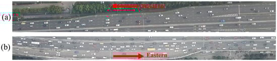
Figure 1.
Aerial view of the study area: (a) Western merging area and (b) Eastern merging area.
The western merging area has two datasets from different periods, named SQM1 and SQM2, while the eastern merging area has one dataset, named YT3. SQM1 has a sampling duration of 331 s, capturing the entire process from free flow to congested flow; SQM2 has a sampling duration of 842 s, mostly covering free flow and stable flow; and YT3 has a sampling duration of 514 s, entirely in congested flow.
We calculated the capacity drop and spatiotemporal characteristics of the two merging areas using Cassidy’s method [34]. Figure 2 presents the cumulative traffic flow curves (curves of O(t)) for the three datasets. The solid green line shows the cumulative flow at the Gore section, while the solid red line shows the flow at the End of Taper section. The red dashed line represents the actual capacity. It is the product of the cumulative flow curve slope at the End of Taper section and the background flow rate. The background flow rate , set as the critical capacity of 1650 pcu/ln/h for both merging areas, is derived from the Highway Capacity Manual (HCM). The capacity drop (CD) is calculated as the percentage difference between the actual and critical capacity.
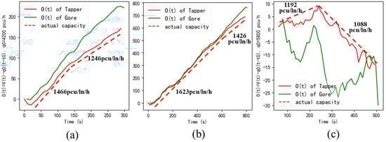
Figure 2.
O(t) at Gore and End of Taper sections for each dataset: (a) SQM1, (b) SQM2, and (c) YT3.
In Figure 2a, SQM1 shows a widening gap between the cumulative curves at 140 s. This indicates that the output flow rate is below the input flow rate, indicating the onset of congestion at 140 s. By the end of the dataset, SQM1’s actual capacity stabilizes at 1246 pcu/ln/h, resulting in a CD of 24.5%. In Figure 2b, SQM2 shows congestion starting at 600 s, with actual capacity stabilizing at 1426 pcu/ln/h and a CD of 13.5%. As shown in Figure 2c, YT3 experiences severe congestion from the beginning. At 240 s, the actual capacity stabilized at 1088 pcu/ln/h and a CD of 34.1%.
3.2. Variable Definition
The purpose of feature engineering is to generate and optimize predictor variables for analysis. This allows the model to better capture the effects of lane balance and imbalance designs on the dependent variable under traffic demand interactions. Thus, feature engineering focuses on transforming predictor variables and calculating interaction terms. The design of the interaction terms follows Zhao’s cross-level interaction variable method [17]. The geometric design factors and various traffic demand variables are multiplied to create the interaction terms. However, in practice, we found that categorizing lane balance as either 0 or 1 was too simplistic. This approach makes it difficult for the model to capture the distinct effects of each design under traffic demand. To solve this problem, we applied One-Hot Encoding. We represented the balanced design as [1, 0] and the unbalanced design as [0, 1]. This method reflects the interaction effects of the design schemes more accurately.
Table 2 shows all the variables used in the study and their statistical results. It includes both independent and dependent variables. The dependent variables are based on Hidas’ s driving behavior parameters for differentiating lane-changing types [10]. These parameters are also available in TESS NG. Lane change position parameters were obtained from Wan and Chen’s work, which verified the strong correlation between position and capacity using both empirical data and models [35,36]. The capacity drop calculation method follows Cassidy’s approach.
Table 2.
Description of variables.
We analyzed nine commonly used microscopic driving behavior parameters. These include lateral and longitudinal speeds, speed differential with the following vehicle during lane changes, acceleration difference, and LC_position. In order to reduce model complexity and select appropriate dependent variables, a correlation analysis was performed between the nine microscopic driving behavior parameters and the capacity drop (CD) metric. The results are shown in Figure 3.
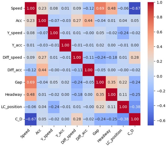
Figure 3.
Correlation matrix between driving behavior parameters and CD.
The correlation results show that Speed, Diff_speed, Gap, and LC_position have strong correlations with CD (>0.1). Among these variables, only Speed and Gap show a strong correlation with each other (0.69). Therefore, this study selects Speed, Diff_speed, and LC_position as dependent variables to analyze the impact of geometric design on microscopic driving behavior. Independent prediction models are developed for these variables.
4. Methodology
4.1. XGBoost
To study the impact of geometric design variables on microscopic driving behavior parameters under varying traffic demand conditions, a multilayer XGBoost model with cross-level interaction terms was developed. Compared to the standard XGBoost model, this multilayer design is more suitable for nested data, allowing for the simultaneous examination of variables from both levels on the dependent variables.
First, the basic expression of XGBoost can be represented as
In Equation (1), is the predicted value for the -th sample, representing the model’s output or target variable estimate, and K is the total number of trees, a hyperparameter that controls model complexity. is the prediction function of the -th tree, which is trained to approximate the target variable. Each tree’s function belongs to the function space . represents the feature vector for the -th sample, with each feature vector having dimensions ().
The function space in XGBoost is defined as follows:
In Equation (2), is the space of all possible functions for each tree. represents the prediction function, which outputs the weight for the leaf node assigned to input . The function maps each input to a specific leaf node in the tree, assigning it to one of the leaf nodes based on the feature space . is the total number of leaf nodes in each tree, where each node represents a unique region in the feature space. is the vector of weights for these leaf nodes, with as the prediction value of the leaf node to which input is assigned.
The objective function of the model is defined as
In Equation (3), is the loss function, which measures the difference between the predicted value and the actual value, and is the regularization term used to control the model complexity. The regularization term is defined as
In Equation (4), and are regularization parameters, is the number of leaf nodes, and is the weight of the -th leaf node. The objective function is optimized using an additive model optimization method, expressed as
By iteratively adding new functions to optimize the model, each iteration optimizes the current function and gradually reduces the value of the objective function. To compute the optimized value of the objective function, a second-order Taylor expansion is used, expressed as
where and are the first and second derivatives, respectively, calculated as follows:
Based on the basic model, interaction variables were added to the formula:
Equation (9) is used to calculate the change in the objective function before and after a split node to determine the optimal tree structure.
Interaction terms enhance the prediction accuracy by influencing the objective function optimization process (Equation (6)). By capturing the combined effects of traffic flow and geometric design variables (e.g., representing feature vectors), these interaction terms provide critical information that enables the model to identify the optimal split points during training. This process is directly supported by the split node optimization formula (Equation (9)), which calculates the change in the objective function before and after a split node.
During the iterative optimization of the objective function, the interaction terms participate in the computation of the first (, Equation (7)) and second derivatives (, Equation (8)) through a second-order Taylor expansion (Equation (6)). This derivative information is crucial for refining the model’s accuracy in each iteration. Incorporating interaction terms ultimately improves the model’s predictive ability for microscopic driving behaviors by allowing it to capture complex relationships that individual variables alone cannot represent. Consequently, this enhances the optimization of the weights () and structural parameters within the model (Equation (4)), leading to more accurate predictions.
Finally, the study evaluates the models using Root Mean Square Error (RMSE) and Explained Variance (Evar), comparing the predictive performance of the two models during the training and testing stages. The formulas for calculating the RMSE and Evar are as follows:
4.2. MOVES Model
The MOVES (Motor Vehicle Emission Simulator) model, created by the U.S. Environmental Protection Agency (EPA), is a key tool for estimating motor vehicle emissions [28]. The model calculates emissions for various pollutants through four distinct steps: First, the model processes vehicle operational data, such as the number of starts, running time, and idle time, to define the emission source. Second, the data are categorized by vehicle type and assigned to specific operating mode bins, with each bin representing a distinct emission process like evaporative, start-up, or running emissions. Third, the model computes emission rates (ER) using the emission process, vehicle type, and operating mode bin, while accounting for external factors such as fuel type and ambient conditions. Finally, the emission rates from the operating mode bins are adjusted by specific factors to calculate the total emissions. The formula for calculating the total emissions is as follows:
Here, represents the total emissions (g/h), is the total emissions for a specific pollutant (g/h), and is the adjustment factor for the emission process based on environmental conditions and fuel type.
The operating mode distribution serves as a central parameter for the emission calculations in this model. It categorizes different driving states—acceleration, deceleration, cruising, and idling—into distinct bins. The MOVES Model assigns vehicles to these bins based on the speed and acceleration recorded at precise time intervals. The vehicle’s specific power (VSP) is calculated at regular time intervals by inputting its instantaneous speed and acceleration into the formula, which identifies the corresponding operating mode bin. For further details, refer to the EPA’s literature [28].
For typical light-duty vehicles, the VSP calculation formula is as follows:
where is the instantaneous acceleration (m/s2), is the road slope (radians), and is the instantaneous speed (m/s).
For trucks, the VSP calculation formula is as follows:
where and are constants related to trucks, and is the gravitational acceleration (9.81 m/s2).
Vehicles are assigned to the corresponding operating mode bins using VSP values calculated at regular intervals. The emissions for various pollutants are calculated using the time distribution of these operating mode bins and the corresponding emission rates in the MOVES Model. The pollutants included in the calculation are carbon dioxide (CO2), nitrogen oxides (NOx), particulate matter (PM), volatile organic compounds (VOCs), carbon monoxide (CO), and sulfur oxides (SOx). The emission calculation depends on the time spent by the vehiclein different operating mode bins and the associated emission rates. The formula for calculating the emissions of each pollutant is as follows:
where represents the emission rate for a specific emission process, operating mode bin, and pollutant, measured in g/s. is the vehicle’s duration in a specific operating mode bin, measured in seconds.
This study utilizes vehicle trajectory data generated by simulation platforms to provide a more precise representation of the operating mode distribution in merging areas. These data are employed to calculate VSP values at regular intervals. The operating mode distribution is subsequently determined according to the definitions of the operating mode bin. The MOVES Model is then used to quantify the differences in total emissions under lane-balanced and imbalanced conditions, even when traffic demand and composition remain unchanged.
4.3. Calibration Method
The calibration process includes three tasks: evaluation metrics, sensitivity analysis, and calibration of sensitive parameters. It was recommended by Song et al. for TESS NG [37]. This method includes the calibration of the vehicle dynamics model, such as the maximum speed, maximum acceleration, deceleration, and variance for various vehicle types. It also includes calibration of the car-following and lane-changing models.
The evaluation metrics used are C1, C2, GEH, and DevS. According to Ban [38], C1 is an indicator that measures the spatial-temporal alignment of the bottleneck regions between the observed and simulated data.
where is a binary speed matrix based on , indicating whether a specific time and spatial location are in a congested state. represents the simulation value, and represents the real-world value. denotes the intersection, and denotes the union. represents the length of the merging area, which is the distance from the Gore point to the end of the acceleration lane. Both merging areas are 160 m long.
A higher C1 value indicates better alignment, and a value of C1 = 1 signifies a perfect match between the observed and simulated bottleneck regions.
C2, in addition to measuring the alignment of the bottleneck regions, also evaluates the match of speeds within these regions.
where represents the speed value of detector at time , is the simulated value, and is the actual value.
A value of C2 = 1 indicates that both the bottleneck region and speeds are perfectly matched between the observed and simulated data. Specifically, C2 is a stricter metric than C1, as it requires a speed match on top of the bottleneck alignment to achieve higher values.
GEH represents the alignment of traffic flow data between the simulation output and the observed data.
where is the section index, starting from the Gore point, with a virtual loop detector placed every 10 m. represents the simulation time step. is the flow rate of the simulation model, and is the observed flow matrix.
It is an empirical metric designed to compare two sets of flow data, where smaller values indicate better alignment.
DevS measures the alignment of speeds between simulation output and observed data. It represents the percentage of the relative speed error, which is calculated from the relative error matrix. In this study, all values in the matrix were sorted, and the worst 15% of the results were removed. The average of the remaining 85% of the data was used as the DevS metric.
Based on the studies by Song and Ban [37,38], the target thresholds for these metrics were set as follows: C1 > 0.7, C2 > 0.65, GEH < 5, and DevS < 15%.
TESS NG has 22 parameters for the car-following and lane-changing models, but not all parameters significantly affect the simulation results. TESS NG recommends using analysis of variance (ANOVA) to select sensitive parameters. The approach sets 10 random seeds and performs 10 simulations. Each simulation changes one parameter, resulting in 220 evaluation metrics. ANOVA can test the consistency of these evaluation metrics to determine whether a parameter significantly impacts the model. A p-value less than 0.05 is used to determine significance. All other parameters use the platform’s default values.
Calibration of the 9 sensitive parameters was performed using SPSS (v23) software. An orthogonal experiment L64(6^9) with nine factors and six levels was designed. TESS NG was iteratively run, and the simulation results were imported into SPSS. The parameters in the utility function were estimated using maximum likelihood estimation. The evaluation metrics were C1 and C2 maximization, GEH minimization (max 5), and DevS minimization (max 0.05).
5. Results and Discussion
5.1. Modeling Results
This study utilized three datasets (SQM1, SQM2, and YT3) from two merging areas, totaling 160,079 records. After cleaning, 80% of the data were assigned to the training set and 20% to the test set. Two feature sets were employed during model construction: one without interaction terms and one with. The first feature set included only the balance status and traffic volumes from the mainline and ramp (Vol_main, Vol_ramp, Vol_in). The second feature set added interaction terms between the lane balance status and traffic volumes, generating three additional features. Experiments were conducted using both feature sets, with the response variables being speed, speed differential, and lane-changing position, each treated independently. A logarithmic transformation was applied to smooth the distribution of the traffic flow variables, resulting in 128,063 records for training and 32,016 for testing. The XGBoost regression model was configured with 200 training rounds, a learning rate of 0.1, and a maximum depth of 5. The evaluation metric was the RMSE, with a random seed of 42, ensuring reproducibility.
Figure 4 shows the models’ learning curves over several training cycles, with the X-axis denoting the number of iterations and the Y-axis indicating the Root Mean Square Error (RMSE) of the three dependent variables. The results show that the XGBoost model effectively mitigates overfitting due to its built-in regularization. The introduction of interaction terms further reduced errors in both the training and testing phases, highlighting the enhanced generalization performance. Specifically, the prediction error for speed was reduced by 10%, the speed difference by 15%, and the lane-changing position by 18%.
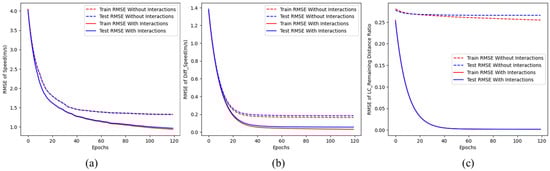
Figure 4.
Learning Curves for Each Prediction Model (a) Speed (b) Diff_speed, and (c) LC_Position.
We obtained the feature importance, impact direction, and significance of each variable in the three models (speed, speed differential, and lane-changing position) during training. Feature importance is evaluated using the split gain in the XGBoost model. The importance of each factor is determined by its contribution to reducing the model error during training. Features with higher importance significantly reduce errors and improve predictive performance. The impact direction is determined by the feature’s regression coefficient. A positive impact means that an increase in the feature raises the target variable. A negative impact means that an increase lowers the target variable. Significance is assessed indirectly by analyzing the impact of each feature on the model’s error. XGBoost does not conduct traditional significance tests (such as t-tests or F-tests). We assess feature importance and significance based on changes in the model’s training error. This reflects each feature’s contribution to the model’s predictive performance.
In each subplot of Figure 5, the vertical axis shows the importance from low-to-high. Positive impacts are shown in green and negative impacts are shown in red. High significance is shown with ‘***’. In the speed prediction model (Figure 5a), all traffic demand variables reduce the speed. Ramp flow has the largest effect. A higher traffic demand increases the negative impact on speed. The interaction between lane balance and traffic demand variables positively impacts speed. Lane balance has the lowest significance but shows a positive effect. In the speed differential model (Figure 5b), the interaction between the lane balance and traffic demand variables negatively impacts the speed differential. This means that the absolute value of the speed differential is smaller under lane balance. The interaction between the input flow and lane balance is more important than the other variables. Traffic demand variables increase the speed differential. Lane balance has the lowest significance and importance but shows a positive effect. In the lane-changing position model (Figure 5c), the mainline flow and the interaction between lane balance and input flow have the most significant impacts. Mainline flow has the highest importance and negative effect. A higher mainline flow makes vehicles more likely to change lanes at the end of the acceleration lane. The interaction between lane balance and input flow positively impacts the lane-changing position.
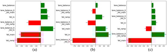
Figure 5.
Analysis of feature variable importance, impact direction, and significance for each model (a) speed, (b) Diff_speed, and (c) LC_Position.
Figure 6 shows the prediction results for the speed prediction model, speed differential prediction model, and lane-changing position prediction model. The horizontal axis represents the input flow rate, and the vertical axis represents the predicted values. Blue indicates the results for the lane-balanced design, while orange indicates the results for the lane-imbalanced design.
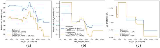
Figure 6.
Comparison of prediction results for each model: (a) speed, (b) Diff_speed, and (c) LC_Position.
The speed prediction results in Figure 6a show that the speed decreases as the input flow rate increases in both balanced and imbalanced scenarios. When the flow rate exceeds 1600 pcu/ln/h, speed drops sharply due to approaching the critical capacity of the downstream mainline in the merging area, indicating the onset of traffic congestion. Additionally, the balanced scenario shows an average speed of 17.15 m/s, while the imbalanced scenario averages 14.7 m/s, representing a 14.3% reduction.
In the speed differential prediction results in Figure 6b, positive values indicate that the speed of lane-changing vehicles is higher than that of the leading vehicle, typically occurring in free or cooperative lane-changing behaviors [23]. Negative values usually imply forced or aggressive lane-changing behavior [10]. The prediction results also show that under low (<750 pcu/ln/h) and high (>1600 pcu/ln/h) traffic flow conditions, the speed differential values for lane-balanced designs are significantly lower than those for lane-imbalanced designs. This suggests that forced lane-changing behaviors are more likely in lane-imbalanced scenarios, leading to more unstable traffic flows [10]. However, under medium traffic flow conditions, there is no significant difference in speed differentials between the balanced and imbalanced scenarios. This indicates that lane balance design has a smaller impact on speed differentials at medium flow levels.
The lane-changing position prediction results in Figure 6c show that as traffic demand increases, more vehicles tend to change lanes near the end of the acceleration lane. Under low and medium traffic flow conditions, there is little difference in the lane-changing positions between the two scenarios. When the flow rate exceeds 1600 pcu/ln/h, vehicles in imbalanced scenarios change lanes significantly closer to the end of the lane.
5.2. Calibration Results
Three simulation models were created: SQM1, SQM2, and YT3, based on the designs of the two merging areas in Figure 1. The designs of SQM1 and SQM2 are identical, with only the traffic flow requirements differing. The simulation durations are 331 s, 842 s, and 514 s. Calibration data for SQM1 and SQM2 were obtained from two datasets of the western merging area. Data from the eastern merging area were used to calibrate YT3.
Calibration includes three tasks: evaluation metrics, sensitivity analysis, and calibration of sensitive parameters. The target thresholds for the evaluation metrics were set as follows: C1 > 0.7, C2 > 0.65, GEH < 5, and DevS < 15%. When the simulation model meets these thresholds, its accuracy is considered acceptable.
The sensitivity analysis results show nine critical parameters that significantly affect the models. For the car-following model (IDM), the optimal parameters determined were the safe headway (s), stopping distance (m), α, and β. For the MLC model, the parameters are the minimum gap to the target lead vehicle β0 (m), target lead vehicle coefficient β1 (/(km/h)), target lead vehicle coefficient β3 (/(km/h)), and target following vehicle coefficient β2 (/(km/h)). For the FLC model, the minimum gap to the target lead vehicle β0 (m) was also found to be significant. All other parameters use the platform’s default values. The calibration results for the three models are presented in Table 3.
Table 3.
Calibration values for each model.
5.3. Simulation Results
5.3.1. Validation Experiment for Simulation Models
This experiment validates the proposed method’s ability to replicate traffic conditions at both the microscopic and macroscopic levels. Nine simulation models were created. The first type of model is the TESS NG Default model with default parameters. The second type of model is calibrated without XGBoost external control. The third type of model is calibrated with XGBoost external control.
Integrating the XGBoost model into TESS NG is straightforward. Following Lindorfer’s method, the XGBoost models focus on ramp vehicles, while other vehicles are handled automatically by the simulation model [9]. The XGBoost model includes three components: speed, lane change speed difference, and lane change position. Every 5 s, the XGBoost model receives flow data from TESS NG. It converts this data into flow rate and outputs the corresponding driving parameters. TESS NG uses these parameters to control the target vehicle’s desired speed, acceptable speed difference for lane change, and desired position. Ramp vehicles calculate the required lane change type based on the speed difference and gap. They then perform a lane change at the desired lane change position. If the vehicle determines that a safe lane change is not possible, it will cancel the lane change. The vehicle switches to the simulation platform control and waits for the next instruction.
Nine simulation models were validated against empirical observations using C1, C2, GEH, and DevS metrics calculated for each iteration. These metrics were then averaged per model, and the results are presented in Table 4. The Calibrated without Prediction Model configuration met or exceeded the predefined thresholds for all metrics, demonstrating a high degree of alignment with empirical observations. Calibrated with XGBoost, the model demonstrates higher performance across all metrics compared to both the TESS NG Default and the Calibrated without XGBoost configurations. Improvements are particularly notable in C1 and C2, along with consistent gains in GEH and DevS. XGBoost as an external control improves TESS NG’s capability to replicate traffic flows at both microscopic and macroscopic levels. This enhancement confirms the reliability of the proposed method.
Table 4.
Evaluation of metric results for each simulation model.
5.3.2. Lane Balance Design Control Experiment
Based on the validated Calibrated with XGBoost Models, we created three control experiment models to examine lane imbalance by shifting only the lane balance design while keeping all other geometric and traffic parameters constant. Based on the validated Calibrated with XGBoost Models, we created three control experiment models to examine lane imbalance by shifting only the lane balance design while keeping all other geometric and traffic parameters constant. Specifically, in the TESS NG interface, we directly modified the length of the outer ramp lane using a method similar to that of VISSIM. For example, in SQM1, the outer ramp lane in the merging area is originally terminated at the Gore point. We extended the endpoint of this lane to connect with the end of the taper of the Inter ramp lane, creating a lane imbalance in the merging area. The modification of SQM2 followed the same approach. For YT3, the outer ramp lane and the Inter ramp lane originally shared a taper. We shortened the outer ramp lane so that it connected with the Inter ramp lane before reaching the Gore point, thus shifting YT3 to a lane-balanced design.
To evaluate the merging area’s actual capacity under different lane balance designs, we set the random seed of these six simulation models to 0 and extracted their trajectory data. Using the End of Taper section as the actual capacity, we compared the O(t) for these six models against measured field data, following the same method in Figure 2. In Figure 7, the red solid line represents the measured data, the blue solid line represents simulation results without lane balance adjustments, and the green solid line shows the simulation results after shifting the lane balance design. Additionally, the blue dashed line and green dashed line correspond to the actual capacities before and after the lane balance shift, respectively.
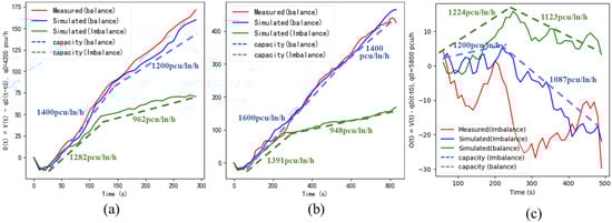
Figure 7.
Comparison of O(t) for each model: (a) SQM1, (b) SQM2, and (c) YT3.
All three Calibrated with XGBoost Models accurately replicated the full capacity drop (CD) process observed in their respective datasets. For SQM1, the capacity dropped to 1200 pcu/ln/h after 150 s, resulting in a CD of 27.3%. For SQM2, the capacity dropped to 1400 pcu/ln/h after 600 s, with a CD of 15.2%. For YT3, the capacity dropped to 1087 pcu/ln/h after 240 s, resulting in a CD of 34.1%.
After shifting to a lane-imbalanced design, both SQM1 and SQM2 showed a severe CD under the same traffic demand. For SQM1, the capacity dropped to 962 pcu/ln/h after 100 s, resulting in a CD of 41.7%, with more severe congestion. For SQM2, the capacity dropped to 948 pcu/ln/h after 220 s, leading to a CD of 42.5% and intensified congestion. Notably, despite the differences in traffic demand and composition, the extent of CD was similar for both models under the same geometric design conditions. After shifting to a balanced design, an improvement in the actual capacity was observed. YT3 showed a slight improvement in the actual capacity around 240 s, leading to a CD of 31.9%.
Controlled experiments indicate that lane imbalance decreases the merging area capacity. Congestion begins in imbalanced merging areas, even under lower traffic demand, and is more severe than that in balanced areas, as shown in Figure 6 and Figure 7. In the high-density traffic flow of YT3, optimizing the lane balance can slightly alleviate congestion. A possible reason is that frequent and complex lane changes in lane-imbalanced areas lower the speeds of acceleration lanes. Some vehicles may accept higher speed differences when changing lanes. This verifies Xue’s hypothesis [2]. Further analysis shows that capacity suddenly drops as traffic demand increases. A possible explanation is that in lane-imbalanced areas, when the traffic density reaches medium to high levels, most vehicles are forced to choose to change lanes near the end of the acceleration lane. This aligns with Chen and Wan’s findings [35,36]. Such lane-changing behavior further reduces the mainline traffic stability, leading to a sudden capacity decrease, as shown in Figure 7a,b.
The simulation results show that the proposed method is highly adaptable to changes in geometric design elements. Figure 7a,b reveals that changing the western merging area to a lane-imbalanced design caused similar capacity drops and severe congestion in SQM1 and SQM2, despite differences in traffic demand and vehicle composition. The actual capacities were close at 962 and 948 pcu/ln/h, respectively. These consistent findings confirm the method’s capability to identify and quantify the universal negative impacts of lane imbalance on traffic flow.
In contrast, the eastern merging area’s actual capacity was 1088 pcu/ln/h, which was over 10% higher than that of the western merging area. This suggests that certain geometric elements affecting the driving behavior parameters may not have been fully considered. To address this, XGBoost and TESS NG can be used to adjust geometric parameters (e.g., acceleration lane length, Gore angle, and lane width) and traffic conditions (e.g., traffic volume and vehicle composition). These adjustments enhance the reliability of the simulation models, enabling them to support design optimization for various merging areas.
5.4. Emissions Results
This study applies the MOVES Model to quantify emissions across the six simulation models outlined in the preceding subsection using high-resolution vehicle trajectory data. Each simulation model incorporates a distinct truck ratio. Emission estimates were derived from continuous measurements of vehicle speed and acceleration, as calculated using the MOVES Model. Table 5 details these findings, presenting the emissions in kg/h across the simulated scenarios.
Table 5.
Comparative emissions for pollutants under balanced and imbalanced lane designs across simulation models (Truck Proportions: SQM1—24%, SQM2—19.5%, YT3—9.4%).
YT3’s imbalanced design results in emission levels close to those of SQM1 and SQM2, which have higher truck proportions. Under imbalance, YT3’s CO2 emissions reach 495 kg/h, which is close to SQM1’s 550 kg/h and SQM2’s 545 kg/h. Similarly, YT3’s emissions of CO, NOx, and VOCs under the imbalance scenarios are nearly on par with SQM1 and SQM2. A comparison of the emissions under balanced and imbalanced lane designs within the same model reveals a significant increase in emissions. For example, SQM1’s CO2 emissions increased by 30.5%, SQM2’s by 33.6%, and YT3’s by 39.8%.
The emission results demonstrate that lane imbalance designs significantly increase emissions in the same merging area, even when the traffic demand and truck ratios remain constant. This effect likely stems from improper driving behaviors that emerge under specific traffic conditions. As shown in Figure 6, differences in the driving behavior parameters become notable when the traffic demand reaches medium levels (approximately 1300 pcu/ln/h). At this threshold, limited merging space in lane imbalance areas triggers frequent improper driving behaviors like acceleration, deceleration, and idling. According to previous studies by Liang and Yıldırım [5,6], these behaviors are key contributors to higher pollutant emissions under such conditions. To assist traffic management in mitigating congestion and emissions, we recommend implementing traffic flow guidance or ramp metering strategies before the traffic demand in merging areas reaches 1300 pcu/ln/h.
Another observation is that despite the low truck ratios in some merging areas, pollutant emissions remain close to those in merging areas with lane balance. This suggests that lane imbalance may amplify the pollution effects of trucks. However, this finding may also be influenced by the traffic flow state at YT3. The data for YT3 were collected during periods of severe congestion, resulting in stop-and-go conditions for all vehicles. The current dataset does not include traffic states prior to the onset of congestion. Expanding the dataset to capture additional traffic conditions would enable a more comprehensive analysis of the combined effects of lane imbalance and truck ratios on emissions.
The XGBoost model and simulation results show that lane balance design significantly improves capacity. This is achieved by reducing improper driving behaviors and enhancing the overall traffic flow stability. However, careful trade-offs are required, as the relationship between capacity and emissions varies under different designs. This is because the lane balance design’s impact on traffic flow may be limited under high traffic demand. Therefore, road design and traffic management must balance capacity, emissions, and traffic flow stability. Implementing lane balance design with proper traffic management measures (e.g., ramp metering and variable speed limits) can achieve multiple objectives, such as enhancing capacity, minimizing emissions, and improving traffic flow stability.
The observed reductions in emissions under lane-balanced designs have significant implications for broader environmental and sustainability objectives. By decreasing pollutants such as CO2, CO, NOₓ, and VOCs, lane balance design contributes to improving air quality and reducing urban air pollution. These improvements also contribute to meeting regional and national emission targets, aligning with global efforts to combat climate change and foster sustainable transportation systems. Therefore, implementing lane-balanced designs in expressway merging areas is not only an effective strategy for enhancing traffic efficiency but also a valuable approach to advancing environmental sustainability.
6. Conclusions and Future Work
Lane imbalance often leads to earlier and more severe congestion. This phenomenon occurs because lane imbalance does not provide sufficient space for stable lane-changing. When the traffic volume exceeds a certain threshold, it triggers more aggressive or unsafe driving behaviors, resulting in a rapid decline in actual capacity and a significant increase in pollutant emissions. To quantitatively analyze the effect of lane imbalance on road capacity and emissions, this study developed a driving behavior parameter prediction model based on XGBoost. This model can capture the complex nonlinear relationships among geometric design elements, traffic flow demand, and driving behavior parameters. This study built a controlled simulation environment for lane balance by integrating an adjusted XGBoost model.
The findings indicate that speeds in imbalanced areas consistently remain lower than those in balanced areas as traffic demand increases. When the traffic demand exceeds 1300 pcu/ln/h, drivers tend to make lane changes with larger speed differences and closer to the end of the acceleration lane. Under the same traffic demand, shifting the merging area design from lane balance to imbalance leads to an earlier and greater capacity drop. For example, when the westbound merging area shifts to an imbalanced lane design, the capacity drops from 27.3% and 15.2% to 41.7% and 34.1% in two datasets (SQM1 and SQM2). In another case, the severely congested eastbound merging area (YT3) with an imbalanced lane design showed a capacity drop from 34.1% to 31.9% after shifting to lane balance. Pollutant emission results indicate that imbalanced merging areas produce higher emissions than balanced designs. For instance, shifting to lane balance reduces YT3’s CO2 emissions by 39.8% from 495 kg/h. Shifting SQM1 and SQM2 to imbalanced lanes increases CO2 emissions by 30.5% and 33.6%, respectively.
In conclusion, we recommend that traffic engineers and policymakers prioritize lane balance in merging area design. The most cost-effective approach is to optimize road markings to ensure that the outer lane of the acceleration lanes merges with the inter lane before the Gore point. This method incurs the lowest cost and is likely to yield the greatest benefits. One critical consideration for the recommended solution is that the width of the acceleration lanes should not exceed 4 m [1]. When the lane width exceeds 4 m, it increases the likelihood of two vehicles traveling parallel within the single lane. This design can lead to a higher frequency of improper driving behavior. Meanwhile, if the lane balance design cannot be adjusted, ramp metering facilities on ramps can be introduced. Implementing ramp metering strategies before the traffic demand in merging areas reaches 1300 pcu/ln/h is advised. However, this approach incurs higher costs and may not outperform the first solution. In the future, merging area capacity and pollution reduction can be further improved by combining optimized designs, vehicle-to-infrastructure communication, and dynamic traffic management systems.
This study has two main limitations. The first is the small data sample. Hence, the results of the controlled simulation experimental model were not validated. For example, we did not find a merging area where SQM1 was altered to a lane imbalance for model calibration. Moreover, a larger data sample would improve model accuracy. Additional geometric factors, like Gore angle and acceleration lane length, should be considered. This would enable a more thorough analysis of how geometric factors affect CD and emissions. The second limitation arises from the way the MOVES Model was applied in this study, which could affect the accuracy of the emission estimates. For example, we only applied the MOVES Model’s distinction between passenger cars and heavy trucks without further specifying other vehicle types. Additionally, the study did not account for the proportion of new energy vehicles.
Future research will address these limitations. First, we collected UAV videos for over 35 min from seven merging areas on Guangzhou’s Inner Ring Expressway. The driving behavior parameter prediction model is expanded to include geometric factors, such as the acceleration lane length and the Gore angle. The second future work will be to examine the environmental impact of trucks as the geometric design changes. This involves further calibration of the MOVES Model and exploration of how changes in geometric design can reduce fuel consumption and congestion costs. Additionally, emerging technologies like vehicle-to-infrastructure communication and dynamic traffic management systems will be explored to enhance the applicability of the findings. Future research will align this study with sustainability goals, making it more relevant for traffic engineers and policymakers.
Author Contributions
Conceptualization, K.Z. and J.R.; Methodology, K.Z.; Software, Y.G. and K.Z.; Validation, K.Z., Y.G. and J.R.; Formal Analysis, K.Z.; Investigation, K.Z. and Y.C.; Resources, J.R.; Data Curation, Y.C.; Writing—original draft preparation, K.Z.; Writing—review and editing, K.Z., J.R. and Y.G.; Visualization, K.Z.; Supervision, J.R.; Project Administration, J.R. All authors have read and agreed to the published version of the manuscript.
Funding
This research received no external funding.
Institutional Review Board Statement
Not applicable.
Informed Consent Statement
Not applicable.
Data Availability Statement
Data are contained within the article.
Conflicts of Interest
The authors declare no conflicts of interest.
References
- American Association of State Highway and Transportation Officials (AASHTO). A Policy on Geometric Design of Highways and Streets, 7th ed.; American Association of State Highway and Transportation Officials: Washington, DC, USA, 2018; pp. 949–952. [Google Scholar]
- Xue, X.; Song, R.; Yan, K. Balance of Lanes Impacting Traffic Operation in Merging Area of Expressway On-Ramp. In Proceedings of the ICTE 2011, Chengdu, China, 23–25 July 2011. [Google Scholar] [CrossRef]
- National Cooperative Highway Research Program (NCHRP). Chapter 12 Interchanges. In Human Factors Guidelines for Roadway Designers and Traffic Engineers; NCHRP Report 600; Transportation Research Board: Washington, DC, USA, 2008; pp. 105–110. Available online: http://onlinepubs.trb.org/onlinepubs/nchrp/nchrp_rpt_600A.pdf (accessed on 10 November 2024).
- van Beinum, A.; Wegman, F. Design guidelines for turbulence in traffic on Dutch motorways. Accid. Anal. Prev. 2019, 132, 105285. [Google Scholar] [CrossRef] [PubMed]
- Liang, X.; Song, H.; Wu, G.; Guo, Y.; Zhang, S. Complex Traffic Flow Model for Analysis and Optimization of Fuel Consumption and Emissions at Large Roundabouts. Sustainability 2024, 16, 9464. [Google Scholar] [CrossRef]
- Yıldırım, Z.B.; Özuysal, M. Autonomous Vehicles and Urban Traffic Management for Sustainability: Impacts of Transition of Control and Dedicated Lanes. Sustainability 2024, 16, 8323. [Google Scholar] [CrossRef]
- Treiber, M.; Kesting, A. An open-source microscopic traffic simulator. IEEE Intell. Transp. Syst. Mag. 2010, 2, 6–13. [Google Scholar] [CrossRef]
- Nalic, D.; Pandurevic, A.; Eichberger, A.; Fellendorf, M.; Rogic, B. Software Framework for Testing of Automated Driving Systems in the Traffic Environment of Vissim. Energies 2021, 14, 3135. [Google Scholar] [CrossRef]
- Lindorfer, M.; Backfrieder, C.; Mecklenbräuker, C.; Ostermayer, G. Driver behavior injection in microscopic traffic simulations. In Modeling, Design and Simulation of Systems, Proceedings of the 17th Asia Simulation Conference, AsiaSim 2017, Melaka, Malaysia, 27–29 August 2017; Springer: Berlin/Heidelberg, Germany, 2017; pp. 237–248. [Google Scholar] [CrossRef]
- Hidas, P. Modelling Vehicle Interactions in Microscopic Simulation of Merging and Weaving. Transp. Res. Part C Emerg. Technol. 2005, 13, 37–62. [Google Scholar] [CrossRef]
- Chen, X.; Li, Z.; Yang, Y.; Qi, L.; Ke, R. High-resolution vehicle trajectory extraction and denoising from aerial videos. IEEE Trans. Intell. Transp. Syst. 2021, 22, 3190–3202. [Google Scholar] [CrossRef]
- Ubiquitous Traffic Eyes. Available online: http://seutraffic.com/ (accessed on 15 November 2024).
- Kalvapalli, S.P.K.; Chelliah, M. Analysis and prediction of city-scale transportation system using XGBoost technique. In Recent Developments in Machine Learning and Data Analytics: IC3 2018; Springer: Singapore, 2019. [Google Scholar] [CrossRef]
- Lahiri, S.; Gan, A.C.; Shen, Q. Using simulation to estimate speed improvements from simple ramp metering at on-ramp junction. In Proceedings of the Transportation Research Board Annual Meeting, Washington, DC, USA, 13–17 January 2002. [Google Scholar]
- Habtemichael, F.; Picado-Santos, L. Sensitivity analysis of VISSIM driver behavior parameters on safety of simulated vehicles and their interaction with operations of simulated traffic. In Proceedings of the Transportation Research Board Annual Meeting, Washington, DC, USA, 12–16 January 2013. [Google Scholar]
- Farah, H.; Daamen, W.; Hoogendoorn, S. How Do Drivers Negotiate Horizontal Ramp Curves in System Interchanges in the Netherlands? Saf. Sci. 2019, 119, 58–69. [Google Scholar] [CrossRef]
- Zhao, J.; Guo, Y.; Liu, P. Safety Impacts of Geometric Design on Freeway Segments with Closely Spaced Entrance and Exit Ramps. Accid. Anal. Prev. 2021, 163, 106461. [Google Scholar] [CrossRef]
- Yang, B.; Liu, P.; Chan, C.Y.; Xu, C.; Guo, Y. Identifying the Crash Characteristics on Freeway Segments Based on Different Ramp Influence Areas. Traffic Inj. Prev. 2019, 20, 386–391. [Google Scholar] [CrossRef]
- Zhang, Y.; Shi, X.; Zhang, S.; Abraham, A. A XGBoost-based lane change prediction on time series data using feature engineering for autopilot vehicles. IEEE Trans. Intell. Transp. Syst. 2022, 23, 19187–19200. [Google Scholar] [CrossRef]
- Ahmed, S.; Hossain, M.A.; Ray, S.K. A Study on Road Accident Prediction and Contributing Factors Using Explainable Machine Learning Models: Analysis and Performance. Transp. Res. Interdiscip. Perspect. 2023, 19, 100814. [Google Scholar] [CrossRef]
- Yang, Y.; Wang, K.; Yuan, Z.; Liu, D. Predicting Freeway Traffic Crash Severity Using XGBoost-Bayesian Network Model with Consideration of Features Interaction. J. Adv. Transp. 2022, 2022, 4257865. [Google Scholar] [CrossRef]
- Chen, C.; Liu, Z.; Wan, S.; Luan, J.; Pei, Q. Traffic Flow Prediction Based on Deep Learning in Internet of Vehicles. IEEE Trans. Intell. Transp. Syst. 2020, 22, 3776–3789. [Google Scholar] [CrossRef]
- Ahmed, K.I. Modeling Drivers’ Acceleration and Lane Changing Behavior. Master’s Thesis, Massachusetts Institute of Technology, Cambridge, MA, USA, 1999. Available online: https://dspace.mit.edu/handle/1721.1/9662 (accessed on 10 November 2024).
- Farrag, S.G.; El-Hansali, M.Y.; Yasar, A.U.H. A Microsimulation-Based Analysis for Driving Behavior Modelling on a Congested Expressway. J. Ambient. Intell. Humaniz. Comput. 2020, 11, 5857–5874. [Google Scholar] [CrossRef]
- Erdmann, J. SUMO’s Lane-Changing Model. In Modeling Mobility with Open Data. Lecture Notes in Mobility; Behrisch, M., Weber, M., Eds.; Springer: Cham, Switzerland, 2015. [Google Scholar] [CrossRef]
- Liu, Q.; Sun, J.; Tian, Y.; Xiong, L. Modeling and Simulation of Overtaking Events by Heterogeneous Non-Motorized Vehicles on Shared Roadway Segments. Simul. Model. Pract. Theory 2020, 103, 102072. [Google Scholar] [CrossRef]
- Perez, A.; Barros, A. Comparison of Mobile Source Emission Models Using Aggregated and Disaggregated Data. WIT Trans. Built Environ. 2009, 107, 553–563. [Google Scholar] [CrossRef]
- U.S. Environmental Protection Agency (EPA). Draft Motor Vehicle Emission Simulator (MOVES) 2009: Software Design and Reference Manual; U.S. Environmental Protection Agency, Office of Transportation and Air Quality: Washington, DC, USA, 2009. [Google Scholar]
- Xu, X.; Liu, H.; Anderson, J.; Xu, Y.; Hunter, M.; Rodgers, M.; Guensler, R. Estimating Project-Level Vehicle Emissions with VISSIM and MOVES-Matrix. Transp. Res. Rec. 2016, 2570, 107–117. [Google Scholar] [CrossRef]
- Abou-Senna, H.; Radwan, E.; Westerlund, K.; Cooper, C. Using a Traffic Simulation Model (VISSIM) with an Emissions Model (MOVES) to Predict Emissions from Vehicles on a Limited-Access Highway. J. Air Waste Manag. Assoc. 2013, 63, 819–831. [Google Scholar] [CrossRef]
- Guo, H.; Zhang, Q.; Shi, Y.; Wang, D. Evaluation of the International Vehicle Emission (IVE) Model with On-Road Remote Sensing Measurements. J. Environ. Sci. 2007, 19, 818–826. [Google Scholar] [CrossRef]
- Mądziel, M. Vehicle Emission Models and Traffic Simulators: A Review. Energies 2023, 16, 3941. [Google Scholar] [CrossRef]
- Wan, Q.; Peng, G.; Li, Z.; Inomata, F.H.T. Spatiotemporal Trajectory Characteristic Analysis for Traffic State Transition Prediction Near Expressway Merge Bottleneck. Transp. Res. Part C Emerg. Technol. 2020, 117, 102682. [Google Scholar] [CrossRef]
- Cassidy, M.J.; Bertini, R.L. Some Traffic Features at Freeway Bottlenecks. Transp. Res. Part B Methodol. 1999, 33, 25–42. [Google Scholar] [CrossRef]
- Wan, X.; Jin, P.J.; Gu, H.; Chen, X.; Ran, B. Modeling freeway merging in a weaving section as a sequential decision-making process. J. Transp. Eng. Part A Syst. 2017, 143, 5017002. [Google Scholar] [CrossRef]
- Chen, D.; Ahn, S. Capacity-drop at extended bottlenecks: Merge, diverge, and weave. Transp. Res. Part B Methodol. 2018, 108, 1–20. [Google Scholar] [CrossRef]
- Song, R.; Sun, J. Calibration of a Micro-Traffic Simulation Model with Respect to the Spatial-Temporal Evolution of Expressway On-Ramp Bottlenecks. Simulation 2016, 92, 535–546. [Google Scholar] [CrossRef]
- Ban, X.; Chu, L.; Benouar, H. Bottleneck Identification and Calibration for Corridor Management Planning. Transp. Res. Rec. 2007, 1999, 40–53. [Google Scholar] [CrossRef]
Disclaimer/Publisher’s Note: The statements, opinions and data contained in all publications are solely those of the individual author(s) and contributor(s) and not of MDPI and/or the editor(s). MDPI and/or the editor(s) disclaim responsibility for any injury to people or property resulting from any ideas, methods, instructions or products referred to in the content. |
© 2024 by the authors. Licensee MDPI, Basel, Switzerland. This article is an open access article distributed under the terms and conditions of the Creative Commons Attribution (CC BY) license (https://creativecommons.org/licenses/by/4.0/).