Abstract
Power systems are the main source of carbon emissions. Currently, coordinated operation strategies of the source–grid–load–storage model considering carbon emissions is primarily expanded from the generation side. For practical power systems, where multiple types of generating units coexist at a single node, it is difficult to develop unit combination strategies that simultaneously consider carbon emission factors and power flow constraints. Therefore, a new power flow calculation method based on connectivity matrix theory was proposed, aiming to address the issues of existing approaches that are too coarse and unable to accurately represent the operating states of multiple units under each node. Furthermore, a new method for dynamic calculation of regional carbon emission based on connectivity matrix and carbon emissions flow was introduced to improve the accuracy of carbon emission measurements. Firstly, a simulation model for a coordinated optimization operation based on the minimum system cost for the source–grid–load was established and an optimal flow calculation method using a connectivity matrix was introduced. Second, a dynamic carbon emission calculation method, considering electricity sources, was developed by combining the results of the optimal power flow calculation with carbon emission flow theory. Finally, the effectiveness of the approach in this article was verified by the IEEE 14-bus system example and a provincial power grid, ensuring strict adherence to the conservation principle of carbon emissions between the supply and demand sides and satisfying power flow constraints.
1. Introduction
Most countries worldwide have reached a consensus on achieving ‘carbon peaking and carbon neutrality’ [1]. China has proposed accelerating the construction of a new type of power system to support the realization of the ‘carbon peaking and carbon neutrality’ goals. In the process of building the new power system, the focus is on increasing the proportion of clean energy and improving system efficiency to reduce carbon dioxide emissions from the source and process [2]. By the end of 2023, China’s cumulative installed capacity of grid-connected wind power and photovoltaic generation reached 1.05 billion kilowatts, accounting for 36% of the total installed capacity [3]. The scale of renewable energy generation has historically exceeded thermal power, with the annual increase exceeding half of the global total. However, with the promotion of electrification, it is estimated that by 2030, the proportion of load demand from end-use sectors such as industry, construction, and transportation through electrification will reach approximately 35% [4]. The power system load will continue to increase, and the task of achieving ‘carbon peak and carbon neutrality’ remains challenging [5].
The efficiency and accuracy of current carbon emission accounting techniques need improvement, and there is a lack of mature standards and unified measurement methods for carbon emission certification. Currently, carbon emission accounting methods mainly include macroscopic statistical methods [6], emission factor methods [7], mass balance methods [8], online monitoring methods [9], life cycle assessment methods [10], and carbon emission flow methods [11,12]. The carbon emission statistical accounting process highly relies on original production data and is currently limited to annual statistical calculations. The macroscopic statistical methods do not consider the specific technical processes of power system generation and require long-term fuel consumption statistics as data support, making it difficult to achieve detailed analysis of carbon emissions in power systems. The life cycle assessment methods analyze carbon emissions from a timeline perspective but lack consideration of the physical characteristics of power systems and cannot clarify the spatial–temporal transfer mechanisms of carbon emissions in the power system [13]. Emission factor methods, mass balance methods, and life cycle assessment methods are influenced by the statistical cycles of basic production data, such as fuel and raw materials, typically conducted on an annual basis. Online monitoring methods are currently the only means for continuous carbon emission monitoring, but due to economic and data reliability reasons, they have not been widely applied domestically. Carbon emission flow methods consider the transfer network of carbon emissions, bridging the gap between production and consumption, and can clarify carbon emission responsibilities [14,15]. However, they are still in the preliminary research stage and require further exploration. Additionally, the current carbon emission measurement methods cannot provide real-time guidance for the scheduling and operation of power plant units within the system.
To refine the strategy for a low-carbon target in the source–grid–load–storage system during its operational phase, the current simulation calculations that consider carbon emission flows [16] typically focus on several optimization objectives. These include minimizing system operation and maintenance costs [17,18], adhering to low carbon and system reliability constraints [19], reducing power losses [20], ensuring power balance [21], managing power flow [22], maintaining adequate system spinning reserves [23], optimizing power generation [24], and integrating energy storage systems [25]. However, these approaches often overlook the adequacy of system generation capacity. In addition, a coordinated low-carbon economic dispatch strategy is proposed in the article [26]. This strategy considers a dual-layer incentive-based carbon trading mechanism and provides a comprehensive energy optimization scheme for multi-agent systems with the park as the main agent. However, it does not guide the coordinated output of various types of power sources at individual nodes. Another paper [27] establishes a two-stage low-carbon dispatch model based on super-carbon demand response, which can effectively reduce system carbon emissions by shifting loads from high-carbon periods. However, it lacks optimization of the start-up combination of traditional units. Additionally, a power system carbon emission flow calculation method based on the power flow distribution matrix in the article [22] quantifies the carbon emissions sources and composition at each node. However, it lacks coordination optimization for the entire source–grid–load process, which prevents guidance on the coordinated output of various types of power sources. Paper [28] considers incentive loads, joint operation modes, and gas network characteristics to establish a low-carbon economic dispatch model for the electric–gas interconnected system, minimizing daily operating costs. While it provides the total output of multiple power sources at the system level. The feature of carbon emission calculation methods in other different literature is shown as Table 1. It can be seen that none of the mentioned studies offer guidance on the coordinated output combination for various types of units at individual nodes. Optimizing the coordinated output of diverse unit combinations directly impacts the size of carbon emission sources and is crucial for achieving safe and low-carbon operation in modern power systems. Therefore, analyzing the coordinated output combination of multiple types of units under each node is crucial.

Table 1.
Carbon emission calculation methods in different literature.
In response to the above issue, this paper incorporates various types of power generation units under the nodes into actual operational simulations using a connectivity matrix. By combining optimal power flow and carbon emission flow theories, the paper provides recommendations for combining multiple types of units under a low-carbon objective. Firstly, an optimal power flow calculation method (OPFCM) based on the connectivity matrix is proposed, and a simulation model for coordinated optimization of source–grid–load–storage is established based on minimizing system costs. Secondly, a dynamic carbon emission calculation method is introduced based on carbon emission flow theory and OPFCM. Finally, an in-depth analysis is conducted on the accuracy of system flow, reasonableness of unit output, and carbon emission conservation in both the IEEE 30-bus system and a provincial-level power grid system, validating the effectiveness of the proposed methods.
2. Calculation Method of Power Flow and Carbon Emission Flow Based on Chain Matrix
The calculation method for carbon emission flow in the power system [16] provides a comprehensive approach to our study [16]. Through the operating simulation calculations, the output of various types of generating units at each moment can be obtained, resulting in the branch power flow distribution matrix , the generator injection distribution matrix , the load distribution matrix , the demand response distribution matrix , the load shedding distribution matrix , and the renewable energy curtailment distribution matrix . To calculate the carbon flow and carbon potential introduced by each branch, the branch power flow distribution matrix undergoes element filtering, only retaining the power of the branches with power out flow. That is, when the power flow from node i to node j, PBij = p, PBji = 0.
The calculation of the node active flux matrix involves assessing the electric energy sources flowing into each node at various time intervals, along with their corresponding carbon emission factors. A node active power flux matrix is established to represent the sum of active power flowing into each node at each moment, which is an N-dimensional square matrix, denoted as , specifically, it is a diagonal matrix expressed as , whose diagonal elements calculation methods are as follows:
The calculation of the generator carbon emission factor matrix: assuming that the carbon emission factor for the generator() is denoted as , the generator carbon emission factor matrix can be represented as follows:
The calculation of the node carbon potential matrix: defining the carbon potential at each node as the average carbon emission obtained by distributing all carbon emissions flowing into that node over the total power flowing into the node. The node carbon potential matrix, denoted as , is an N × 1 matrix, and its elements are calculated as follows:
where represents the flow from node n to node i, and denotes the average carbon potential at node n. Additionally, represents the generator connected to node i, and corresponds to the carbon emission factor associated with that generator.
The calculation of the node carbon emission matrix aims to characterize the carbon emissions corresponding to the electricity consumption of loads at each node. The node carbon emission matrix, denoted as , is an M × 1 matrix, expressed as follows:
3. Simulation Models for New-Generation Power Systems Operation
Assuming a system with N nodes, including K power nodes (comprising generalized power sources such as coal-fired, gas-fired, wind, photovoltaic, and energy storage and so on), M load nodes, and L renewable energy nodes that experience power curtailment (primarily wind power and photovoltaic), the calculation flowchart for the carbon emission factors and carbon emissions in a multi-node system is illustrated as Figure 1:
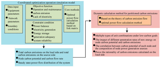
Figure 1.
Carbon emission factors and carbon emission calculation process for multi-node systems.
3.1. Establishment of the Target Function
In the operational simulation system of the new-type power system, it is essential to consider the economy, low carbon, and reliability of the system’s operation. Therefore, considering the system’s maintenance costs, carbon emission costs, and the cost of power shortages, the objective function for the operational simulation model is established as follows [17]:
where donate to the system’s maintenance costs, system’s carbon emission costs, and the cost of power shortages.
3.1.1. System’s Maintenance Costs
The calculation methods of system’s maintenance costs are as follows [18]:
where COM represents the fixed operation and maintenance costs required by the equipment loss and normal operation of the generating units, demand-side response, and energy storage; denotes the generation cost of the units; indicates the start-up and shut-down costs of the units; is the operational cost for demand-side response; and signifies the operational cost of the energy storage. , , , and , respectively, represent the operation and maintenance costs corresponding to the unit capacity of conventional units, the unit capacity of demand-side response, the unit power, and the unit capacity for energy storage. denotes the operating duration of the corresponding entity. , , and are the generation cost coefficients for conventional units. is the power generated by conventional units at time t, represents the start-up and shut-down state of the units, where = 1 indicates that the unit is operational at time t, and = 0 indicates that the unit is shut down at time t. and , respectively, represent the start-up and shut-down costs per unit capacity for conventional units. and , respectively, denote the start-up and shut-down actions of the units at time t, where = 1 indicates that the unit starts up at time t. = 1 indicates that the unit shuts down at time t, and = 0 or = 0 indicates that there is no change in the state of the unit at time t. represents the unit power operation and maintenance cost for demand-side response at time t, which is mainly reflected in the unit power opportunity cost loss due to the inability to participate in other auxiliary service markets after participating in the electricity quantity market balance. is the adjustment power of demand-side response at time t, and denotes the unit power cost of energy storage at time t, primarily reflecting the unit power cost caused by charge–discharge efficiency loss during energy storage discharge, which can be characterized by the average electricity price during energy storage charging. is the discharge power of energy storage at time t, and represents the charge–discharge efficiency of energy storage, which can generally be taken 86% as a certain value [18].
3.1.2. Annual Carbon Emission Cost of System
The annual carbon emission cost of the system is mainly related to the power generation of conventional units such as coal power and gas power in the system. The calculation method for the annual carbon emission cost of the system is as follows [19]:
where represents the penalty cost corresponding to the unit carbon emission, which can be characterized by the carbon trading price. For reference, the closing price of the national carbon market on 20 June 2022, was CNY 59.25 per ton CO2. denotes the operating duration of unit g, and represents the carbon emission factor of unit g. The typical power generation carbon emission factors for various types of units are shown in Table 2 [41,42].
Table 2.
The typical carbon emission factors for various types of power generation units.
3.1.3. The Cost of Power Shortage Loss
The cost of power shortage loss is mainly caused by the system’s inability to guarantee the basic electricity demand of users due to emergencies. The calculation method is as follows [20]:
where represents the penalty cost per unit of unserved energy. It can be initially characterized by the degree of electricity GDP, which is obtained by combining the annual GDP of the region and the total electricity consumption of the whole society. In this context, it is taken as 16.41 CNY/kWh. represents the duration of power outage for the load m connected through node i. represents the power outage of the load m connected through node i at time t.
3.2. Constraint Conditions
3.2.1. Power Balance Constraint
Considering that all nodes need to satisfy the power balance constraint at every moment, the power balance constraint of each node can be described as follows: at any moment, the power flowing into node i + the power generation of the generator connected to node i + the load response power of node i + the power shortage of the load at node i = the load power connected to node i + the power flowing out from node i + the discarded power of the renewable energy connected to node i. The mathematical expression is as follows [21]:
where represents the power flowing into node i from node n. donates the power generated by generator k connected at node i. refers to the adjustable depth of generator k connected at node i. According to the “Notice on Carrying out the Upgrading of Coal-fired Power Units Nationwide” issued by the National Development and Reform Commission and the National Energy Administration in 2021, the adjustable depth of coal-fired power units is taken as 0~35%; represents the response power of demand response m connected at node i, donates to the power shortage of load m connected at node i, refers to the power consumption of load m connected at node i, represents the power flowing out of node i to node n, and donates to the wasted power of renewable energy l connected at node i. The above system balance matrix can be further expanded and applied to calculate the power balance of each node in a multi-node system. For a multi-node system, a branch power flow distribution matrix, a unit injection distribution matrix, a load distribution matrix, a demand-side response distribution matrix, a load power shortage distribution matrix, and a renewable energy waste distribution matrix can be established, as shown below [15]:
- (1)
- Branch Power Flow Distribution Matrix
First, establish the branch power flow distribution matrix, which is an N-dimensional square matrix denoted as ; since the power flow between non-adjacent nodes is 0, the optimization result cannot consider the connection relationship between nodes, and there may be power flow between non-adjacent nodes. Therefore, a connectivity matrix needs to be defined and multiplied with the pre-optimized branch power flow distribution matrix to eliminate the power flow between non-adjacent nodes, and only the power flow between adjacent nodes is retained for the model optimization solution. The branch power flow connectivity matrix is also an N-order square matrix, denoted as , if there is a branch connected between node i and node j (i, j = 1, 2, …, N); hence, = 1, = −1, and the branch power flow distribution matrix is equal to the product of the branch current connectivity matrix multiplied by the branch current pre-distribution matrix. The mathematical expression is as follows [16]:
where is the N × N branch power flow pre-distribution matrix obtained by system optimization, and is the branch power flow distribution matrix. If there is a branch connected between node i and node j (i, j = 1, 2, …, N), and the positive active current p flows from node i to node j through this branch, then = p, = −p; if the active current p flowing through this branch is a reverse current, then = −p, = p; in other cases, = = 0, specifically, for all diagonal elements, = 0(i, j = 1, 2, …, N).
- (2)
- Unit Injection Distribution Matrix
The unit injection distribution matrix is a K × N order matrix, denoted by . If the kth (k = 1, 2, …, K) power generating unit is connected to node j, and the active current injected from the kth node containing a generator to node j is p, then = p; otherwise, = 0. Since the unit injection pre-distribution matrix obtained by optimization may yield output values at nodes where generator unit k is not connected, it is necessary to correct the unit injection pre-distribution matrix with the unit connectivity matrix. The unit connectivity matrix is denoted by , and if generator unit k is connected to node j (j = 1, 2, …, N), then = 1. The relationship between the unit injection distribution matrix and the connectivity matrix is as follows:
Since one unit can only inject into one node, there is the following constraint for any row of the unit injection distribution matrix: only one element in (j = 1, 2, …, N) is non-zero; that is, the element corresponding to the column of the access point of unit i is non-zero, and the elements of the other N-1 columns are zero. The mathematical expression is as follows:
where represents the element in the kth row and jth column of the unit connectivity matrix; if generator unit k is connected to node j (j = 1, 2, …, N), then = 1; otherwise, it is 0.
- (3)
- Load Distribution Matrix
The load distribution matrix is an M × N order matrix denoted by If node j is the mth (m = 1, 2, …, M) node with load, and the active load is p, then = p; otherwise, = 0. Since the load data are an input boundary condition, there is no need to constrain them with a connectivity matrix. As one load can only be injected into one node, there is the following constraint for any row in the load distribution matrix, which means that only one element in (j = 1, 2, …, N) is non-zero, the element at the access point of load i is non-zero, and the other N-1 elements are all zero.
- (4)
- Demand-side Response Distribution Matrix
The demand-side response distribution matrix is an M × N order matrix denoted by . If node j is the mth (m = 1, 2, …, M) node with demand-side response, and the demand-side response adjustment power is p, then ; otherwise, it is . Since the demand-side response pre-distribution matrix obtained through optimization may result in output values in nodes where demand-side response m is not connected, it is necessary to correct the demand-side response pre-distribution matrix with the load connectivity matrix. The load connectivity matrix is denoted by , and if demand-side response m is connected to node j (j = 1, 2, …, N), then = 1. The relationship between the demand-side response distribution matrix and the connectivity matrix is as follows:
Since one demand-side response can only be connected to one node, there is the following constraint for any row of the demand-side response distribution matrix: only one element in is non-zero; that is, the element corresponding to the column of the access point of demand-side response m is non-zero, and the elements of the other N-1 columns are all zero. The mathematical expression is:
where represents the connection relationship between demand-side response m and node j (j = 1, 2, …, N); if demand-side response m is connected to node j (j = 1, 2, …, N), then = 1; otherwise, it is 0.
- (5)
- Load Power Shortage Distribution Matrix
The load power shortage distribution matrix is an M × N order matrix denoted by . If node j is the mth (m = 1, 2, …, M) node experiencing a power shortage, and the power shortage is p, then ; otherwise, it is . Due to the possibility of obtaining power outage values in nodes that are not connected to load m in the pre-distribution matrix of load power outage obtained through optimization, it is necessary to correct the load power shortage pre-distribution matrix using the load connectivity matrix. The relationship between the load power shortage distribution matrix and the connectivity matrix is as follows:
- (6)
- Renewable energy curtailment distribution matrix
The renewable energy curtailment distribution matrix is an L × N order matrix denoted by . If node j is the lth (l = 1, 2, …, L) node with renewable energy curtailment, and the curtailment power is p, then ; otherwise, it is . Since the renewable energy curtailment pre-distribution matrix obtained by optimization may yield curtailment values at nodes where renewable energy l is not connected, it is necessary to correct the renewable energy curtailment pre-distribution matrix with the renewable energy connectivity matrix. The renewable energy connectivity matrix is denoted by , and if renewable energy l is connected to node j (j = 1, 2, …, N), then = 1. The relationship between the demand-side response distribution matrix and the connectivity matrix is as follows:
Since a renewable energy plant can only curtail at the node it is connected to, there is the following constraint for any row of the renewable energy curtailment distribution matrix: only one element in (j = 1, 2, …, N) is non-zero, meaning the element corresponding to the column of the access point of renewable energy l is non-zero, and the elements of the other N − 1 columns are zero. The mathematical expression is as follows:
where represents the connection relationship between the renewable energy source l and node j (j = 1, 2, …, N); if the renewable energy source l with curtailment is connected to node j (j = 1, 2, …, N), then = 1; otherwise, it is 0.
3.2.2. System Power Flow Constraints
To further introduce the direct current flow to describe the flow constraints between nodes [22], the system node matrix and the system impedance matrix are established. represents the phase angle deviation of node i relative to the balance node, and characterizes the reciprocal of the admittance between node i and j. Then, the system flow constraints are represented as follows:
3.2.3. System Spinning Reserve Constraints
Considering the uncertainty of wind power and photovoltaic output, the system needs to consider satisfying the load demand with non-renewable energy sources during unit dispatch optimization. Therefore, the startup of non-renewable energy sources in the system need to meet the following constraint [23]:
where represents the maximum power generation capacity of generator unit k connected at node i, refers to the system load reserve rate, which is generally set at 2% to 3%. donates the power consumption of load m connected at node i, and represents the curtailed power of renewable energy source l connected at node i.
3.2.4. Constraints on Power Generation Technology
The constraints on power generation technology mainly include the output constraints of renewable energy units, the technical constraints of the conventional units’ output, and so on. For renewable energy units (such as wind power and photovoltaic), their operational constraints primarily depend on the availability of resources, and their maximum dispatchable capacity is represented as the product of the maximum capacity factor and the installed capacity. The above constraints are expressed as follows [24]:
where represents the set of conventional units, including coal-fired and gas-fired units, and refers to the set of renewable energy units, including wind power and photovoltaic generation units; and , respectively, donate the minimum and maximum technical output levels of the units; and , respectively, represent the maximum upward and downward ramping capabilities of the units, excluding the minimum output level required when the unit transitions from shutdown state to startup state; and , respectively, refer to the minimum continuous operating and shutdown time of the units; is the predicted energy factor of the renewable energy units. Constraint (20) represents the upper and lower limits of the output of conventional units; constraint (21) represents the ramping constraints of the units, with the downward ramping constraint being active when the unit transitions from a startup state to a shutdown state, and vice versa for the upward ramping constraint; constraints (22) and (23) indicate that the operating state and state transition flag of the units are both 0–1 variables, and restrict the units to have only one operating state at any given time; constraint (24) limits the minimum continuous startup time of the units; constraint (25) limits the minimum continuous shutdown time of the units; and constraint (26) limits the maximum and minimum output of renewable energy units.
3.2.5. Constraints of an Energy Storage System
The charging and discharging process of the energy storage system (ESS) must consider physical constraints such as energy storage charging and discharging efficiency, power constraints, and rated capacity constraints [25].
where represents the energy state of the energy storage; refers to the time interval. Constraint (27) represents the energy evolution process of the ESS. Constraint (28) represents the power constraints for charging and discharging of the ESS. Constraint (29) represents the upper and lower capacity constraints of the ESS. Constraint (30) ensures that the initial and final energy states of the ESS are equal over the optimization period [1,T].
3.2.6. System Generation Adequacy Constraint
The adequacy of a power system refers to its ability to meet user demand in terms of power generation, transmission, and supply after considering factors such as the outage or underperformance of some equipment, which characterizes the steady-state performance of the system. In the planning of traditional power sources, the planning target is usually set at a certain percentage higher than the annual peak load [43]. However, due to the volatility and randomness of renewable energy output, it does not possess the strong controllability of traditional thermal power units, and its generation adequacy differs significantly from conventional thermal power units. Traditional power system planning often neglects or simplifies the capacity value of renewable energy, leading to underinvestment or overinvestment in scenarios with a high proportion of renewable energy. Therefore, scholars have proposed the concept of capacity credit [44] (expressed as a percentage), which represents the proportion of wind and photovoltaic units that can be considered equivalent to conventional units under the premise of equal reliability, enabling the comparison of uncontrollable, volatile, and random generation technologies with conventional units on the same level. The system generation adequacy constraint is expressed as follows [45]:
In the formula, is the capacity credit coefficient of generators; is the capacity credit coefficient of energy storage, where the credible capacity of energy storage is related to the rated discharge duration. Energy storage can be used to replace traditional peaking power units, and its capacity credit is related to the maximum discharge duration of the energy storage. According to years of historical operational data from the California electricity market in the United States, the capacity credit of energy storage batteries with a discharge duration of 4 h is approximately about 75% [46]. is the system generation adequacy coefficient. Considering the possible faults or maintenance of the generator units in the system, the actual planned generation capacity should exceed a certain proportion of the system’s peak load. represents the power demand of important load z at time t, and Z represents the set of important loads.
3.2.7. System Reliability Constraint
The system reliability constraint is described through the load capacity shortage rate, ensuring that in emergency scenarios such as isolated operation of local microgrids, emergency power support can be provided to critical loads through internal distributed energy storage [19]. The constraint is expressed as follows:
where represents the remaining energy of storage s at time t; denotes the charging and discharging efficiency of the storage, which is generally around 86%; indicates the important load amount at node I; is the power supply guarantee coefficient for important loads, meaning the proportion of the important load that the remaining energy of the storage at the node should cover at any time, which is generally around 5%.
4. Instance Application Results
4.1. IEEE 14-Bus System
4.1.1. Verification of Optimal Power Flow Accuracy Based on Node Connectivity Matrix
To verify the accurate calculation of system power flow and carbon potential using the algorithm proposed, a comparative analysis was conducted with the IEEE 14-bus system and the literature [16], and present the calculation deviation percentage of key parameters in flowing table. The steady-state active power flow of the IEEE 14-bus system is shown in Appendix A, and the related system parameters are shown in Table 3.
Table 3.
Power flow comparison of the IEEE 14-bus system.
Based on the above analysis, it can be seen that the error of the active power flow of each branch obtained through the proposed optimal power flow calculation method based on the node connectivity matrix does not exceed 0.23%. This indicates that the proposed method can accurately calculate the system branch power flow, and the results are consistent with the AC power flow calculation results from Matpower, verifying the accuracy of the proposed algorithm.
4.1.2. Verification of Carbon Emission Accuracy Based on Node Linkage Matrix
By combining the active power flux of each node obtained from the optimal power flow calculation with the theoretical carbon emission flow, the carbon potential of each node can be obtained, as shown in Table 4.
Table 4.
Nodal active power flux and nodal carbon intensity of IEEE 14-bus system.
Through the proposed carbon potential calculation based on the linkage matrix, the active power flux of each node is consistent with the case study, with a carbon potential error of no more than 0.02%. This not only accurately reflects the active power flowing into each node of the system but also accurately reflects the carbon emission factors corresponding to the electricity consumption of each node, which is conducive to reasonably allocating the carbon emissions from the power supply side to each node.
4.1.3. Verification of Carbon Emission Conservation Based on Node Linkage Matrix
Further, by combining the carbon potential of each node with the power generation and load electricity consumption, the comparison of the load carbon flow rate of each node can be obtained, as shown in Table 5.
Table 5.
Load carbon emission rate of IEEE 14-bus system.
Based on the above analysis, it is known that the total carbon emissions from the load side obtained through the proposed dynamic calculation method for regional carbon emissions based on the linkage matrix are consistent with the total carbon emissions from the source side, indicating the proposed method can effectively measure carbon emissions from the load side. Furthermore, as can be seen from the table above, the traditional method of calculating carbon emissions from the source side based on carbon emission factors cannot account for the carbon emissions corresponding to different electricity consumption. For example, the electricity consumption of Node 3 is significantly higher than other nodes, but the carbon emissions calculated from the source side cannot reflect the actual carbon emissions caused by the real electricity consumption at this node. Therefore, it is necessary to carry out regional carbon emission calculations based on the connectivity matrix to calculate and verify the actual carbon emissions corresponding to the load electricity consumption of each node.
4.2. Actual Provincial System
To verify the rationality of the coordinated output of various types of generating units under each node under the premise of satisfying the safe and stable operation of the power system, a 21-node system composed of various cities in a province was selected as a case study. Its topological structure and power source composition are shown in Figure 2. The bold horizontal lines in the figure represent the busbars of each node, and the numbers next to the busbars represent the node numbers. The numbers in the colored circles correspond to the nodes where each unit is located. The output of wind power and photovoltaic at each node, and the system parameters are shown in Appendix A.
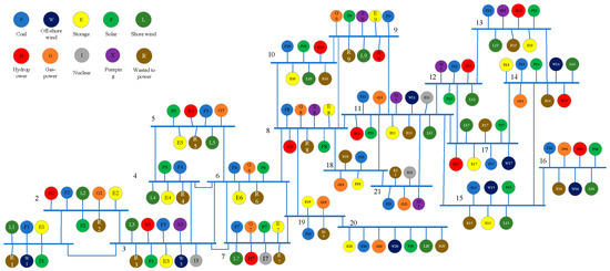
Figure 2.
Topology structure and power source composition of the 21-node system.
4.2.1. Analysis of Generating Unit Output Combination Characteristics
Through the new power system operation simulation based on the linkage matrix, the output of various types of power generating units in the system can be obtained as shown in Figure 3 and Table 6.

Figure 3.
Output of various power supply units of a provincial system on a typical day.
Table 6.
Carbon potential, carbon emissions, and energy composition at each node.
Through the system operation simulation, it is known that the system load is mainly met by coal power, nuclear power, imported electricity, and renewable energy. During the day from 9:00 to 12:00, due to the significant increase in imported electricity from outside the region, the energy storage begins to charge; to ensure that the amount of electricity at the starting and ending times is equal, the energy storage discharges from 22:00 to 24:00 to meet the load electricity demand. The operating status of other types of power sources also meets the corresponding constraints and is consistent with the actual operating status. To verify the rationality of the established generating unit output combination, the output status of various types of units is represented graphically, as shown in Figure 4.

Figure 4.
Analysis of output characteristics of typical power supply units: (a) coal-fired power units; (b) gas-fired power units.
In Figure 4, the horizontal axis represents the numbers of different types of generating units, and the vertical axis indicates the operating status of the units at each moment (one point every 15 min). The gradual change in colors in the figure represents the output status of the units, with dark blue indicating a shutdown state, and yellow indicating a state of full output. As can be seen from Figure 4a, by analyzing the output status of each unit at each moment, it is known that coal-fired power units have low operating costs, but due to their high carbon emission factors, there are fewer units operating at full capacity for extended periods. The reason why most units operate at a lower status for most of the time is due to line transmission constraints, thus requiring some units to maintain a lower output status. Further attention to the shutdown and continuous operation time of the units reveals that they all meet the start–stop constraints and ramping constraints of the units, with no frequent switching between startup and shutdown states.
From Figure 4b, although the gas-fired power units have lower carbon emission factors, their operating costs are higher than those of coal-fired units. Therefore, most units operate at low load for extended periods, and there is no frequent start–stop phenomenon, which is consistent with actual operating experience. This verifies the rationality of the new power system operation strategy based on the linkage matrix proposed in this paper, which coordinates the operation of source–grid–load–storage.
4.2.2. Impact of Renewable Energy on Regional Carbon Emissions
To analyze the impact of different renewable energy penetration rates on the calculation of node carbon potential and carbon emissions, this paper designed a scenario without renewable energy as a control group, referred to as Case 1, and a scenario with renewable energy as Case 2. Through simulation analysis, the carbon potential and carbon emissions of each node in the system before and after the addition of renewable energy are shown in Figure 5.
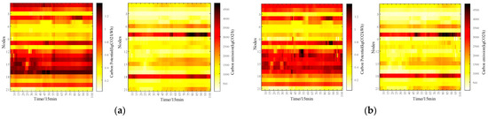
Figure 5.
Carbon potential and carbon emissions at nodes of a provincial-level system on a typical day: (a) Case 1; (b) Case 2.
From the carbon potential and emissions of each node, it is evident that the system’s carbon emissions trend is consistent with the load electricity consumption. With the introduction of renewable energy, the carbon potential and emissions of each node have decreased. It is particularly noteworthy that the carbon emissions of nodes 6, 8, 18, and 21 at each moment are significantly higher than those of other nodes. Combined with Figure A4d, it is known that the load levels of nodes 6, 8, 18, and 21 are significantly higher than those of other nodes, resulting in significantly higher carbon emissions attributed to the load side. To verify the correlation between the carbon potential of each node and the composition of the power generation sources of the node, a detailed analysis of the output of various types of power sources under each node at 14:00 is conducted, as shown in Figure 6.
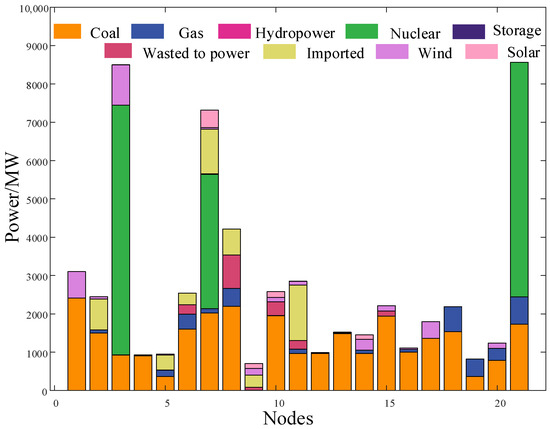
Figure 6.
Distribution of power output across all nodes at 14:00.
Figure 7 shows that nodes 1 and 17 have significantly reduced carbon potential after the introduction of renewable energy due to their high proportion of renewable energy output. However, since the load of these two nodes is relatively low, the reduction in carbon emissions is not significant. In addition, nodes 3, 7, and 21 are connected to nuclear power units. During production operation, the output proportion of nuclear power is high, and the carbon emission factor of nuclear power is much lower than that of coal-fired and gas-fired power. Therefore, the carbon emissions of these three nodes are always lower than those of other nodes with equivalent loads. Further sorting out the comparison of the hourly carbon emission curves of each node under the two scenarios is shown in Figure 7.

Figure 7.
Comparison of carbon emissions in the provincial-level system on a typical day.
Comparing the carbon emissions of each node at each moment, it can be seen that node 3, with a renewable energy proportion of 61.75%, has significantly lower carbon emissions than other nodes. Node 7 sees a significant increase in photovoltaic output in the morning, resulting in a clear downward trend in its carbon emissions. A detailed breakdown of the carbon emissions and energy composition of each node is further shown in Table 6.
Through the comparative analysis of carbon emissions in the provincial system under scenarios with and without renewable energy, it is observed that the output of gas-fired power significantly decreases under the scenario with renewable energy. However, since the proportion of gas-fired power output is small and the carbon emission factor of gas-fired power units is 0.3789, the degree of reduction in carbon emissions per unit is only 3.06% when the proportion of renewable energy is 6.10%.
4.2.3. Analysis of the Rationality of Carbon Emissions Calculated on the Load Side
To analyze the correlation between the proportion of renewable energy output at each node and the degree of reduction in carbon potential, the relationship between the proportion of renewable energy output at each node and the degree of reduction in carbon emissions is organized, as shown in Figure 8.

Figure 8.
Correlation between renewable energy penetration rate and carbon emissions at each Node.
From Figure 8, it can be seen that the degree of carbon emissions reduction in various nodes is generally positively correlated with the proportion of renewable energy. However, due to the existence of branch links between cities, carbon emissions are influenced by adjacent cities.
Taking Node 3 as an example, although it has a high proportion of renewable energy, the degree of carbon emission reduction calculated from the source side is relatively low. This is because some of the renewable energy is provided to the adjacent Node 4, which significantly reduces the degree of carbon emission reduction at Node 4.
A further comparison of the carbon emissions of system nodes calculated from the source side and the load side is shown in Figure 9.
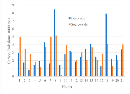
Figure 9.
Comparison of carbon emissions from source side and load side at each node.
Figure 9 shows that the traditional method of calculating carbon emissions from the power supply side is related to the power source structure, while the calculation of carbon emissions from the load side is related to the node carbon potential during the load electricity consumption phase, which can more accurately reflect the actual carbon emissions of the region.
5. Conclusions
This paper establishes a coordinated optimization operation simulation model for source–grid–load–storage systems with the objective of minimizing system costs. It introduces a power flow calculation method and a dynamic zonal carbon emission calculation method, both based on a linkage matrix and the theory of carbon emission flows. The power flow calculation method replaces traditional nonlinear constraints with linear ones, thereby avoiding the computational burden of invoking Matpower and not only reducing the complexity of model solving but also ensuring the accuracy of model solutions. The dynamic zonal carbon emission calculation method addresses the shortcomings of existing methods, which are too coarse-grained and unable to accurately determine the operational states of multiple units at a node. This method enhances the precision of carbon emission metering and clarifies the improvement effect of renewable energy output on the carbon emissions of adjacent regions. The effectiveness and practicality of the proposed methods are validated through case studies based on the IEEE 14-bus system and actual operational data from a provincial power grid. The results of this paper not only provide theoretical support for the coordinated optimization of power system operation and carbon emission management but also offer significant technical references and practical guidance for the sustainable development of future power systems. Although the methods presented in this paper demonstrate good feasibility and guiding value in practical applications, further validation and optimization are needed under broader system scales and more complex operational conditions. Future research could consider incorporating more practical factors, such as market mechanisms and policy elements, into the model to enhance its adaptability and predictive accuracy.
Author Contributions
Conceptualization, investigation, resources, project administration, funding acquisition, X.H. and S.L.; methodology, software, writing—original draft preparation, K.J.; validation, formal analysis, writing—review and editing, H.L.; data curation, visualization, supervision, Z.L. All authors have read and agreed to the published version of the manuscript.
Funding
This research was funded by the Science and Technology Project of China Southern Power Grid Co., Ltd., “Low-carbon Evaluation and Optimal Planning Technology for Source-Grid-Load-Storage Synergy in New Power Systems Considering Electricity-Carbon Coupling” (grant number: GDKJXM20230374).
Acknowledgments
In this article, we would like to thank interns Jiaxuan Ma and Dongjing Lyu for their contributions to the simulation work.
Conflicts of Interest
Authors Xin Huang and Shuxin Luo are employed by the company Power Grid Planning and Research Center of Guangdong Power Grid Co., Ltd. The remaining authors declare that the research was conducted in the absence of any commercial or financial relationships that could be construed as a potential conflict of interest.
Abbreviations
| Symbol | Description |
| Carbon emission factor of unit k at node i | |
| Power flow from node n to node i | |
| Average carbon potential at node n | |
| System operation cost | |
| System carbon emission cost | |
| Deficiency loss cost | |
| Fixed operation and maintenance (O&M) cost | |
| Unit generation cost | |
| Unit start–stop cost | |
| Demand-side response (DSR) operation cost | |
| Energy storage operation cost | |
| , | Conventional unit and DSR unit capacity O&M cost |
| , | Energy storage unit power and unit capacity O&M cost |
| System main body operation duration | |
| , , | Generation cost coefficient of conventional units |
| Generation power of conventional units at time t | |
| Unit start–stop status | |
| , | Unit capacity start and stop costs at time t |
| , | Unit start and stop actions at time t |
| DSR unit power O&M cost at time t | |
| Adjusted power of DSR at time t | |
| Energy storage unit power cost at time t | |
| Discharge power of energy storage at time t | |
| Charge and discharge efficiency of energy storage | |
| Penalty cost per unit of carbon emission | |
| Penalty cost per unit of power supply deficiency | |
| Power deficiency of load m at node i at time t | |
| Inflow power from node n to node i | |
| Generation power of unit k connected at node i | |
| Adjustable depth of unit k connected at node i | |
| Response power of DSR m connected at node i | |
| Power deficiency of load m connected at node i | |
| Power consumption of load m connected at node i | |
| Outflow power from node i to node n | |
| Abandoned power of renewable energy l connected at node i | |
| System load reserve rate | |
| , | Minimum and maximum technical output levels of units |
| , | Maximum upward and downward ramping capabilities of units |
| , | Minimum continuous on and off times of units |
| Forecast energy factor of renewable energy units | |
| Energy state of energy storage | |
| Credible capacity coefficient of generators | |
| Credible capacity coefficient of energy storage | |
| System generation adequacy coefficient | |
| Remaining energy of energy storage s at time t | |
| Important load quantity at node i | |
| Power supply guarantee coefficient for important loads |
Appendix A
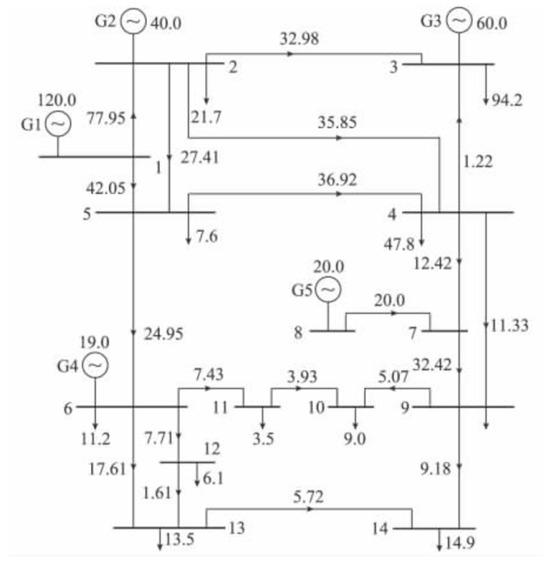
Figure A1.
The steady-state power flow distribution of the IEEE 14-bus system.

Figure A2.
Power flow comparison of IEEE 14- bus system.
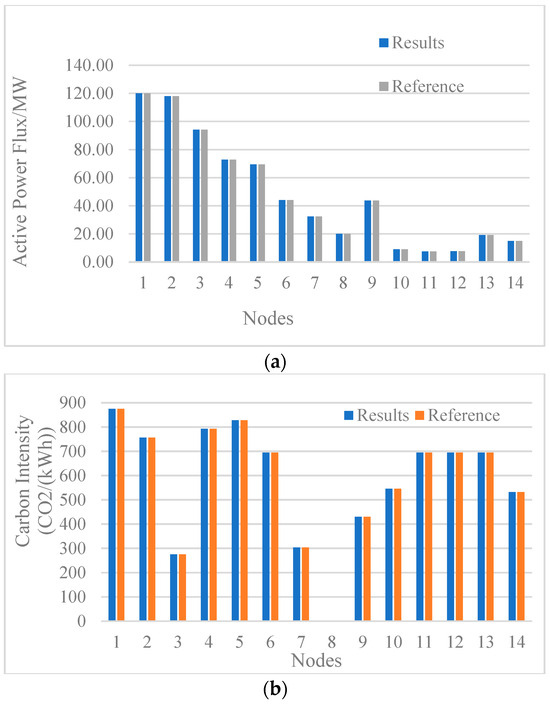
Figure A3.
Nodal active power flux and nodal carbon intensity of IEEE 14-bus system: (a) comparison of active power flux; (b) comparison of carbon intensity.
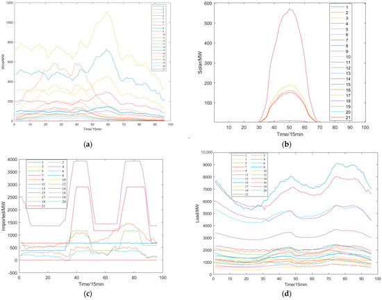
Figure A4.
The relevant boundary curves of the provincial-level system: (a) Typical Daily Wind Power Output Curve; (b) Typical Daily Solar Power Output Curve; (c) Typical Daily Imported Electricity Curve; (d) Typical Daily Load Curve.
Table A1.
Installed capacity of various types of power sources in the 21-node system. Unit: MW.
Table A1.
Installed capacity of various types of power sources in the 21-node system. Unit: MW.
| Node | Coal-Fired Powe | Gas-Fired Powe | Energy Storage | Photovoltaic | Pumped Storage | Hydropower | Offshore Wind Power | Nuclear Power |
|---|---|---|---|---|---|---|---|---|
| 1 | 4580 | 10 | 2.4 | 1201.5 | ||||
| 2 | 3130 | |||||||
| 3 | 5000 | 1200 | 3500 | 6516 | ||||
| 4 | 1140 | 15.23 | ||||||
| 5 | 700 | 1712 | ||||||
| 6 | 2900 | 1340.8 | 2.5 | |||||
| 7 | 6020 | 906 | 778 | 3500 | ||||
| 8 | 3680 | 4276.6 | 2400 | |||||
| 9 | 1003.2 | 220 | 1280 | 266 | ||||
| 10 | 3860 | 257.8 | 132 | |||||
| 11 | 2660 | 2550 | 2400 | 250 | ||||
| 12 | 3200 | 515 | ||||||
| 13 | 2790 | 1200 | 144 | |||||
| 14 | 3200 | 207.64 | 824.5 | |||||
| 15 | 5272 | 245 | ||||||
| 16 | 3260 | |||||||
| 17 | 4520 | 1400 | ||||||
| 18 | 2640 | 5071.4 | 10 | |||||
| 19 | 600 | 4618 | ||||||
| 20 | 2600 | 2990 | 370.75 | |||||
| 21 | 4060 | 3097.6 | 1200 | 6120 |
Table A2.
Installed capacity of gas-fired power units at each node of the 21-node system. Unit: MW.
Table A2.
Installed capacity of gas-fired power units at each node of the 21-node system. Unit: MW.
| Node | 5 | 6 | 7 | 8 | 9 | 11 | 18 | 19 | 20 | 21 | |
|---|---|---|---|---|---|---|---|---|---|---|---|
| Unit | |||||||||||
| 1 | 304 | 329.9 | 303 | 441 | 336.6 | 390 | 475 | 390 | 465 | 390 | |
| 2 | 304 | 329.9 | 303 | 441 | 336.6 | 390 | 475 | 390 | 465 | 390 | |
| 3 | 273 | 160.5 | 150 | 423 | 165 | 390 | 336.6 | 340 | 320 | 390 | |
| 4 | 273 | 160.5 | 150 | 423 | 165 | 310 | 336.6 | 340 | 320 | 390 | |
| 5 | 143 | 120 | 0 | 390 | 0 | 310 | 336.6 | 340 | 270 | 390 | |
| 6 | 143 | 120 | 0 | 390 | 0 | 310 | 336.6 | 320 | 270 | 390 | |
| 7 | 136 | 60 | 0 | 320 | 0 | 150 | 326.85 | 320 | 140 | 336.6 | |
| 8 | 136 | 60 | 0 | 320 | 0 | 150 | 326.85 | 320 | 140 | 180 | |
| 9 | 0 | 0 | 0 | 228.3 | 0 | 150 | 325 | 181 | 120 | 161 | |
| 10 | 0 | 0 | 0 | 228.3 | 0 | 0 | 325 | 181 | 120 | 80 | |
| 11 | 0 | 0 | 0 | 140 | 0 | 0 | 165 | 140 | 120 | 0 | |
| 12 | 0 | 0 | 0 | 140 | 0 | 0 | 160 | 140 | 120 | 0 | |
| 13 | 0 | 0 | 0 | 136 | 0 | 0 | 150 | 140 | 60 | 0 | |
| 14 | 0 | 0 | 0 | 136 | 0 | 0 | 145.65 | 120 | 60 | 0 | |
| 15 | 0 | 0 | 0 | 60 | 0 | 0 | 145.65 | 120 | 0 | 0 | |
| 16 | 0 | 0 | 0 | 60 | 0 | 0 | 145 | 120 | 0 | 0 | |
| 17 | 0 | 0 | 0 | 0 | 0 | 0 | 145 | 120 | 0 | 0 | |
| 18 | 0 | 0 | 0 | 0 | 0 | 0 | 120 | 120 | 0 | 0 | |
| 19 | 0 | 0 | 0 | 0 | 0 | 0 | 120 | 120 | 0 | 0 | |
| 20 | 0 | 0 | 0 | 0 | 0 | 0 | 60 | 88 | 0 | 0 | |
| 21 | 0 | 0 | 0 | 0 | 0 | 0 | 60 | 88 | 0 | 0 | |
| 22 | 0 | 0 | 0 | 0 | 0 | 0 | 55 | 60 | 0 | 0 | |
| 23 | 0 | 0 | 0 | 0 | 0 | 0 | 0 | 60 | 0 | 0 | |
| 24 | 0 | 0 | 0 | 0 | 0 | 0 | 0 | 60 | 0 | 0 | |
Table A3.
Installed capacity of coal-fired power units at each node of the 21-node system. Unit: MW.
Table A3.
Installed capacity of coal-fired power units at each node of the 21-node system. Unit: MW.
| Node | 1 | 2 | 3 | 4 | 5 | 6 | 7 | 8 | 9 | 10 | 11 | 12 | 13 | 14 | 15 | 16 | 17 | 18 | 19 | 20 | 21 | |
|---|---|---|---|---|---|---|---|---|---|---|---|---|---|---|---|---|---|---|---|---|---|---|
| Unit | ||||||||||||||||||||||
| 1 | 1000 | 1000 | 1240 | 300 | 350 | 600 | 1000 | 330 | 0 | 600 | 1000 | 1000 | 600 | 1000 | 1036 | 1000 | 1000 | 660 | 300 | 700 | 1050 | |
| 2 | 1000 | 1000 | 1240 | 300 | 350 | 600 | 1000 | 330 | 0 | 600 | 1000 | 1000 | 600 | 1000 | 1036 | 1000 | 1000 | 660 | 300 | 700 | 1050 | |
| 3 | 600 | 600 | 660 | 135 | 0 | 330 | 150 | 330 | 0 | 350 | 330 | 600 | 300 | 600 | 1000 | 630 | 660 | 660 | 0 | 600 | 330 | |
| 4 | 600 | 330 | 660 | 135 | 0 | 330 | 150 | 330 | 0 | 350 | 330 | 600 | 300 | 600 | 1000 | 600 | 660 | 330 | 0 | 600 | 330 | |
| 5 | 330 | 200 | 600 | 135 | 0 | 320 | 600 | 330 | 0 | 350 | 0 | 0 | 300 | 0 | 600 | 30 | 600 | 330 | 0 | 0 | 330 | |
| 6 | 330 | 0 | 600 | 135 | 0 | 320 | 630 | 330 | 0 | 350 | 0 | 0 | 300 | 0 | 300 | 0 | 600 | 0 | 0 | 0 | 330 | |
| 7 | 330 | 0 | 0 | 0 | 0 | 200 | 630 | 320 | 0 | 330 | 0 | 0 | 135 | 0 | 300 | 0 | 0 | 0 | 0 | 0 | 320 | |
| 8 | 330 | 0 | 0 | 0 | 0 | 200 | 630 | 320 | 0 | 330 | 0 | 0 | 135 | 0 | 0 | 0 | 0 | 0 | 0 | 0 | 320 | |
| 9 | 30 | 0 | 0 | 0 | 0 | 0 | 600 | 320 | 0 | 300 | 0 | 0 | 60 | 0 | 0 | 0 | 0 | 0 | 0 | 0 | 0 | |
| 10 | 30 | 0 | 0 | 0 | 0 | 0 | 630 | 320 | 0 | 300 | 0 | 0 | 60 | 0 | 0 | 0 | 0 | 0 | 0 | 0 | 0 | |
| 11 | 0 | 0 | 0 | 0 | 0 | 0 | 0 | 210 | 0 | 0 | 0 | 0 | 0 | 0 | 0 | 0 | 0 | 0 | 0 | 0 | 0 | |
| 12 | 0 | 0 | 0 | 0 | 0 | 0 | 0 | 210 | 0 | 0 | 0 | 0 | 0 | 0 | 0 | 0 | 0 | 0 | 0 | 0 | 0 | |
References
- Masson-Delmotte, V.; Zhai, P.; Pörtner, H.O.; Roberts, D.; Skea, J.; Shukla, P.R. An IPCC Special Report on the Impacts of Global Warming of 1.5 C Above Pre-Industrial Levels and Related Global Greenhouse Gas Emission Pathways, in the Context of Strengthening the Global Response to the Threat of Climate Change, Sustainable Development, and Efforts to Eradicate Poverty; Cambridge University Press: Cambridge, UK; New York, NY, USA, 2018; pp. 3–24. [Google Scholar] [CrossRef]
- State Grid Energy Research Institute Co., Ltd. China Energy & Electricity Outlook; China Electricity Power Press: Beijing, China, 2021. [Google Scholar]
- National Energy Administration. National Power Industry Statistics in 2023. Available online: https://www.nea.gov.cn/2024-01/26/c_1310762246.htm (accessed on 26 January 2024).
- China Electricity Council. Annual Development Report of China Power Industry. 2023. Available online: https://www.cec.org.cn/detail/index.html?3-322625 (accessed on 30 January 2024).
- Zhang, Z.; Kang, C. Challenges and prospects for constructing the new-type system towards a carbon neutrality power future. Proc. CESS 2022, 42, 2806–2818. [Google Scholar] [CrossRef]
- Chen, Y.; Jing, L.; Ye, P.; Deng, S.; Han, Z. Research on Low-Carbon Assessment and Carbon Reduction Measures for New Distribution Network. Northeast Electr. Power Technol. 2024, 45, 26–31+35. [Google Scholar]
- Xu, Q. Discussion on Carbon Accounting of Steam Boilers based on Emission Factor Method. Ind. Boil. 2023, 4, 12–15+35. [Google Scholar] [CrossRef]
- Ran, P.; Wang, J.; Li, Z.; Liu, X.; Zeng, Q.; Li, W. General Matrix Model of Carbon Emissions and Carbon Sensitivity of Thermal Power Units. J. Chin. Soc. Power Eng. 2024, 44, 947–955. [Google Scholar] [CrossRef]
- Yao, S.; Zhi, J.; Fu, J.; Li, Z.; Lu, Z.; Zhuo, J. Research Progress of Online Carbon Emission Monitoring Technology for Thermal Power Enterprises. J. South China Univ. Technol. (Nat. Sci. Ed.) 2023, 51, 97–108. [Google Scholar] [CrossRef]
- Xu, X.; Ji, X.; Wang, H. Research on Optimization of Combined Cooling, Heating and Power System Based on Full Life Cycle Evaluation. Acta Energiae Solaris Sin. 2024, 45, 360–368. [Google Scholar] [CrossRef]
- Liu, Y.; Li, Y.; Zhou, C.; Song, J.; Deng, H.; Du, E.; Zhang, N.; Kang, C. A Review of Carbon Emission Measurement and Analysis Methods in Power Systems. Proc. Chin. Soc. Electr. Eng. 2024, 44, 2220–2236. [Google Scholar] [CrossRef]
- Kang, C.; Du, E.; Li, Y.; Zhang, N.; Chen, Q.; Guo, H.; Wang, P. Key Scientific Problems and Research Framework for Carbon Perspective Research of New Power Systems. Power Syst. Technol. 2022, 46, 821–833. [Google Scholar] [CrossRef]
- Zhang, N.; Li, Y.; Huang, J.; Li, Y.; Du, E.; Li, M.; Liu, Y.; Kang, C. Carbon Measurement Method and Carbon Meter System for Whole Chain of Power System. Autom. Electr. Power Syst. 2023, 47, 2–12. [Google Scholar]
- Zhou, T.; Kang, C.; Xu, Q.; Chen, Q. Preliminary theoretical investigation on power system carbon emission flow. Autom. Electr. Power Syst. 2012, 36, 38–43+85. [Google Scholar] [CrossRef]
- Ou, Z.; Yang, K.; Lou, Y.; Peng, S.; Li, P.; Zhou, Q. Consider Carbon Emission Flow Analysis of Power System with Regards to Power Loss and Wind Power Uncertainty. J. Phys. Conf. Ser. 2023, 2584, 012107. [Google Scholar] [CrossRef]
- Zhou, T.; Kang, C.; Xu, Q.; Chen, Q. Preliminary investigation on a method for carbon emission flow calculation of power system. Autom. Electr. Power Syst. 2012, 36, 44–49. [Google Scholar] [CrossRef]
- Zheng, C.; Zhang, X.; Su, L.; Gao, H.; Xiao, X.; Zhang, L.; Qi, Y. Low-carbon economic operation control strategy of integrated energy system under carbon emission trading mechanism. Electr. Eng. 2023, 14, 10–15+20. [Google Scholar] [CrossRef]
- Wang, J.; Qiu, Z.; Zhang, X.; Dou, M.; Liu, X.; Lu, Y.; Lv, X.; Wang, L. Operation optimization strategy of distribution area considering renewable energy output uncertainty and carbon emission cost. Renew. Energy 2024, 42, 407–419. [Google Scholar] [CrossRef]
- Zhang, S.; Li, Y.; Liu, W.; Sun, S.; Yu, P.; Zhang, N. Multi-objective optimization allocation method for cloud energy storage in microgrid clusters considering economy, low carbon, and reliability. Autom. Electr. Power Syst. 2024, 48, 21–30. [Google Scholar] [CrossRef]
- Liu, Y.; Yao, L.; Zhao, B.; Xu, J.; Liao, S.; Pang, X. Low-carbon economic dispatch method for distribution network-microgrid cluster considering flexible grouping. Autom. Electr. Power Syst. 2024, 1–23. [Google Scholar] [CrossRef]
- Motalleb, M.; Reihani, E.; Ghorbani, R. Optimal placement and sizing of the storage supporting transmission and distribution networks. Renew. Energy 2016, 94, 651–659. [Google Scholar] [CrossRef]
- Wang, C.; Chen, Y.; Chi, C.; Tao, Y.; Li, X.; Jiang, X. Calculation Method of Power System Carbon Emission Flow Based on Power Flow Distribution Matrix. Sci. Technol. Eng. 2022, 22, 4835–4842. [Google Scholar]
- Zhao, J.; Ye, J.; Deng, Y. Comparative analysis on DC power flow and AC power flow. Power Syst. Technol. 2012, 36, 147–152. [Google Scholar]
- Zhu, J.; Shi, K.; Li, Q.; Yu, R.Y.; Xia, J.R.; Yuan, Y. Time series production simulation and renewable energy accommodation capacity evaluation considering transmission network power flow constraints. Power Syst. Technol. 2022, 46, 1947–1955. [Google Scholar] [CrossRef]
- Bo, L. Research on New Power System Optimization Planning Method Considering Operation Simulation under Low Carbon Targets. Ph.D. Thesis, Chongqing University, Chongqing, China, 2022. [Google Scholar]
- Liu, R.; Bao, Z.; Lin, Z. Distributed Low-Carbon Economic Dispatching Coordination of Source, Grid and Load Considering Dual Layer Ladder-Type Carbon Price Mechanism with Reward and Punishment. Autom. Electr. Power Syst. 2024, 9, 11–20. [Google Scholar]
- Cui, Y.; Jiang, S.; Zhao, Y.; Xu, Y.; Zhang, J.; Wang, M.; Wang, Z. Comprehensive energy system low-carbon optimization dispatch considering ultra-carbon demand response. Power Syst. Technol. 2024, 48, 1863–1872. [Google Scholar] [CrossRef]
- Liu, K.; Li, L.; Lin, Z.; Zhao, Q.; Yang, F.; Wang, X. Low-carbon economic dispatch of electricity-gas interconnected system considering carbon emission flow. Electr. Power Autom. Equip. 2024, 44, 1–10. [Google Scholar] [CrossRef]
- Qiao, W.; Han, Y.; Si, F.; Li, K.; Wang, J.; Zhao, Q. Optimal Economic-Emission Scheduling of Coupled Transportation and Power Distribution Networks with Multi-Objective Optimization. IEEE Trans. Ind. Appl. 2023, 59, 4808–4820. [Google Scholar] [CrossRef]
- Ma, M.; Li, Y.; Du, E.; Jiang, H.; Zhang, N.; Wang, W.; Wang, M. Calculating Probabilistic Carbon Emission Flow: An Adaptive Regression-Based Framework. IEEE Trans. Sustain. Energy 2024, 15, 1576–1588. [Google Scholar] [CrossRef]
- Zhang, J.; Sun, J.; Wu, C. Enable a Carbon Efficient Power Grid via Minimal Uplift Payments. IEEE Trans. Sustain. Energy 2022, 13, 1329–1343. [Google Scholar] [CrossRef]
- Yang, Y.; Qiu, J.; Zhang, C. Distribution Network Planning Towards a Low-Carbon Transition: A Spatial-Temporal Carbon Response Method. IEEE Trans. Sustain. Energy 2024, 15, 429–442. [Google Scholar] [CrossRef]
- Zhang, J.; Sang, L.; Xu, Y.; Sun, H. Networked Multiagent-Based Safe Reinforcement Learning for Low-Carbon Demand Management in Distribution Networks. IEEE Trans. Sustain. Energy 2024, 15, 1528–15452024. [Google Scholar] [CrossRef]
- Radovanović, A.; Koningstein, R.; Schneider, I.; Chen, B.; Duarte, A.; Roy, B.; Xiao, D.; Haridasan, M.; Hung, P.; Care, N.; et al. Carbon-Aware Computing for Datacenters. IEEE Trans. Power Syst. 2023, 38, 1270–1280. [Google Scholar] [CrossRef]
- Wang, Y.; Qiu, J.; Tao, Y. Optimal Power Scheduling Using Data-Driven Carbon Emission Flow Modelling for Carbon Intensity Control. IEEE Trans. Power Syst. 2022, 37, 2894–2905. [Google Scholar] [CrossRef]
- Yang, L.; Luo, J.; Xu, Y.; Zhang, Z.; Dong, Z. A Distributed Dual Consensus ADMM Based on Partition for DC-DOPF with Carbon Emission Trading. IEEE Trans. Ind. Inform. 2020, 16, 1858–1872. [Google Scholar] [CrossRef]
- Akbari-Dibavar, A.; Mohammadi-Ivatloo, B.; Zare, K.; Khalili, T.; Bidram, A. Economic-Emission Dispatch Problem in Power Systems with Carbon Capture Power Plants. IEEE Trans. Ind. Appl. 2021, 57, 3341–3351. [Google Scholar] [CrossRef]
- Li, J.; Zou, N.; Wu, J.; Yang, Q. Low carbon optimal dispatching of power system considering carbon emission flow theory. In Proceedings of the 2022 9th International Forum on Electrical Engineering and Automation (IFEEA), Zhuhai, China, 4–6 November 2022; pp. 532–536. [Google Scholar] [CrossRef]
- Yang, Y.; Liu, J.; Xu, X.; Xie, K. Two-Stage Low-Carbon Optimal Scheduling of Power System Based on Carbon Flow Theory and Demand Response. In Proceedings of the 2023 Panda Forum on Power and Energy (PandaFPE), Chengdu, China, 27–30 April 2023; pp. 1030–1034. [Google Scholar] [CrossRef]
- Zhang, L.; Zeng, L.; Wu, H.; Liu, H.; Liao, P.; Chen, Y. Optimal Scheduling of Load Aggregators Participating in Demand Response Market under Low-Carbon Power System. In Proceedings of the 2021 IEEE 5th Conference on Energy Internet and Energy System Integration (EI2), Taiyuan, China, 22–24 October 2021; pp. 4034–4040. [Google Scholar] [CrossRef]
- Li, Y.; Liu, Y.; Yang, X.; He, W.; Fang, Y.; Du, E.; Zhang, N.; Li, J. Electricity Carbon Metering Method Considering Electricity Transaction Information. Proc. Chin. Soc. Electr. Eng. 2024, 44, 439–451. [Google Scholar] [CrossRef]
- Jacobson, M.Z. 100% Clean, Renewable Energy and Storage for Everything; Cambridge University Press: Cambridge, UK, 2020. [Google Scholar]
- Li, M.; Fan, Y.; Wang, Y.; Wang, W.; Niu, S.; Wei, W. Coordinated optimization of wind and solar power storage in new energy bases. Electr. Power Autom. Equip. 2024, 44, 18. [Google Scholar] [CrossRef]
- Li, B.; Chen, M.; Zhong, H.; Ma, Z.; Liu, D.; He, G. A Review of Long-term Planning of New Power Systems with Large Share of Renewable Energy. Proc. Chin. Soc. Electr. Eng. 2023, 43, 555–581. [Google Scholar] [CrossRef]
- Ding, K.; Sun, Y.; Wang, X.; Yang, C.; Li, H. Configuration method of concentrating solar power plant in renewable energy base considering confidence capacity and peak shaving capacity. Guangdong Electr. Power 2024, 37, 25–34. [Google Scholar] [CrossRef]
- Denholm, P.; Nunemaker, J.; Gagnon, P.; Cole, W. The potential for battery energy storage to provide peaking capacity in the United States. Renew. Energy 2020, 151, 1269–1277. [Google Scholar] [CrossRef]
Disclaimer/Publisher’s Note: The statements, opinions and data contained in all publications are solely those of the individual author(s) and contributor(s) and not of MDPI and/or the editor(s). MDPI and/or the editor(s) disclaim responsibility for any injury to people or property resulting from any ideas, methods, instructions or products referred to in the content. |
© 2024 by the authors. Licensee MDPI, Basel, Switzerland. This article is an open access article distributed under the terms and conditions of the Creative Commons Attribution (CC BY) license (https://creativecommons.org/licenses/by/4.0/).