

Assessing the Outcomes of Digital Transformation Smartization Projects in Industrial Enterprises: A Model for Enabling Sustainability

 ,
,
Abstract
:1. Introduction
- –
- To study the essence of the concept of smartization and digital transformation smartization projects;
- –
- To explore the relationship between smartization and sustainable development;
- –
- To develop a system of indicators for evaluating the results of the implementation of DTSP;
- –
- To develop a model for diagnosing the results of implementing DTSP for industrial enterprise;
- –
- To test the proposed model on a sample of industrial enterprises.
2. Theoretical Framework
2.1. The Concept of Smartization and Digital Transformation Smartization Projects
2.2. Linking Smartization and Sustainable Development
- Resource Optimization: At the core of smartization lies the ability to optimize resource utilization [9]. Through real-time data analytics and process automation, industrial enterprises can reduce energy consumption, minimize waste, and enhance resource efficiency. This not only lowers operational costs but also reduces the enterprise’s ecological footprint;
- Emissions Reduction: Smartization empowers industrial enterprises to monitor and control emissions more effectively. Whether through predictive maintenance to reduce emissions from machinery or by optimizing logistics to minimize transportation-related emissions, digital technologies play a pivotal role in advancing sustainability [10,11];
- Circular Economy Integration: Smartization projects enable the transition to a circular economy model, where products and materials are reused, refurbished, or recycled. By tracking product lifecycles, managing returns efficiently, and promoting sustainable product design, enterprises can contribute to a more circular and environmentally responsible economy [12,13];
- Supply Chain Transparency: Digital transformation enhances transparency within the supply chain. This transparency is essential for identifying and mitigating social and environmental risks in the supply network, ensuring suppliers adhere to sustainable practices [16];
- Social Responsibility: Sustainable development extends beyond environmental concerns to encompass social responsibility [17]. Smartization projects can include initiatives to improve workplace safety, labor conditions, and employee well-being, contributing to the social pillar of sustainability;
- Stakeholder Engagement: Smartization facilitates better engagement with stakeholders, including customers, investors, and the community. Demonstrating a commitment to sustainability through digital transparency and reporting can enhance an enterprise’s reputation and build trust;
- Long-Term Resilience: By optimizing operations and reducing environmental risks, smartization projects enhance an enterprise’s long-term resilience in the face of climate change, resource scarcity, and other sustainability-related challenges;
- Data-Driven Decision-Making: Smartization leverages data analytics to inform decision-making. This data-driven approach allows enterprises to make informed choices that align with their sustainability objectives, from supply chain optimization to energy management.
2.3. Development of Indicators for Diagnosing the Results of the Implementation of DTSP for Industrial Enterprises
2.4. Economic Evaluation of the Implementation of Diagnosed DTSP for Enterprises
3. Research Method
4. Results
- (1)
- For each indicator from the selected sets, the structure and dynamics of changes during the calendar year 2021 are monitored, and attention is paid to the smoothness of changes in indicators and the connections between them;
- (2)
- As far as possible, the influence of price indexation, exchange rate fluctuations, and the influence of state regulation is eliminated;
- (3)
- A dynamic model of indicator increments is formed, i.e., the trends of changes in each indicator are monitored in the absence of additional influences;
- (4)
- The hypothetical impacts of the smartization project are superimposed on each indicator (in proportion to those that actually occurred at PJSC “Odeskabel” and PJSC “LLRP”);
- (5)
- Parameter differences are monitored, and the “net” impact of the diagnosed smartization project is calculated.
5. Discussion and Conclusions
- –
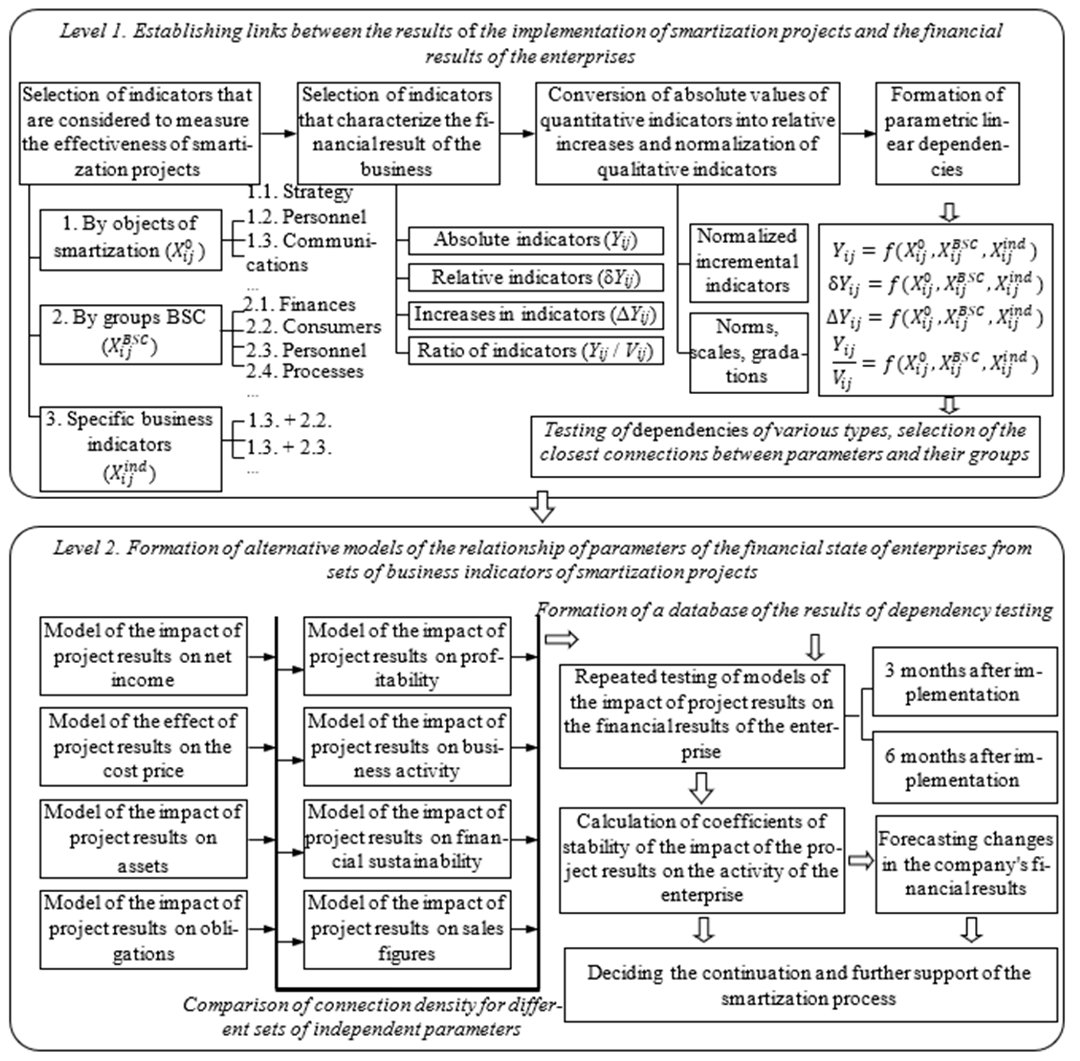
- A two-level graphical and analytical model for diagnosing the results of the implementation of DTSP (Figure 2), which allows for taking into account the interests of the project participants regarding the choice of diagnosis methods and techniques for identifying alternative sets of business indicators for each object of influence of the smartization project, to establish economic and non-economic criteria for evaluating the effectiveness of consulting, as well as perform monitoring of indicators and automated processing of diagnostic results to regulate deviations from the optimal values of project results. At the first level, sustainable relationships between the project effectiveness parameters of DTSP and the financial results of the customer enterprise are identified and described. At the second stage of the economic evaluation of the implementation of diagnosed DTSP, alternative models of the relationship of key parameters of enterprises’ financial state with sets of DTSP results are formed either by objects of influence or by crucial business indicators with a universal purpose. Conducted research and calculations show that in most cases, the density of communication between parameters is not high; therefore, it is advisable to form an economic–mathematical model for optimizing the implementation of diagnosed DTSP, which will be able to reconcile the costs of implementing the project solutions with the requirements for minimizing deviations of the actual values of business indicators from the planned and at the same time ensure the slightest possible disturbances in the rhythm of production. The formed economic–mathematical model contains three equivalent functions of the goal: F1(x)—minimization of uncovered costs for the design, implementation and maintenance of the smartization project; F2(y)—minimization of negative deviations of the actual values of business indicators from the planned ones; F3(z)—depreciation of violations production rhythms in the process of implementing the smartization project, which in the general formulation of the problem have the same significance; therefore we can use the scheme of uniform optimization. This model can be used at any stage of the smartization project. Based on it, conclusions can be drawn regarding the effectiveness of the implementation of the entire project and its individual stages, objects, or elements. The advantage of this model is the possibility of its decomposition, that is, a division into separate parts with the possibility of introducing additional restrictions or, conversely, reducing the level of requirements for some of them;
- –
- A matrix for selecting indicators for diagnosing the results of the implementation of DTSP for industrial enterprises (Table 2), which showed its effectiveness when tested at industrial enterprises;
- –
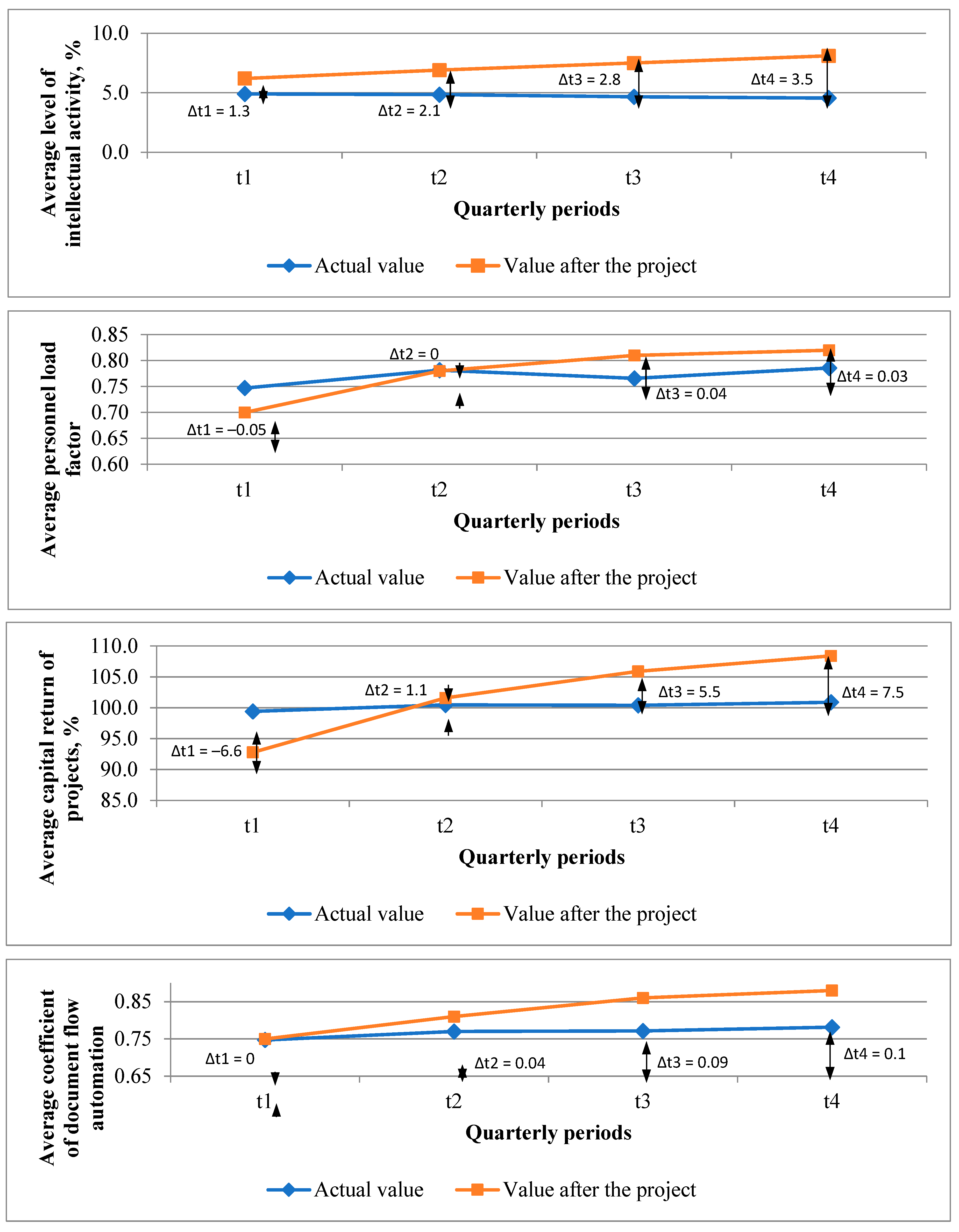
- Simulation modeling of the impact of a smartization project on the performance of industrial enterprises was carried out (based on the hypothesis that these enterprises will develop stably even without smartization within the limits of the increases in indicators that they demonstrated in previous periods). The influence of external environmental factors is excluded, and the deviations in demand, prices, exchange rates, and the consequences of state regulation are neglected. In such conditions, a computer simulation was carried out, which involved reproducing the impact of real DTSP of PJSC “Odeskabel” and PJSC “LLRP” on the input data of the other five enterprises in the same time intervals.
6. Limitations of this Study
- –
- Definition of smartization as a process in its essence;
- –
- Management of the smartization process is defined as a project management process, that is, one that has a clear time frame, resources, executors, etc.;
- –
- The smartization project is carried out by a third-party organization (not by the enterprise itself) for an industrial enterprise.
Author Contributions
Funding
Institutional Review Board Statement
Informed Consent Statement
Data Availability Statement
Conflicts of Interest
Appendix A

| Enterprises | The Value of Indicators | |||||||||||||||
|---|---|---|---|---|---|---|---|---|---|---|---|---|---|---|---|---|
| Balance Sheet Assets | Non-Current Assets | Intangible Assets | Current Asset | |||||||||||||
| t1 | t2 | t3 | t4 | t1 | t2 | t3 | t4 | t1 | t2 | t3 | t4 | t1 | t2 | t3 | t4 | |
| PJSC “LLRP” | 245,002 | 247,574 | 247,968 | 268,576 | 131,864 | 131,500 | 130,340 | 134,035 | 4312 | 4357 | 4488 | 4740 | 113,138 | 116,074 | 117,628 | 134,541 |
| PJSC “Odeskabel” | 1,093,358 | 1,109,748 | 1,108,564 | 1,117,976 | 139,584 | 141,252 | 144,281 | 144,885 | 13,978 | 14,520 | 15,218 | 15,332 | 953,774 | 968,496 | 964,283 | 973,091 |
| PJSC “Iskra” | 21,444,785 | 23,528,546 | 25,235,330 | 25,245,657 | 6,066,133 | 6,142,107 | 6,288,825 | 6,852,489 | 1800 | 1782 | 5705 | 5266 | 15,378,652 | 17,386,439 | 18,946,505 | 18,393,168 |
| PJSC “Azot” | 419,589 | 422,159 | 431,580 | 434,835 | 79,859 | 78,443 | 80,564 | 80,229 | 785 | 748 | 756 | 762 | 339,730 | 343,716 | 351,016 | 354,606 |
| PJSC “Radar” | 518,966 | 497,832 | 528,238 | 530,632 | 312,197 | 311,966 | 311,813 | 333,823 | 215,829 | 215,843 | 215,894 | 240,025 | 206,769 | 185,866 | 216,425 | 196,809 |
| JSC “Ekvator” | 337,973 | 336,390 | 332,448 | 329,975 | 300,954 | 300,745 | 300,912 | 309,999 | 1392 | 1392 | 1253 | 1253 | 37,019 | 35,645 | 31,536 | 19,976 |
| PJSC “KBVP” | 1,068,497 | 1,066,798 | 1,069,577 | 1,069,979 | 924,458 | 924,980 | 925,948 | 927,017 | 1200 | 1236 | 1249 | 1199 | 144,039 | 141,818 | 143,629 | 142,962 |
| Enterprises | The Value of Indicators | |||||||||||||||
|---|---|---|---|---|---|---|---|---|---|---|---|---|---|---|---|---|
| Balance Sheet liabilities | Own Capital | Long-Term Liabilities | Current Liabilities | |||||||||||||
| t1 | t2 | t3 | t4 | t1 | t2 | t3 | t4 | t1 | t2 | t3 | t4 | t1 | t2 | t3 | t4 | |
| PJSC “LLRP” | 245,002 | 247,574 | 247,968 | 268,576 | 153,283 | 141,103 | 132,795 | 131,230 | 826 | 670 | 662 | 393 | 90,893 | 105,801 | 114,511 | 136,953 |
| PJSC “Odeskabel” | 1,093,358 | 1,109,748 | 1,108,564 | 1,117,976 | −294,938 | −297,955 | −285,970 | −273,887 | 111,068 | 113,189 | 113,189 | 116,781 | 1,277,228 | 1,294,514 | 1,281,345 | 1,275,082 |
| PJSC “Iskra” | 21,444,785 | 23,528,546 | 25,235,330 | 25,245,657 | 14,128,146 | 15,517,954 | 16,500,510 | 16,342,312 | 1,257,610 | 4,199,314 | 4,176,924 | 3,376,012 | 6,059,029 | 3,811,278 | 4,557,896 | 5,527,333 |
| PJSC “Azot” | 419,589 | 422,159 | 431,580 | 434,835 | 324,205 | 324,205 | 324,205 | 324,205 | 786 | 759 | 795 | 771 | 94,598 | 97,195 | 106,580 | 109,859 |
| PJSC “Radar” | 518,966 | 497,832 | 528,238 | 530,632 | 414,570 | 405,708 | 428,102 | 452,871 | 681 | 692 | 692 | 637 | 103,715 | 91,432 | 99,444 | 77,124 |
| JSC “Ekvator” | 337,973 | 336,390 | 332,448 | 329,975 | 304,453 | 293,214 | 290,549 | 290,090 | 415 | 1605 | 1800 | 1992 | 33,105 | 41,571 | 40,099 | 37,893 |
| PJSC “KBVP” | 1,068,497 | 1,066,798 | 1,069,577 | 1,069,979 | −415,928 | −428,458 | −436,190 | −447,158 | 205,259 | 204,869 | 206,171 | 207,377 | 1,279,166 | 1,290,387 | 1,299,596 | 1,309,760 |
| Enterprises | The Value of Indicators | |||||||||||||||
|---|---|---|---|---|---|---|---|---|---|---|---|---|---|---|---|---|
| Net Income from Product Sales | Cost of Goods Sold | Gross Profit | Net Profit | |||||||||||||
| t1 | t2 | t3 | t4 | t1 | t2 | t3 | t4 | t1 | t2 | t3 | t4 | t1 | t2 | t3 | t4 | |
| PJSC “LLRP” | 27,356 | 59,413 | 82,628 | 116,924 | 26,425 | 59,522 | 83,638 | 178,490 | 931 | −109 | −1010 | −61,566 | −11,158 | −22,979 | −33,083 | −35,944 |
| PJSC “Odeskabel” | 115,984 | 235,959 | 408,887 | 526,259 | 107,998 | 203,187 | 355,287 | 428,836 | 7986 | 32,772 | 53,600 | 97,423 | −3195 | −10,958 | −16,352 | −20,931 |
| PJSC “Iskra” | 2,111,134 | 5,058,087 | 7,541,346 | 10,496,206 | 747,833 | 1,809,703 | 2,915,451 | 4,220,240 | 1,363,301 | 3,248,384 | 4,625,895 | 6,275,966 | 310,665 | 1,279,660 | 1,860,610 | 1,955,441 |
| PJSC “Azot” | 113,085 | 197,750 | 312,287 | 514,113 | 98,580 | 166,095 | 253,811 | 407,132 | 14,505 | 31,655 | 58,476 | 106,981 | 6618 | 23,098 | 42,610 | 51,504 |
| PJSC “Radar” | 28,690 | 73,445 | 146,267 | 205,106 | 22,450 | 60,493 | 121,056 | 168,047 | 6240 | 12,952 | 25,211 | 37,059 | 896 | 1456 | 18,988 | 21,652 |
| JSC “Ekvator” | 7811 | 14,803 | 21,636 | 29,421 | 5738 | 11,847 | 28,774 | 28,394 | 2073 | 2956 | −7138 | 1027 | −3081 | −10,610 | −12,375 | −13,234 |
| PJSC “KBVP” | 59,852 | 105,787 | 155,190 | 223,545 | 60,198 | 108,284 | 163,457 | 235,873 | −346 | −2497 | −8267 | −12,328 | −599,124 | −613,248 | −694,941 | −666,757 |
| Enterprises | The Value of Indicators | |||||||||||||||
|---|---|---|---|---|---|---|---|---|---|---|---|---|---|---|---|---|
| Administrative Expenses | Sales Expenses | Labor Costs | Deductions for Social Events | |||||||||||||
| t1 | t2 | t3 | t4 | t1 | t2 | t3 | t4 | t1 | t2 | t3 | t4 | t1 | t2 | t3 | t4 | |
| PJSC “LLRP” | 8878 | 16,885 | 24,424 | 33,745 | 226 | 434 | 552 | 833 | 16,669 | 31,765 | 45,332 | 64,402 | 3667 | 6988 | 9973 | 14,168 |
| PJSC “Odeskabel” | 7668 | 15,861 | 23,681 | 30,216 | 5237 | 9668 | 14,580 | 21,236 | 17,945 | 37,985 | 54,510 | 71,688 | 3948 | 8357 | 11,992 | 15,771 |
| PJSC “Iskra” | 248,238 | 508,166 | 752,166 | 1,052,515 | 58,858 | 98,352 | 245,153 | 378,887 | 444,220 | 879,171 | 1,362,583 | 1,835,975 | 97,728 | 193,418 | 299,768 | 403,915 |
| PJSC “Azot” | 10,259 | 21,689 | 30,457 | 41,975 | 3038 | 6648 | 8970 | 12,535 | 33,158 | 65,884 | 95,702 | 132,289 | 7295 | 14,494 | 21,054 | 29,104 |
| PJSC “Radar” | 3457 | 7160 | 11,307 | 15,241 | 724 | 1536 | 2370 | 3283 | 9119 | 20,322 | 32,680 | 46,326 | 2006 | 4471 | 7190 | 10,192 |
| JSC “Ekvator” | 1188 | 2493 | 3077 | 3781 | 223 | 499 | 732 | 926 | 1198 | 2579 | 3238 | 3816 | 264 | 567 | 712 | 840 |
| PJSC “KBVP” | 14,491 | 29,212 | 43,578 | 60,246 | 1068 | 2267 | 3522 | 4686 | 17,442 | 33,689 | 52,247 | 70,291 | 3837 | 7412 | 11,494 | 15,464 |
| Enterprises | The Value of Indicators | |||||||||||||||
|---|---|---|---|---|---|---|---|---|---|---|---|---|---|---|---|---|
| Expenditures on R&D | Expenses for Professional Development | Expenses for Communication Needs | Expenditures on Strategic Projects | |||||||||||||
| t1 | t2 | t3 | t4 | t1 | t2 | t3 | t4 | t1 | t2 | t3 | t4 | t1 | t2 | t3 | t4 | |
| PJSC “LLRP” | 1412 | 2698 | 3187 | 7345 | 223 | 468 | 621 | 942 | 661 | 1618 | 2610 | 3031 | 164 | 201 | 222 | 231 |
| PJSC “Odeskabel” | 6308 | 12,607 | 18,932 | 28,901 | 2309 | 4608 | 7801 | 8506 | 6204 | 10,608 | 16,007 | 23,290 | 2004 | 2208 | 3197 | 4398 |
| PJSC “Iskra” | 42,308 | 99,702 | 163,923 | 240,955 | 23,051 | 52,087 | 84,707 | 122,922 | 46,601 | 92,608 | 166,038 | 217,084 | 3600 | 5207 | 9796 | 11,614 |
| PJSC “Azot” | 4191 | 7498 | 9880 | 11,591 | 2795 | 4292 | 7590 | 11,602 | 3308 | 4209 | 5000 | 6607 | 664 | 1000 | 1314 | 1500 |
| PJSC “Radar” | 850 | 2208 | 3609 | 5500 | 520 | 1705 | 2207 | 2500 | 1000 | 1607 | 2707 | 3124 | 138 | 200 | 220 | 230 |
| JSC “Ekvator” | 293 | 520 | 1404 | 1492 | 50 | 320 | 720 | 1000 | 160 | 550 | 670 | 790 | 60 | 90 | 99 | 111 |
| PJSC “KBVP” | 3795 | 6607 | 10,607 | 16,701 | 1895 | 2208 | 3000 | 4095 | 1198 | 2000 | 2100 | 4501 | 160 | 674 | 998 | 1307 |
| Enterprises | The Value of Indicators | |||||||||||||||
|---|---|---|---|---|---|---|---|---|---|---|---|---|---|---|---|---|
| Average Number of Employees | The Average Number of Managers | The Average Number of Engineering and Technical Personnel | The Average Number of Active Employees | |||||||||||||
| t1 | t2 | t3 | t4 | t1 | t2 | t3 | t4 | t1 | t2 | t3 | t4 | t1 | t2 | t3 | t4 | |
| PJSC “LLRP” | 1297 | 1319 | 1293 | 1249 | 320 | 320 | 309 | 310 | 350 | 340 | 342 | 333 | 109 | 110 | 111 | 109 |
| PJSC “Odeskabel” | 1598 | 1595 | 1693 | 1695 | 400 | 400 | 400 | 400 | 420 | 419 | 430 | 431 | 200 | 172 | 190 | 200 |
| PJSC “Iskra” | 27,080 | 27,089 | 27,206 | 26,920 | 4609 | 4602 | 4608 | 4612 | 6298 | 6345 | 6391 | 6408 | 1309 | 1408 | 1504 | 1303 |
| PJSC “Azot” | 2012 | 2045 | 2087 | 2056 | 320 | 321 | 330 | 331 | 420 | 430 | 440 | 432 | 120 | 130 | 140 | 150 |
| PJSC “Radar” | 1100 | 1102 | 1109 | 1110 | 207 | 199 | 200 | 201 | 270 | 260 | 262 | 264 | 100 | 101 | 103 | 99 |
| JSC “Ekvator” | 89 | 92 | 91 | 89 | 20 | 19 | 19 | 17 | 20 | 19 | 20 | 18 | 10 | 7 | 12 | 13 |
| PJSC “KBVP” | 2900 | 2902 | 2905 | 2911 | 499 | 499 | 489 | 500 | 699 | 699 | 702 | 711 | 300 | 288 | 295 | 299 |
| Enterprises | The Value of Indicators | |||||||||||||||
|---|---|---|---|---|---|---|---|---|---|---|---|---|---|---|---|---|
| Share of Administrative Costs | The Share of Sales Costs | Share of Labor Costs | Share of Social Deductions | |||||||||||||
| t1 | t2 | t3 | t4 | t1 | t2 | t3 | t4 | t1 | t2 | t3 | t4 | t1 | t2 | t3 | t4 | |
| PJSC “LLRP” | 33.60 | 28.37 | 29.20 | 18.91 | 0.86 | 0.73 | 0.66 | 0.47 | 63.08 | 53.37 | 54.20 | 36.08 | 13.88 | 11.74 | 11.92 | 7.94 |
| PJSC “Odeskabel” | 7.10 | 7.81 | 6.67 | 7.05 | 4.85 | 4.76 | 4.10 | 4.95 | 16.62 | 18.69 | 15.34 | 16.72 | 3.66 | 4.11 | 3.38 | 3.68 |
| PJSC “Iskra” | 33.19 | 28.08 | 25.80 | 24.94 | 7.87 | 5.43 | 8.41 | 8.98 | 59.40 | 48.58 | 46.74 | 43.50 | 13.07 | 10.69 | 10.28 | 9.57 |
| PJSC “Azot” | 10.41 | 13.06 | 12.00 | 10.31 | 3.08 | 4.00 | 3.53 | 3.08 | 33.64 | 39.67 | 37.71 | 32.49 | 7.40 | 8.73 | 8.30 | 7.15 |
| PJSC “Radar” | 15.40 | 11.84 | 9.34 | 9.07 | 3.22 | 2.54 | 1.96 | 1.95 | 40.62 | 33.59 | 27.00 | 27.57 | 8.94 | 7.39 | 5.94 | 6.06 |
| JSC “Ekvator” | 20.70 | 21.04 | 10.69 | 13.32 | 3.89 | 4.21 | 2.54 | 3.26 | 20.88 | 21.77 | 11.25 | 13.44 | 4.59 | 4.79 | 2.48 | 2.96 |
| PJSC “KBVP” | 24.07 | 26.98 | 26.66 | 25.54 | 1.77 | 2.09 | 2.15 | 1.99 | 28.97 | 31.11 | 31.96 | 29.80 | 6.37 | 6.84 | 7.03 | 6.56 |
| Enterprises | The Value of Indicators | |||||||||||||||
|---|---|---|---|---|---|---|---|---|---|---|---|---|---|---|---|---|
| The Share of R&D Expenditures | The Share of Qualification Costs | Share of Communication Costs | The share of Costs for Strategic Projects | |||||||||||||
| t1 | t2 | t3 | t4 | t1 | t2 | t3 | t4 | t1 | t2 | t3 | t4 | t1 | t2 | t3 | t4 | |
| PJSC “LLRP” | 5.34 | 4.53 | 3.81 | 4.12 | 0.84 | 0.79 | 0.74 | 0.53 | 2.50 | 2.72 | 3.12 | 1.70 | 0.62 | 0.34 | 0.27 | 0.13 |
| PJSC “Odeskabel” | 5.84 | 6.20 | 5.33 | 6.74 | 2.14 | 2.27 | 2.20 | 1.98 | 5.74 | 5.22 | 4.51 | 5.43 | 1.86 | 1.09 | 0.90 | 1.03 |
| PJSC “Iskra” | 5.66 | 5.51 | 5.62 | 5.71 | 3.08 | 2.88 | 2.91 | 2.91 | 6.23 | 5.12 | 5.70 | 5.14 | 0.48 | 0.29 | 0.34 | 0.28 |
| PJSC “Azot” | 4.25 | 4.51 | 3.89 | 2.85 | 2.84 | 2.58 | 2.99 | 2.85 | 3.36 | 2.53 | 1.97 | 1.62 | 0.67 | 0.60 | 0.52 | 0.37 |
| PJSC “Radar” | 3.79 | 3.65 | 2.98 | 3.27 | 2.32 | 2.82 | 1.82 | 1.49 | 4.45 | 2.66 | 2.24 | 1.86 | 0.61 | 0.33 | 0.18 | 0.14 |
| JSC “Ekvator” | 5.11 | 4.39 | 4.88 | 5.25 | 0.87 | 2.70 | 2.50 | 3.52 | 2.79 | 4.64 | 2.33 | 2.78 | 1.05 | 0.76 | 0.34 | 0.39 |
| PJSC “KBVP” | 6.30 | 6.10 | 6.49 | 7.08 | 3.15 | 2.04 | 1.84 | 1.74 | 1.99 | 1.85 | 1.28 | 1.91 | 0.27 | 0.62 | 0.61 | 0.55 |
| Enterprises | The Value of Indicators | |||||||||||||||
|---|---|---|---|---|---|---|---|---|---|---|---|---|---|---|---|---|
| The Share of Workers in the Total Number of Workers | The Share of Managers in the Total Number of Employees | The Share of Engineering and Technical Personnel in the Total Number of Employees | The Share of Active Workers in Their Total Number | |||||||||||||
| t1 | t2 | t3 | t4 | t1 | t2 | t3 | t4 | t1 | t2 | t3 | t4 | t1 | t2 | t3 | t4 | |
| PJSC “LLRP” | 48.34 | 49.96 | 49.65 | 48.52 | 24.67 | 24.26 | 23.90 | 24.82 | 26.99 | 25.78 | 26.45 | 26.66 | 8.40 | 8.34 | 8.58 | 8.73 |
| PJSC “Odeskabel” | 48.69 | 48.65 | 50.97 | 50.97 | 25.03 | 25.08 | 23.63 | 23.60 | 26.28 | 26.27 | 25.40 | 25.43 | 12.52 | 10.78 | 11.22 | 11.80 |
| PJSC “Iskra” | 59.72 | 59.59 | 59.57 | 59.06 | 17.02 | 16.99 | 16.94 | 17.13 | 23.26 | 23.42 | 23.49 | 23.80 | 4.83 | 5.20 | 5.53 | 4.84 |
| PJSC “Azot” | 63.22 | 63.28 | 63.10 | 62.89 | 15.90 | 15.70 | 15.81 | 16.10 | 20.87 | 21.03 | 21.08 | 21.01 | 5.96 | 6.36 | 6.71 | 7.30 |
| PJSC “Radar” | 56.64 | 58.35 | 58.34 | 58.11 | 18.82 | 18.06 | 18.03 | 18.11 | 24.55 | 23.59 | 23.62 | 23.78 | 9.09 | 9.17 | 9.29 | 8.92 |
| JSC “Ekvator” | 55.06 | 58.70 | 57.14 | 60.67 | 22.47 | 20.65 | 20.88 | 19.10 | 22.47 | 20.65 | 21.98 | 20.22 | 11.24 | 7.61 | 13.19 | 14.61 |
| PJSC “KBVP” | 58.69 | 58.72 | 59.00 | 58.40 | 17.21 | 17.20 | 16.83 | 17.18 | 24.10 | 24.09 | 24.17 | 24.42 | 10.34 | 9.92 | 10.15 | 10.27 |
| Enterprises | The Value of Indicators | |||||||||||||||
|---|---|---|---|---|---|---|---|---|---|---|---|---|---|---|---|---|
| Salary Intensity of Production | Labor Productivity, Thousand Hryvnias/Individual | Coefficient of Intellectual Activity | Staff Turnover Rate | |||||||||||||
| t1 | t2 | t3 | t4 | t1 | t2 | t3 | t4 | t1 | t2 | t3 | t4 | t1 | t2 | t3 | t4 | |
| PJSC “LLRP” | 0.61 | 0.53 | 0.55 | 0.55 | 21.09 | 24.30 | 17.95 | 27.46 | 0.041 | 0.039 | 0.036 | 0.041 | 0.0118 | 0.0085 | 0.0099 | 0.0170 |
| PJSC “Odeskabel” | 0.15 | 0.16 | 0.13 | 0.14 | 72.58 | 75.22 | 102.14 | 69.25 | 0.039 | 0.05 | 0.04 | 0.037 | 0.0108 | 0.0009 | 0.0307 | 0.0006 |
| PJSC “Iskra” | 0.21 | 0.17 | 0.18 | 0.17 | 77.96 | 108.79 | 91.28 | 109.76 | 0.059 | 0.07 | 0.073 | 0.062 | 0.0025 | 0.0002 | 0.0022 | 0.0053 |
| PJSC “Azot” | 0.29 | 0.33 | 0.31 | 0.26 | 56.21 | 41.40 | 54.88 | 98.16 | 0.07 | 0.05 | 0.048 | 0.042 | 0.0086 | 0.0082 | 0.0103 | 0.0074 |
| PJSC “Radar” | 0.32 | 0.28 | 0.22 | 0.23 | 26.08 | 40.61 | 65.66 | 53.01 | 0.039 | 0.05 | 0.042 | 0.045 | 0.0015 | 0.0009 | 0.0032 | 0.0005 |
| JSC “Ekvator” | 0.15 | 0.17 | 0.15 | 0.13 | 87.76 | 76.00 | 75.09 | 87.47 | 0.046 | 0.04 | 0.045 | 0.047 | 0.0111 | 0.0169 | 0.0054 | 0.0110 |
| PJSC “KBVP” | 0.29 | 0.32 | 0.34 | 0.31 | 20.64 | 15.83 | 17.01 | 23.48 | 0.049 | 0.04 | 0.042 | 0.045 | 0.0006 | 0.0003 | 0.0005 | 0.0010 |
| Enterprises | The Value of Indicators | |||||||||||||||
|---|---|---|---|---|---|---|---|---|---|---|---|---|---|---|---|---|
| Share of Operative Time of Managers | Staff Utilization Ratio | Coefficient of Information Loading | Qualification Ratio of Managers | |||||||||||||
| t1 | t2 | t3 | t4 | t1 | t2 | t3 | t4 | t1 | t2 | t3 | t4 | t1 | t2 | t3 | t4 | |
| PJSC “LLRP” | 0.73 | 0.80 | 0.74 | 0.75 | 0.82 | 0.90 | 0.82 | 0.90 | 0.18 | 0.22 | 0.25 | 0.23 | 0.94 | 0.96 | 0.90 | 0.93 |
| PJSC “Odeskabel” | 0.76 | 0.76 | 0.70 | 0.72 | 0.76 | 0.81 | 0.80 | 0.80 | 0.21 | 0.27 | 0.28 | 0.29 | 0.88 | 0.90 | 0.91 | 0.92 |
| PJSC “Iskra” | 0.81 | 0.77 | 0.81 | 0.79 | 0.71 | 0.73 | 0.75 | 0.71 | 0.19 | 0.25 | 0.23 | 0.21 | 0.87 | 0.86 | 0.90 | 0.88 |
| PJSC “Azot” | 0.89 | 0.81 | 0.72 | 0.74 | 0.72 | 0.74 | 0.81 | 0.73 | 0.21 | 0.16 | 0.24 | 0.20 | 0.88 | 0.90 | 0.91 | 0.90 |
| PJSC “Radar” | 0.69 | 0.76 | 0.78 | 0.83 | 0.72 | 0.80 | 0.73 | 0.83 | 0.19 | 0.25 | 0.23 | 0.24 | 0.84 | 0.89 | 0.86 | 0.85 |
| JSC “Ekvator” | 0.79 | 0.75 | 0.76 | 0.79 | 0.76 | 0.71 | 0.72 | 0.73 | 0.22 | 0.24 | 0.25 | 0.23 | 0.91 | 0.93 | 0.94 | 0.91 |
| PJSC “KBVP” | 0.80 | 0.83 | 0.83 | 0.80 | 0.74 | 0.78 | 0.73 | 0.80 | 0.20 | 0.27 | 0.25 | 0.25 | 0.93 | 0.93 | 0.93 | 0.94 |
| Enterprises | The Value of Indicators | |||||||||||||||
|---|---|---|---|---|---|---|---|---|---|---|---|---|---|---|---|---|
| Time to Work with Consumers | Average Time of Communication with the Client | Response Time to Information Requests | Complaint Response Time | |||||||||||||
| t1 | t2 | t3 | t4 | t1 | t2 | t3 | t4 | t1 | t2 | t3 | t4 | t1 | t2 | t3 | t4 | |
| PJSC “LLRP” | 2179 | 1885 | 1754 | 1942 | 45.5 | 43.8 | 49.2 | 47.5 | 7.9 | 8.3 | 9.7 | 9.2 | 25.8 | 25.3 | 27.2 | 29.8 |
| PJSC “Odeskabel” | 4177 | 4258 | 4048 | 4335 | 19.3 | 20.8 | 24.2 | 22.3 | 14.2 | 15.3 | 14.3 | 15.2 | 16.8 | 15.2 | 15.3 | 16.8 |
| PJSC “Iskra” | 32,618 | 31,490 | 30,628 | 31,482 | 185.2 | 193.8 | 180.6 | 199.1 | 33.6 | 35.4 | 42.8 | 41.2 | 71.3 | 75.5 | 76.3 | 76.3 |
| PJSC “Azot” | 1835 | 1664 | 1794 | 1875 | 23.8 | 33.9 | 29.5 | 30.5 | 16.2 | 16.8 | 15.2 | 15.8 | 20.2 | 22.6 | 24.5 | 23.6 |
| PJSC “Radar” | 1068 | 1028 | 1164 | 1189 | 20.3 | 23.9 | 20.3 | 24.8 | 10.2 | 12.5 | 14.5 | 13.1 | 15.8 | 16.2 | 17.5 | 17.9 |
| JSC “Ekvator” | 665 | 528 | 655 | 694 | 43.3 | 36.8 | 39.4 | 40.1 | 15.2 | 18.8 | 16.3 | 17.7 | 26.6 | 28.5 | 30.1 | 29.3 |
| PJSC “KBVP” | 6268 | 6097 | 6387 | 6560 | 65.2 | 70.8 | 73.2 | 75.5 | 20.2 | 22.5 | 20.4 | 21.6 | 22.8 | 25.2 | 23.2 | 24.7 |
| Enterprises | The Value of Indicators | |||||||||||||||
|---|---|---|---|---|---|---|---|---|---|---|---|---|---|---|---|---|
| Effectiveness of Marketing Communications | Capital Return on Client Capital | The Growth Rate of the Client Base | Capital Return on Projects | |||||||||||||
| t1 | t2 | t3 | t4 | t1 | t2 | t3 | t4 | t1 | t2 | t3 | t4 | t1 | t2 | t3 | t4 | |
| PJSC “LLRP” | 44.3 | 43.8 | 43.3 | 44.0 | 68.8 | 70.5 | 71.3 | 73.8 | 85.3 | 83.4 | 80.3 | 82.5 | 64.8 | 66.9 | 65.1 | 61.3 |
| PJSC “Odeskabel” | 84.3 | 87.9 | 84.5 | 86.1 | 112.8 | 120.2 | 115.3 | 117.2 | 108.2 | 112.8 | 109.6 | 108.2 | 98.2 | 94.8 | 102.3 | 101.3 |
| PJSC “Iskra” | 72.5 | 71.5 | 73.8 | 72.4 | 166.8 | 156.2 | 158.9 | 188.8 | 105.2 | 106.8 | 105.2 | 106.2 | 106.2 | 114.5 | 105.3 | 108.2 |
| PJSC “Azot” | 62.9 | 74.5 | 70.4 | 74.3 | 123.8 | 134.4 | 122.8 | 126.7 | 102.8 | 103.6 | 104.8 | 100.2 | 101.5 | 109.5 | 108.9 | 110.1 |
| PJSC “Radar” | 68.2 | 65.4 | 70.8 | 75.1 | 118.8 | 128.6 | 131.8 | 129.8 | 99.8 | 102.5 | 1046.2 | 103.8 | 103.5 | 107.5 | 101.2 | 106.2 |
| JSC “Ekvator” | 74.9 | 80.3 | 80.2 | 76.4 | 111.2 | 156.3 | 142.3 | 131.1 | 105.2 | 104.4 | 108.8 | 111.4 | 112.5 | 106.8 | 115.8 | 113.6 |
| PJSC “KBVP” | 82.3 | 85.9 | 80.4 | 82.2 | 113.5 | 122.8 | 120.3 | 125.2 | 102.2 | 103.8 | 105.3 | 103.8 | 109.2 | 103.2 | 104.2 | 105.6 |
| Enterprises | The Value of Indicators | |||||||||||||||
|---|---|---|---|---|---|---|---|---|---|---|---|---|---|---|---|---|
| Factor of Automation of Business Processes | The Coefficient of Document Flow Automation | Coefficient of Automation of Information Processing | Information Security Factor | |||||||||||||
| t1 | t2 | t3 | t4 | t1 | t2 | t3 | t4 | t1 | t2 | t3 | t4 | t1 | t2 | t3 | t4 | |
| PJSC “LLRP” | 0.32 | 0.38 | 0.34 | 0.36 | 0.44 | 0.48 | 0.49 | 0.50 | 0.51 | 0.56 | 0.59 | 0.60 | 0.18 | 0.22 | 0.25 | 0.23 |
| PJSC “Odeskabel” | 0.72 | 0.75 | 0.76 | 0.79 | 0.88 | 0.89 | 0.85 | 0.85 | 0.86 | 0.87 | 0.88 | 0.88 | 0.42 | 0.48 | 0.51 | 0.50 |
| PJSC “Iskra” | 0.82 | 0.84 | 0.83 | 0.84 | 0.85 | 0.88 | 0.87 | 0.87 | 0.92 | 0.92 | 0.91 | 0.91 | 0.78 | 0.72 | 0.78 | 0.77 |
| PJSC “Azot” | 0.76 | 0.74 | 0.75 | 0.75 | 0.80 | 0.82 | 0.83 | 0.82 | 0.78 | 0.80 | 0.81 | 0.81 | 0.38 | 0.42 | 0.45 | 0.43 |
| PJSC “Radar” | 0.68 | 0.71 | 0.70 | 0.72 | 0.72 | 0.73 | 0.72 | 0.74 | 0.75 | 0.76 | 0.79 | 0.77 | 0.41 | 0.45 | 0.45 | 0.46 |
| JSC “Ekvator” | 0.65 | 0.68 | 0.67 | 0.66 | 0.73 | 0.75 | 0.78 | 0.83 | 0.81 | 0.84 | 0.83 | 0.85 | 0.55 | 0.58 | 0.60 | 0.61 |
| PJSC “KBVP” | 0.78 | 0.81 | 0.80 | 0.80 | 0.81 | 0.84 | 0.86 | 0.86 | 0.92 | 0.90 | 0.90 | 0.78 | 0.81 | 0.84 | 0.80 | 0.85 |
| Enterprises | The Value of Indicators | |||||||||||||||
|---|---|---|---|---|---|---|---|---|---|---|---|---|---|---|---|---|
| The Effectiveness of the Management Subsystem in Terms of Labor Productivity | Correspondence of the Actual Number of Managers to the Normative One | Coefficient of Realization of Long-Term Goals | Current Task Completion Ratio | |||||||||||||
| t1 | t2 | t3 | t4 | t1 | t2 | t3 | t4 | t1 | t2 | t3 | t4 | t1 | t2 | t3 | t4 | |
| PJSC “LLRP” | 0.85 | 0.82 | 0.80 | 0.79 | 1.23 | 1.21 | 1.19 | 1.24 | 0.75 | 0.78 | 0.73 | 0.72 | 0.84 | 0.82 | 0.80 | 0.80 |
| PJSC “Odeskabel” | 0.92 | 0.94 | 0.96 | 0.95 | 1.25 | 1.25 | 1.18 | 1.18 | 0.84 | 0.85 | 0.84 | 0.88 | 0.92 | 0.94 | 0.95 | 0.95 |
| PJSC “Iskra” | 1.02 | 1.03 | 1.03 | 1.02 | 0.85 | 0.85 | 0.85 | 0.86 | 0.92 | 0.95 | 0.94 | 0.95 | 0.96 | 0.96 | 0.95 | 0.95 |
| PJSC “Azot” | 0.95 | 0.94 | 0.92 | 0.95 | 0.80 | 0.78 | 0.79 | 0.80 | 0.88 | 0.89 | 0.82 | 0.84 | 0.89 | 0.84 | 0.82 | 0.82 |
| PJSC “Radar” | 0.84 | 0.82 | 0.86 | 0.82 | 0.94 | 0.90 | 0.90 | 0.91 | 0.82 | 0.84 | 0.85 | 0.87 | 0.78 | 0.78 | 0.80 | 0.79 |
| JSC “Ekvator” | 1.02 | 1.04 | 1.05 | 1.04 | 1.12 | 1.03 | 1.04 | 0.96 | 0.82 | 0.80 | 0.78 | 0.75 | 0.78 | 0.82 | 0.82 | 0.84 |
| PJSC “KBVP” | 1.05 | 1.03 | 1.04 | 1.05 | 0.86 | 0.86 | 0.84 | 0.86 | 0.91 | 0.92 | 0.92 | 0.93 | 0.85 | 0.88 | 0.89 | 0.91 |
| Enterprises | The Value of Indicators | |||||||||||||||
|---|---|---|---|---|---|---|---|---|---|---|---|---|---|---|---|---|
| Residual Value | Initial Cost | Discharged during the Period | Arrived during the Period | |||||||||||||
| t1 | t2 | t3 | t4 | t1 | t2 | t3 | t4 | t1 | t2 | t3 | t4 | t1 | t2 | t3 | t4 | |
| PJSC “LLRP” | 114,971 | 1,177,025 | 126,077 | 115,998 | 449,094 | 452,963 | 453,930 | 456,004 | −1108 | 1,058,463 | −1,060,538 | −12,278 | 2598 | 3591 | 9590 | 2199 |
| PJSC “Odeskabel” | 125,687 | 126,995 | 127,254 | 127,087 | 312,489 | 315,698 | 316,089 | 316,653 | −980 | −990 | −1340 | −1465 | 599 | 2298 | 1599 | 1298 |
| PJSC “Iskra” | 5,833,607 | 5,927,802 | 6,056,069 | 6,443,786 | 8,954,125 | 9,223,838 | 9,543,283 | 10,314,752 | −12,597 | −18,792 | −10,675 | −25,271 | 12,910 | 112,987 | 138,942 | 412,988 |
| PJSC “Azot” | 67,541 | 67,598 | 68,218 | 68,500 | 178,954 | 179,658 | 179,544 | 179,507 | −259 | −62 | −269 | −3316 | 369 | 119 | 889 | 3598 |
| PJSC “Radar” | 95,898 | 94,962 | 95,049 | 94,216 | 502,361 | 500,247 | 501,110 | 500,023 | −960 | −1045 | −152 | −932 | 829 | 109 | 239 | 99 |
| JSC “Ekvator” | 1112 | 987 | 1058 | 1024 | 3728 | 3309 | 2791 | 2304 | −220 | −374 | −148 | −234 | 529 | 249 | 219 | 200 |
| PJSC “KBVP” | 780,269 | 780,987 | 781,106 | 781,250 | 865,987 | 864,058 | 866,009 | 867,944 | −229 | −391 | −240 | −1060 | 359 | 1109 | 359 | 1204 |
| Enterprises | The Value of Indicators | |||||||||||||||
|---|---|---|---|---|---|---|---|---|---|---|---|---|---|---|---|---|
| Dropout Rate | Refresh Rate | Fund Return | Attrition Rate | |||||||||||||
| t1 | t2 | t3 | t4 | t1 | t2 | t3 | t4 | t1 | t2 | t3 | t4 | t1 | t2 | t3 | t4 | |
| PJSC “LLRP” | −0.0096 | 0.8993 | −8.4118 | −0.1058 | 0.0226 | 0.0031 | 0.0761 | 0.0190 | 0.2379 | 0.0505 | 0.6554 | 1.0080 | 0.7440 | −1.5985 | 0.7223 | 0.7456 |
| PJSC “Odeskabel” | −0.0078 | −0.0078 | −0.0105 | −0.0115 | 0.0048 | 0.0181 | 0.0126 | 0.0102 | 0.9228 | 1.8580 | 3.2132 | 4.1409 | 0.5978 | 0.5977 | 0.5974 | 0.5987 |
| PJSC “Iskra” | −0.0022 | −0.0032 | −0.0018 | −0.0039 | 0.0022 | 0.0191 | 0.0229 | 0.0641 | 0.3619 | 0.8533 | 1.2453 | 1.6289 | 0.3485 | 0.3573 | 0.3654 | 0.3753 |
| PJSC “Azot” | −0.0038 | −0.0009 | −0.0039 | −0.0484 | 0.0055 | 0.0018 | 0.0130 | 0.0525 | 1.6743 | 2.9254 | 4.5778 | 7.5053 | 0.6226 | 0.6237 | 0.6200 | 0.6184 |
| PJSC “Radar” | −0.0100 | −0.0110 | −0.0016 | −0.0099 | 0.0086 | 0.0011 | 0.0025 | 0.0011 | 0.2992 | 0.7734 | 1.5389 | 2.1770 | 0.8091 | 0.8102 | 0.8103 | 0.8116 |
| JSC “Ekvator” | −0.1978 | −0.3789 | −0.1399 | −0.2285 | 0.4757 | 0.2523 | 0.2070 | 0.1953 | 7.0243 | 14.9980 | 20.4499 | 28.7314 | 0.7017 | 0.7017 | 0.6209 | 0.5556 |
| PJSC “KBVP” | −0.0003 | −0.0005 | −0.0003 | −0.0014 | 0.0005 | 0.0014 | 0.0005 | 0.0015 | 0.0767 | 0.1355 | 0.1987 | 0.2861 | 0.0990 | 0.0961 | 0.0980 | 0.0999 |
| Enterprises | The Value of Indicators | |||||||||||||||
|---|---|---|---|---|---|---|---|---|---|---|---|---|---|---|---|---|
| Reserves | Cash in Cash | Money and Its Equivalents | Accounts Receivable for Products, Goods, Works, Services | |||||||||||||
| t1 | t2 | t3 | t4 | t1 | t2 | t3 | t4 | t1 | t2 | t3 | t4 | t1 | t2 | t3 | t4 | |
| PJSC “LLRP” | 89,828.2 | 88,730.4 | 106,441.5 | 84,267.7 | 2.2 | 4.3 | 1.9 | 1.1 | 11,501 | 1642 | 6177 | 6750 | 7994 | 25,016 | 7908 | 32,088 |
| PJSC “Odeskabel” | 101,923.8 | 104,005 | 105,182 | 106,515.2 | 1.3 | 2.4 | 1.8 | 0.9 | 685 | 358 | 557 | 483 | 150 | 1700 | 2300 | 515,616 |
| PJSC “Iskra” | 12,767,055.4 | 12,371,620 | 12,951,015 | 13,207,781 | 302.2 | 640.3 | 941.2 | 1681.8 | 582,111 | 2,613,644 | 2,464,918 | 2,352,855 | 1,059,942 | 1,320,024 | 1,390,083 | 1,130,028 |
| PJSC “Azot” | 165,360.8 | 152,526 | 160,169.9 | 167,974.4 | 14.5 | 14.8 | 9.5 | 18.7 | 75,842 | 78,992 | 84,306 | 82,092 | 102 | 312 | 5684 | 76,236 |
| PJSC “Radar” | 169,652 | 177,753.4 | 185,199.3 | 17,4768 | 50.2 | 26.0 | 41.0 | 78.1 | 13,900 | 4956 | 27,720 | 16,322 | 681 | 974 | 950 | 612 |
| JSC “Ekvator” | 6627.5 | 8453.5 | 8782.4 | 9402.8 | 11.1 | 8.1 | 5.7 | 8.3 | 24 | 57 | 15 | 16 | 12,043 | 1694 | 11,004 | 570 |
| PJSC “KBVP” | 82,047.9 | 80,245 | 83,468 | 85,984.8 | 17.2 | 18.2 | 14.9 | 23.3 | 8496 | 8106 | 9068 | 9414 | 31,597 | 34,889 | 29,818 | 33,598 |
| Enterprises | The Value of Indicators | |||||||||||||||
|---|---|---|---|---|---|---|---|---|---|---|---|---|---|---|---|---|
| Accounts Receivable for Issued Advances | Accounts Receivable for Settlements with the Budget | Accounts Receivable from Income Tax | Other Current Receivables | |||||||||||||
| t1 | t2 | t3 | t4 | t1 | t2 | t3 | t4 | t1 | t2 | t3 | t4 | t1 | t2 | t3 | t4 | |
| PJSC “LLRZ” | 678 | 589 | 906 | 1022 | 7261 | 4415 | 3392 | 3431 | 3150 | 3086 | 2986 | 2936 | 407 | 327 | 383 | 1709 |
| Iskra PJSC | 5687 | 5948 | 7054 | 7336 | 1258 | 489 | 2487 | 3930 | 2 | 3 | 2 | 5 | 26,847 | 35,620 | 45,089 | 67,247 |
| Motor Sich PJSC | 755,517 | 707,311 | 732,568 | 581,123 | 207,532 | 210,380 | 136,661 | 49,041 | 3157 | 962 | 962 | 47 | 189,848 | 214,633 | 346,462 | 322,801 |
| PJSC “KZDM” | 25,810 | 13,587 | 32,587 | 27,708 | 2687 | 1098 | 2587 | 3730 | 0 | 0 | 0 | 0 | 125 | 138 | 89 | 236 |
| PJSC “KZR” | 0 | 0 | 0 | 0 | 4743 | 3988 | 3827 | 6815 | 911 | 1031 | 0 | 1298 | 15,550 | 14,340 | 14,490 | 9541 |
| PJSC “Azovmash” | 17,073 | 17,074 | 17,072 | 17,071 | 3449 | 3279 | 3138 | 3061 | 0 | 2480 | 2480 | 0 | 3087 | 3022 | 2982 | 2976 |
| PJSC “HTZ” | 5489 | 19,587 | 24,506 | 21,136 | 1587 | 658 | 1958 | 1446 | 12 | 16 | 17 | 31 | 1268 | 1593 | 2158 | 3436 |
| Enterprises | The Value of Indicators | |||||||||||||||
|---|---|---|---|---|---|---|---|---|---|---|---|---|---|---|---|---|
| Current Payables: For Long-Term Liabilities | Current Accounts Payable: For Goods, Works, Services | Current Accounts Payable According to Settlements with the Budget | Accounts Payable for Income Tax Calculations | |||||||||||||
| t1 | t2 | t3 | t4 | t1 | t2 | t3 | t4 | t1 | t2 | t3 | t4 | t1 | t2 | t3 | t4 | |
| PJSC “LLRZ” | 0 | 0 | 0 | 0 | 80,387 | 91,089 | 81,002 | 99,094 | 988 | 950 | 2607 | 4107 | 0 | 0 | 0 | 0 |
| Iskra PJSC | 243,092 | 242,089 | 241,097 | 239,012 | 519,087 | 603,077 | 615,080 | 658,115 | 1318 | 3624 | 5194 | 6204 | 0 | 0 | 0 | 0 |
| Motor Sich PJSC | 32,807 | 18,819 | 19,827 | 19,403 | 766,968 | 760,930 | 617,966 | 631,968 | 458,950 | 205,041 | 154,969 | 185,935 | 433,076 | 181,155 | 127,981 | 158,978 |
| PJSC “KZDM” | 0 | 0 | 0 | 0 | 13,040 | 20,000 | 13,607 | 14,795 | 2099 | 3120 | 3980 | 4116 | 0 | 0 | 0 | 0 |
| PJSC “KZR” | 0 | 0 | 0 | 0 | 2095 | 2600 | 2679 | 3011 | 3192 | 2532 | 5030 | 2254 | 0 | 0 | 2567 | 0 |
| PJSC “Azovmash” | 0 | 0 | 0 | 0 | 21,597 | 14,601 | 24,405 | 15,402 | 270 | 570 | 600 | 745 | 0 | 0 | 0 | 0 |
| PJSC “HTZ” | 226,987 | 214,580 | 202,358 | 199,291 | 263,958 | 299,050 | 235,005 | 253,024 | 16,687 | 19,587 | 21,159 | 25,110 | 0 | 0 | 0 | 0 |
| Enterprises | The Value of Indicators | |||||||||||||||
|---|---|---|---|---|---|---|---|---|---|---|---|---|---|---|---|---|
| Current Accounts Payable for Insurance Settlements | Current Accounts Payable for Payroll | Current Accounts Payable for Advances Received | Other Current Liabilities | |||||||||||||
| t1 | t2 | t3 | t4 | t1 | t2 | t3 | t4 | t1 | t2 | t3 | t4 | t1 | t2 | t3 | t4 | |
| PJSC “LLRZ” | 817 | 800 | 799 | 1019 | 2900 | 2912 | 2812 | 3561 | 9 | 2801 | 27,950 | 20,101 | 178 | 462 | 152 | 312 |
| Iskra PJSC | 949 | 998 | 999 | 1022 | 4295 | 4118 | 4909 | 4845 | 961 | 598 | 1075 | 1078 | 13,198 | 19,628 | 31,197 | 25,304 |
| Motor Sich PJSC | 29,627 | 23,900 | 35,058 | 32,917 | 95,804 | 81,064 | 87,045 | 93,404 | 3,330,031 | 2,950,062 | 3,330,089 | 2,760,156 | 32,006 | 41,031 | 37,500 | 20,608 |
| PJSC “KZDM” | 1904 | 1970 | 1600 | 1650 | 4590 | 5030 | 5700 | 6520 | 66,004 | 67,952 | 67,119 | 70,447 | 9 | 7 | 9 | 12 |
| PJSC “KZR” | 0 | 660 | 251 | 650 | 2800 | 2845 | 2456 | 2201 | 0 | 0 | 0 | 0 | 82,103 | 64,004 | 89,003 | 66,082 |
| PJSC “Azovmash” | 193 | 470 | 471 | 678 | 1503 | 2901 | 2974 | 3302 | 6154 | 6154 | 6154 | 6154 | 1330 | 1390 | 1421 | 1431 |
| PJSC “HTZ” | 23,959 | 26,000 | 26,408 | 27,202 | 2201 | 2904 | 3598 | 3619 | 2600 | 2500 | 3102 | 3187 | 717,087 | 749,168 | 753,935 | 754,198 |
| Enterprises | The Value of Indicators | |||||||||||||||
|---|---|---|---|---|---|---|---|---|---|---|---|---|---|---|---|---|
| Accounts Receivable Turnover Ratio | Accounts Payable Turnover Ratio | Inventory Turnover Ratio | Asset Turnover Ratio | |||||||||||||
| t1 | t2 | t3 | t4 | t1 | t2 | t3 | t4 | t1 | t2 | t3 | t4 | t1 | t2 | t3 | t4 | |
| PJSC “LLRZ” | 1.404 | 1.777 | 5.305 | 2.839 | 0.288 | 0.559 | 0.726 | 1.300 | 0.294 | 0.671 | 0.786 | 2.118 | 0.112 | 0.240 | 0.333 | 0.435 |
| Iskra PJSC | 3.417 | 5.392 | 7.182 | 0.886 | 0.078 | 0.144 | 0.255 | 0.308 | 1.060 | 1.954 | 3.378 | 4.026 | 0.106 | 0.213 | 0.369 | 0.471 |
| Motor Sich PJSC | 0.953 | 2.062 | 2.893 | 5.039 | 0.102 | 0.226 | 0.334 | 0.474 | 0.059 | 0.146 | 0.225 | 0.320 | 0.098 | 0.215 | 0.299 | 0.416 |
| PJSC “KZDM” | 3.937 | 13.066 | 7.627 | 4.764 | 1.034 | 1.696 | 2.364 | 3.680 | 0.596 | 1.089 | 1.585 | 2.424 | 0.270 | 0.468 | 0.724 | 1.182 |
| PJSC “KZR” | 1.311 | 3.612 | 7.592 | 11.229 | 0.215 | 0.657 | 1.209 | 2.161 | 0.132 | 0.340 | 0.654 | 0.962 | 0.055 | 0.148 | 0.277 | 0.387 |
| PJSC “Azovmash” | 0.219 | 0.537 | 0.590 | 1.243 | 0.171 | 0.274 | 0.687 | 0.712 | 0.866 | 1.401 | 3.276 | 3.020 | 0.023 | 0.044 | 0.065 | 0.089 |
| PJSC “HTZ” | 1.498 | 1.864 | 2.655 | 3.748 | 0.041 | 0.072 | 0.109 | 0.155 | 0.734 | 1.349 | 1.958 | 2.743 | 0.056 | 0.099 | 0.145 | 0.209 |
| Enterprises | The Value of Indicators | |||||||||||||||
|---|---|---|---|---|---|---|---|---|---|---|---|---|---|---|---|---|
| Coefficient of Autonomy | Equity Maneuverability Coefficient | Total Liquidity Ratio | Absolute Liquidity Ratio | |||||||||||||
| t1 | t2 | t3 | t4 | t1 | t2 | t3 | t4 | t1 | t2 | t3 | t4 | t1 | t2 | t3 | t4 | |
| PJSC “LLRZ” | 0.626 | 0.570 | 0.536 | 0.489 | 0.140 | 0.068 | 0.018 | −0.021 | 1.245 | 1.097 | 1.027 | 0.982 | 0.127 | 0.016 | 0.054 | 0.049 |
| Iskra PJSC | −0.270 | −0.268 | −0.258 | −0.245 | 1.473 | 1.474 | 1.505 | 1.529 | 0.747 | 0.748 | 0.753 | 0.763 | 0.001 | 0.000 | 0.000 | 0.000 |
| Motor Sich PJSC | 0.659 | 0.660 | 0.654 | 0.647 | 0.571 | 0.604 | 0.619 | 0.581 | 2.538 | 4.562 | 4.157 | 3.328 | 0.096 | 0.686 | 0.541 | 0.426 |
| PJSC “KZDM” | 0.773 | 0.768 | 0.751 | 0.746 | 0.754 | 0.758 | 0.752 | 0.753 | 3.591 | 3.536 | 3.293 | 3.228 | 0.802 | 0.813 | 0.791 | 0.747 |
| PJSC “KZR” | 0.799 | 0.815 | 0.810 | 0.853 | 0.247 | 0.231 | 0.272 | 0.263 | 1.994 | 2.033 | 2.176 | 2.552 | 0.135 | 0.054 | 0.279 | 0.213 |
| PJSC “Azovmash” | 0.901 | 0.872 | 0.874 | 0.879 | 0.011 | −0.026 | −0.036 | −0.069 | 1.118 | 0.857 | 0.786 | 0.527 | 0.001 | 0.002 | 0.001 | 0.001 |
| PJSC “HTZ” | −0.389 | −0.402 | −0.408 | −0.418 | 3.223 | 3.159 | 3.123 | 3.073 | 0.113 | 0.110 | 0.111 | 0.109 | 0.007 | 0.006 | 0.007 | 0.007 |
| Enterprises | The Value of Indicators | |||||||||||||||
|---|---|---|---|---|---|---|---|---|---|---|---|---|---|---|---|---|
| Profitability of Sold Products | Return on Equity | Return on Assets | Profitability of Production | |||||||||||||
| t1 | t2 | t3 | t4 | t1 | t2 | t3 | t4 | t1 | t2 | t3 | t4 | t1 | t2 | t3 | t4 | |
| PJSC “LLRZ” | −42.23 | −38.61 | −39.55 | −20.14 | −0.07 | −0.16 | −0.25 | −0.27 | −0.05 | −0.09 | −0.13 | −0.13 | 0.04 | 0.00 | −0.01 | −0.34 |
| Iskra PJSC | −2.96 | −5.39 | −4.60 | −4.88 | 0.01 | 0.04 | 0.06 | 0.08 | 0.00 | −0.01 | −0.01 | −0.02 | 0.07 | 0.16 | 0.15 | 0.23 |
| Motor Sich PJSC | 41.54 | 70.71 | 63.82 | 46.33 | 0.02 | 0.08 | 0.11 | 0.12 | 0.01 | 0.05 | 0.07 | 0.08 | 1.82 | 1.79 | 1.59 | 1.49 |
| PJSC “KZDM” | 6.71 | 13.91 | 16.79 | 12.65 | 0.02 | 0.07 | 0.13 | 0.16 | 0.02 | 0.05 | 0.10 | 0.12 | 0.15 | 0.19 | 0.23 | 0.26 |
| PJSC “KZR” | 3.99 | 2.41 | 15.69 | 12.88 | 0.00 | 0.00 | 0.04 | 0.05 | 0.00 | 0.00 | 0.04 | 0.04 | 0.28 | 0.21 | 0.21 | 0.22 |
| PJSC “Azovmash” | −53.69 | −89.56 | −43.01 | −46.61 | −0.01 | −0.04 | −0.04 | −0.05 | −0.01 | −0.03 | −0.04 | −0.04 | 0.36 | 0.25 | −0.25 | 0.04 |
| PJSC “HTZ” | −995.26 | −566.33 | −425.15 | −282.68 | 1.44 | 1.43 | 1.59 | 1.49 | −0.56 | −0.57 | −0.65 | −0.62 | −0.01 | −0.02 | −0.05 | −0.05 |
Appendix B
| Regression Statistics | Analysis of Variance | |||||||
|---|---|---|---|---|---|---|---|---|
| Multiple R | 1 | Parameters | df | SS | MS | F | Significance of F | |
| R-squared | 1 | Regression | 6 | 25,754.72706 | 4292.454509 | 1.41176× 1031 | 1.2129 × 10−214 | |
| Normalized R-squared | 1 | Remainder | 14 | 4.25669 × 10⁻²⁷ | 3.0405 × 10⁻²⁸ | |||
| Standard error | 1.7437 × 10⁻¹⁴ | In total | 20 | 25,754.72706 | ||||
| Coefficients | Standard error | t-statistics | p-value | Bottom 95% | top 95% | Bottom 75.0% | Top 75.0% | |
| Y1-intersection | −0.64 | 9.01493 × 10⁻¹⁵ | −7.09934 × 10¹³ | 2.6729 × 10−187 | −0.64 | −0.64 | −0.64 | −0.64 |
| Variable X11 | 0 | 4.16812 × 10⁻¹⁶ | 0 | 1 | −8.93972 × 10⁻¹⁶ | 8.93972 × 10⁻¹⁶ | −8.93972 × 10⁻¹⁶ | 8.93972 × 10⁻¹⁶ |
| Variable X12 | 32 | 3.83559 × 10⁻¹⁵ | 8.34291 × 10¹⁵ | 2.7898 × 10−216 | 32 | 32 | 32 | 32 |
| Regression Statistics | Analysis of Variance | |||||||
|---|---|---|---|---|---|---|---|---|
| Multiple R | 0.725223693 | Parameters | df | SS | MS | F | Significance of F | |
| R-squared | 0.525949405 | Regression | 6 | 18,912.11905 | 3152.019841 | 3.10654253 | 0.040987246 | |
| Normalized R-squared | 0.28521705 | Remainder | 14 | 17,045.93864 | 1217.567045 | |||
| Standard error | 34.89365337 | In total | 20 | 35,958.05768 | ||||
| Coefficients | Standard error | t-statistics | p-value | Bottom 95% | top 95% | Bottom 75.0% | Top 75.0% | |
| Y2-intersection | 258.5104415 | 242.2038662 | 1.067325826 | 0.303884731 | −260.9651866 | 777.9860696 | −260.9651866 | 777.9860696 |
| Variable X21 | −1.023890556 | 0.704505353 | −1.453346737 | 0.168174219 | −2.53490426 | 0.487123147 | −2.53490426 | 0.487123147 |
| Variable X22 | 0 | 0 | 65535 | 0 | 0 | 0 | 0 | 0 |
| Variable X23 | −0.719569883 | 0.55737419 | −1.290999647 | 0.213239783 | −1.915018626 | 0.475878861 | −1.915018626 | 0.475878861 |
| Variable X24 | 0.999568228 | 0.945467934 | 1.057220654 | 0.308313092 | −1.028258812 | 3.027395267 | −1.028258812 | 3.027395267 |
| Variable X25 | −0.155276876 | 0.318007269 | −0.488280903 | 0.632909885 | −0.837334632 | 0.52678088 | −0.837334632 | 0.52678088 |
| Variable X26 | −201.2780823 | 258.0194995 | −0.780088647 | 0.448327255 | −754.6748701 | 352.1187054 | −754.6748701 | 352.1187054 |
| Regression Statistics | Analysis of Variance | |||||||
|---|---|---|---|---|---|---|---|---|
| Multiple R | 1 | Parameters | df | SS | MS | F | Significance of F | |
| R-squared | 1 | Regression | 6 | 34,032,266.04 | 5,672,044.34 | 7.50191 × 1031 | 1.0138 × 10−219 | |
| Normalized R-squared | 0.875 | Remainder | 16 | 1.81459 × 10⁻²⁴ | 1.13412 × 10⁻²⁵ | |||
| Standard error | 3.36767 × 10⁻¹³ | In total | 22 | 34,032,266.04 | ||||
| Coefficients | Standard error | t-statistics | p-value | Bottom 95% | top 95% | Bottom 75.0% | Top 75.0% | |
| Y3-intersection | −5 | 8.07053 × 10⁻¹⁴ | −6.19538 × 10¹³ | 1.7905 × 10−212 | −5 | −5 | −5 | −5 |
| Variable X31 | 3.79631 × 10⁻¹⁴ | 1.90977 × 10⁻¹⁴ | 1.987836773 | 0.064220617 | −2.5222 × 10⁻¹⁵ | 7.84484 × 10⁻¹⁴ | −2.5222 × 10⁻¹⁵ | 7.84484 × 10⁻¹⁴ |
| Variable X32 | 6.56658 × 10⁻¹⁵ | 1.21292 × 10⁻¹⁴ | 0.541387379 | 0.595699316 | −1.91461 × 10⁻¹⁴ | 3.22793 × 10⁻¹⁴ | −1.91461 × 10⁻¹⁴ | 3.22793 × 10⁻¹⁴ |
| Variable X33 | 100 | 6.01196 × 10⁻¹⁵ | 1.66335 × 10¹⁶ | 2.4565 × 10−251 | 100 | 100 | 100 | 100 |
| Variable X34 | 0 | 0 | 65535 | 0.07 | 0 | 0 | 0 | 0 |
| Variable X35 | 3.09652 × 10⁻¹⁴ | 2.77766 × 10⁻¹⁴ | 1.114794133 | 0.387721 | −2.79186 × 10⁻¹⁴ | 8.98489 × 10⁻¹⁴ | −2.79186 × 10⁻¹⁴ | 8.98489 × 10⁻¹⁴ |
| Variable X36 | 0 | 0 | 65535 | 0.5989 | 0 | 0 | 0 | 0 |
| Regression Statistics | Analysis of Variance | |||||||
|---|---|---|---|---|---|---|---|---|
| Multiple R | 0.567557688 | Parameters | df | SS | MS | F | Significance of F | |
| R-squared | 0.322121729 | Regression | 6 | 73,198.07191 | 12199.67865 | 1.108779262 | 0.405188182 | |
| Normalized R-squared | 0.031602471 | Remainder | 14 | 154,039.2276 | 11002.80197 | |||
| Standard error | 104.8942418 | In total | 20 | 227,237.2995 | ||||
| Coefficients | Standard error | t-statistics | p-value | Bottom 95% | top 95% | Bottom 75.0% | Top 75.0% | |
| Y4—intersection | 58.96582155 | 30.59389568 | 1.927372119 | 0.074472893 | −6.65155864 | 124.5832017 | −6.65155864 | 124.5832017 |
| Variable X41 | −1.880646518 | 12.45239376 | −0.151026907 | 0.882109036 | −28.58837489 | 24.82708186 | −28.58837489 | 24.82708186 |
| Variable X42 | −1.678531818 | 5.148992426 | −0.325992287 | 0.749251857 | −12.72202223 | 9.364958593 | −12.72202223 | 9.364958593 |
| Variable X43 | 4.22015009 | 1.927495941 | 2.18944694 | 0.046000706 | 0.086082454 | 8.354217726 | 0.086082454 | 8.354217726 |
| Variable X44 | −0.400124988 | 0.526185248 | −0.760426085 | 0.459615826 | −1.528680104 | 0.728430128 | −1.528680104 | 0.728430128 |
| Variable X45 | 2.748484403 | 7.76073376 | 0.354152647 | 0.728501754 | −13.89663405 | 19.39360286 | −13.89663405 | 19.39360286 |
| Variable X46 | −10.32898569 | 10.2678223 | −1.005956803 | 0.331507439 | −32.35127426 | 11.69330288 | −32.35127426 | 11.69330288 |
| Regression Statistics | Analysis of Variance | |||||||
|---|---|---|---|---|---|---|---|---|
| Multiple R | 1 | Parameters | df | SS | MS | F | Significance of F | |
| R-squared | 1 | Regression | 6 | 4213,1192 | 702.1865334 | 3.88255 × 1031 | 1.0193 × 10−217 | |
| Normalized R-squared | 0.875 | Remainder | 16 | 4.34056 × 10⁻²⁸ | 2.71285 × 10⁻²⁹ | |||
| Standard error | 5.20851 × 10⁻¹⁵ | In total | 22 | 4213,1192 | ||||
| Coefficients | Standard error | t-statistics | p-value | Bottom 95% | top 95% | Bottom 75.0% | Top 75.0% | |
| Y5—intersection | 0.02788 | 1.3259 × 10⁻¹⁵ | 2.10273 × 10¹³ | 5.7748 × 10−205 | 0.02788 | 0.02788 | 0.02788 | 0.02788 |
| Variable X51 | −0.2568 | 5.32648 × 10⁻¹⁶ | −4.82119 × 10¹⁴ | 9.8988 × 10−227 | −0.2568 | −0.2568 | −0.2568 | −0.2568 |
| Variable X52 | 2.420666667 | 2.39859 × 10⁻¹⁶ | 1.0092 × 10¹⁶ | 7.2843 × 10−248 | 2.420666667 | 2.420666667 | 2.420666667 | 2.420666667 |
| Variable X53 | 0 | 0 | 65535 | 6,252 × 10−255 | 0 | 0 | 0 | 0 |
| Variable X54 | −0.258 | 7.78228 × 10⁻¹⁷ | −3.31523 × 10¹⁵ | 0 | −0.258 | −0.258 | −0.258 | −0.258 |
| Variable X55 | 0 | 0 | 65535 | 3.2120 × 10−245 | 0 | 0 | 0 | 0 |
| Variable X56 | −0.258 | 2.14242 × 10⁻¹⁶ | −1.20424 × 10¹⁵ | 0 | −0.258 | −0.258 | −0.258 | −0.258 |
| Regression Statistics | Analysis of Variance | |||||||
|---|---|---|---|---|---|---|---|---|
| Multiple R | 0.250899793 | Parameters | df | SS | MS | F | Significance of F | |
| R-squared | 0.062950706 | Regression | 6 | 20,735.24727 | 3455.874544 | 0.604617451 | 0.72277665 | |
| Normalized R-squared | −0.263388104 | Remainder | 18 | 308,653.3893 | 17147,41052 | |||
| Standard error | 130.9481215 | In total | 24 | 329,388.6366 | ||||
| Coefficients | Standard error | t-statistics | p-value | Bottom 95% | Top 95% | Bottom 75.0% | Top 75.0% | |
| Y6—intersection | 22.60120098 | 30.88929547 | 0.731683926 | 0.473780671 | −42.29480068 | 87.49720263 | −42.29480068 | 87.49720263 |
| Variable X61 | −0.444006121 | 1.81423898 | −0.244734087 | 0.809430531 | −4.255580781 | 3.367568538 | −4.255580781 | 3.367568538 |
| Variable X62 | 0 | 0 | 65535 | 0 | 0 | 0 | 0 | 0 |
| Variable X63 | 0 | 0 | 65535 | 0 | 0 | 0 | 0 | 0 |
| Variable X64 | 0 | 0 | 65535 | 0.82132 | 0 | 0 | 0 | 0 |
| Variable X65 | 0 | 0 | 65535 | 0 | 0 | 0 | 0 | 0 |
| Variable X66 | −2.114473929 | 1.923955913 | −1.099024107 | 0.37209973 | −6.156555311 | 1.927607453 | −6.156555311 | 1.927607453 |
| Regression statistics | Analysis of variance | |||||||
|---|---|---|---|---|---|---|---|---|
| Multiple R | 0.454902007 | Parameters | df | SS | MS | F | Significance of F | |
| R-squared | 0.206935836 | Regression | 6 | 55.58023296 | 9.26337216 | 1.043728087 | 0.438864662 | |
| Normalized R-squared | −0.116330205 | Remainder | 16 | 213.0065623 | 13.31291014 | |||
| Standard error | 3.648686085 | In total | 22 | 268.5867953 | ||||
| Coefficients | Standard error | t-statistics | p-value | Bottom 95% | top 95% | Bottom 75.0% | Top 75.0% | |
| Y7—intersection | −0.857438714 | 0.862381793 | −0.994268108 | 0.334892126 | −2.685606446 | 0.970729019 | −2.685606446 | 0.970729019 |
| Variable X71 | 0.163727816 | 0.172717511 | 0.947951455 | 0.357252982 | −0.202416952 | 0.529872584 | −0.202416952 | 0.529872584 |
| Variable X72 | 0.095576415 | 0.057147365 | 1.672455338 | 0.113871903 | −0.025570586 | 0.216723416 | −0.025570586 | 0.216723416 |
| Variable X73 | −0.022274273 | 0.033981333 | −0.655485544 | 0.521469407 | −0.09431148 | 0.049762935 | −0.09431148 | 0.049762935 |
| Variable X74 | 0 | 0 | 65535 | 0 | 0 | 0 | 0 | 0 |
| Variable X75 | 0 | 0 | 65535 | 0 | 0 | 0 | 0 | 0 |
| Variable X76 | 0.058168558 | 0.054409063 | 1.069096846 | 0.807132 | −0.057173503 | 0.173510619 | −0.057173503 | 0.173510619 |
| Regression Statistics | Analysis of Variance | |||||||
|---|---|---|---|---|---|---|---|---|
| Multiple R | 0.497490177 | Parameters | df | SS | MS | F | Significance of F | |
| R-squared | 0.247496477 | Regression | 6 | 2258.865034 | 376.4775056 | 0.767427342 | 0.607694957 | |
| Normalized R-squared | −0.075005033 | Remainder | 14 | 6867.992307 | 490.570879 | |||
| Standard error | 22.14883471 | In total | 20 | 9126.85734 | ||||
| Coefficients | Standard error | t-statistics | p-value | Bottom 95% | top 95% | Bottom 75.0% | Top 75.0% | |
| Y8—intersection | 0.32456489 | 6.1823512 | 0.052498617 | 0.958873142 | −12.93525966 | 13.58438944 | −12.93525966 | 13.58438944 |
| Variable X81 | 0.142944246 | 2.418206687 | 0.059111674 | 0.953698643 | −5.043593265 | 5.329481758 | −5.043593265 | 5.329481758 |
| Variable X82 | 1.434175815 | 1.773025092 | 0.808886361 | 0.432112752 | −2.368584799 | 5.23693643 | −2.368584799 | 5.23693643 |
| Variable X83 | −1.163893566 | 1.873733065 | −0.621162954 | 0.544474102 | −5.1826513 | 2.854864167 | −5.1826513 | 2.854864167 |
| Variable X84 | 2.485086356 | 1.695543614 | 1.465657583 | 0.164838762 | −1.151493017 | 6.121665728 | −1.151493017 | 6.121665728 |
| Variable X85 | −0.067657905 | 0.446621505 | −0.151488239 | 0.881751857 | −1.025565763 | 0.890249953 | −1.025565763 | 0.890249953 |
| Variable X86 | 0.078592995 | 0.175668942 | 0.447392662 | 0.661435701 | −0.298179412 | 0.455365403 | −0.298179412 | 0.455365403 |
| Regression Statistics | Analysis of Variance | |||||||
|---|---|---|---|---|---|---|---|---|
| Multiple R | 0.600573267 | Parameters | df | SS | MS | F | Significance of F | |
| R-squared | 0.360688249 | Regression | 6 | 9218.639362 | 1536.439894 | 1.316424913 | 0.312864927 | |
| Normalized R-squared | 0.086697499 | Remainder | 14 | 16,339.82942 | 1167.130673 | |||
| Standard error | 34.16329423 | In total | 20 | 25,558.46878 | ||||
| Coefficients | Standard error | t-statistics | p-value | Bottom 95% | top 95% | Bottom 75.0% | Top 75.0% | |
| Y9—intersection | 52.27083004 | 10.15535704 | 5.147118886 | 0.000148276 | 30.48975544 | 74.05190464 | 30.48975544 | 74.05190464 |
| Variable X91 | 1.526205448 | 1.763587794 | 0.865398055 | 0.401406987 | −2.256314177 | 5.308725072 | −2.256314177 | 5.308725072 |
| Variable X92 | −1.415327441 | 0.950753123 | −1.488638224 | 0.158760344 | −3.454490083 | 0.623835202 | −3.454490083 | 0.623835202 |
| Variable X93 | −0.260637645 | 0.318247303 | −0.81897833 | 0.426520716 | −0.943210225 | 0.421934935 | −0.943210225 | 0.421934935 |
| Variable X94 | 2.018370799 | 0.949402353 | 2.125938273 | 0.051782986 | −0.017894729 | 4.054636328 | −0.017894729 | 4.054636328 |
| Variable X95 | 0.05206894 | 1.521818383 | 0.03421495 | 0.973188785 | −3.211906869 | 3.316044748 | −3.211906869 | 3.316044748 |
| Variable X96 | 1.166429165 | 1.375440847 | 0.848040225 | 0.410680587 | −1.783598053 | 4.116456384 | −1.783598053 | 4.116456384 |
| Regression Statistics | Analysis of Variance | |||||||
|---|---|---|---|---|---|---|---|---|
| Multiple R | 0.999180346 | Parameters | df | SS | MS | F | Significance of F | |
| R-squared | 0.998361364 | Regression | 6 | 8272.031327 | 1378.671888 | 1421.614781 | 1.13877 × 10⁻¹⁸ | |
| Normalized R-squared | 0.997659091 | Remainder | 14 | 13.57710027 | 0.969792876 | |||
| Standard error | 0.984780624 | In total | 20 | 8285.608427 | ||||
| Coefficients | Standard error | t-statistics | p-value | Bottom 95% | top 95% | Bottom 75.0% | Top 75.0% | |
| Y′1 -intersection | −1.939320068 | 0.728240491 | −2.663021476 | 0.018551221 | −3.501240579 | −0.377399557 | −3.501240579 | −0.377399557 |
| Variable X′11 | 0.046943668 | 0.061363089 | 0.76501475 | 0.456965697 | −0.084667068 | 0.178554404 | −0.084667068 | 0.178554404 |
| Variable X′12 | 32.21216113 | 0.376173513 | 85.63112514 | 1.91313 × 10⁻²⁰ | 31.40534919 | 33.01897307 | 31.40534919 | 33.01897307 |
| Variable X′13 | −0.10627775 | 0.062022759 | −1.713528248 | 0.108660734 | −0.239303339 | 0.026747838 | −0.239303339 | 0.026747838 |
| Variable X′14 | 0.07617295 | 0.094990091 | 0.80190417 | 0.436009108 | −0.127560533 | 0.279906434 | −0.127560533 | 0.279906434 |
| Variable X′15 | −0.036154666 | 0.020793609 | −1.738739347 | 0.104012162 | −0.080752522 | 0.00844319 | −0.080752522 | 0.00844319 |
| Variable X′16 | 0.059771023 | 0.042800355 | 1.396507646 | 0.184309464 | −0.032026609 | 0.151568656 | −0.032026609 | 0.151568656 |
| Regression Statistics | Analysis of Variance | |||||||
|---|---|---|---|---|---|---|---|---|
| Multiple R | 0.604162705 | Parameters | df | SS | MS | F | Significance of F | |
| R-squared | 0.365012574 | Regression | 6 | 4344.205438 | 724.0342396 | 1.34128011 | 0.303266115 | |
| Normalized R-squared | 0.092875105 | Remainder | 14 | 7557.317283 | 539.8083773 | |||
| Standard error | 23.23377665 | In total | 20 | 11,901.52272 | ||||
| Coefficients | Standard error | t-statistics | p-value | Bottom 95% | top 95% | Bottom 75.0% | Top 75.0% | |
| Y′2 -intersection | 207.2798233 | 172.6519247 | 1.2005648 | 0.249840413 | −163.0217263 | 577.581373 | −163.0217263 | 577.581373 |
| Variable X′21 | −13.53452069 | 83.30528737 | −0.162468927 | 0.873258282 | −192.2065921 | 165.1375507 | −192.2065921 | 165.1375507 |
| Variable X′22 | 109.4440873 | 666.1185458 | 0.164301216 | 0.871842553 | −1319.238102 | 1538,126277 | −1319.238102 | 1538,126277 |
| Variable X′23 | −3.03033239 | 1.605745682 | −1.887180781 | 0.080045149 | −6.474314353 | 0.413649573 | −6.474314353 | 0.413649573 |
| Variable X′24 | 0.236130005 | 2.100878896 | 0.11239582 | 0.912105246 | −4.269807084 | 4.742067095 | −4.269807084 | 4.742067095 |
| Variable X′25 | −0.749283075 | 0.35989076 | −2.081973638 | 0.056173329 | −1.521171987 | 0.022605836 | −1.521171987 | 0.022605836 |
| Variable X′26 | −161.7350462 | 183.4731376 | −0.881518942 | 0.39292015 | −555.2457894 | 231.7756969 | −555.2457894 | 231.7756969 |
| Regression Statistics | Analysis of Variance | |||||||
|---|---|---|---|---|---|---|---|---|
| Multiple R | 0.999957724 | Parameters | df | SS | MS | F | Significance of F | |
| R-squared | 0.999915449 | Regression | 6 | 414,822.6869 | 69,137.11448 | 27594,43517 | 1.11191 × 10⁻²⁷ | |
| Normalized R-squared | 0.999879213 | Remainder | 14 | 35.07662312 | 2.50547308 | |||
| Standard error | 1.582868624 | In total | 20 | 414,857.7635 | ||||
| Coefficients | Standard error | t-statistics | p-value | Bottom 95% | top 95% | Bottom 75.0% | Top 75.0% | |
| Y′3 -intersection | −2.489989396 | 0.824531577 | −3.019883609 | 0.009182311 | −4.258433747 | −0.721545044 | −4.258433747 | −0.721545044 |
| Variable X′31 | 0.192440257 | 0.190358898 | 1.010933865 | 0.329201971 | −0.215838974 | 0.600719488 | −0.215838974 | 0.600719488 |
| Variable X′32 | −0.097163227 | 0.054778224 | −1.773756414 | 0.097846603 | −0.214650833 | 0.02032438 | −0.214650833 | 0.02032438 |
| Variable X′33 | 77.32937307 | 67.28732626 | 1.149241282 | 0.269712151 | −66.98758855 | 221.6463347 | −66.98758855 | 221.6463347 |
| Variable X′34 | 23.72652427 | 70.77675048 | 0.335230483 | 0.742421467 | −128.074508 | 175.5275565 | −128.074508 | 175.5275565 |
| Variable X′35 | −0.012316199 | 0.124391289 | −0.099011748 | 0.922532685 | −0.27910898 | 0.254476582 | −0.27910898 | 0.254476582 |
| Variable X′36 | 0.986038151 | 1.139210751 | 0.865544984 | 0.401329088 | −1.457325903 | 3.429402204 | −1.457325903 | 3.429402204 |
| Regression Statistics | Analysis of Variance | |||||||
|---|---|---|---|---|---|---|---|---|
| Multiple R | 0.603809943 | Parameters | df | SS | MS | F | Significance of F | |
| R-squared | 0.364586447 | Regression | 6 | 133.8709994 | 22.31183323 | 1.338815807 | 0.304204785 | |
| Normalized R-squared | 0.092266353 | Remainder | 14 | 233.3148918 | 16.66534942 | |||
| Standard error | 4.082321572 | In total | 20 | 367.1858912 | ||||
| Coefficients | Standard error | t-statistics | p-value | Bottom 95% | top 95% | Bottom 75.0% | Top 75.0% | |
| Y′4 -intersection | 3.523816856 | 1.149680338 | 3.06504055 | 0.00839541 | 1.057997771 | 5.989635941 | 1.057997771 | 5.989635941 |
| Variable X′41 | 0.183640801 | 0.427861392 | 0.429206291 | 0.674304599 | −0.734030617 | 1.101312219 | −0.734030617 | 1.101312219 |
| Variable X′42 | 0.152411305 | 0.24667987 | 0.617850596 | 0.54659363 | −0.376664396 | 0.681487005 | −0.376664396 | 0.681487005 |
| Variable X′43 | −0.01763497 | 0.206884903 | −0.085240485 | 0.933277216 | −0.461358955 | 0.426089016 | −0.461358955 | 0.426089016 |
| Variable X′44 | −0.117938361 | 0.393527893 | −0.29969505 | 0.768813192 | −0.961971748 | 0.726095025 | −0.961971748 | 0.726095025 |
| Variable X′45 | 0.644600996 | 0.35758549 | 1.802648637 | 0.093005556 | −0.122343602 | 1.411545594 | −0.122343602 | 1.411545594 |
| Variable X′46 | −0.327335301 | 0.414159489 | −0.790360499 | 0.442500093 | −1.215619061 | 0.560948459 | −1.215619061 | 0.560948459 |
| Regression Statistics | Analysis of Variance | |||||||
|---|---|---|---|---|---|---|---|---|
| Multiple R | 1 | Parameters | df | SS | MS | F | Significance of F | |
| R-squared | 1 | Regression | 6 | 3566.243057 | 594.3738428 | 6.55265 × 1031 | 2.6135 × 10−219 | |
| Normalized R-squared | 1 | Remainder | 14 | 1.2699 × 10⁻²⁸ | 9.07075 × 10⁻³⁰ | |||
| Standard error | 3.01177 × 10⁻¹⁵ | In total | 20 | 3566.243057 | ||||
| Coefficients | Standard error | t-statistics | p-value | Bottom 95% | top 95% | Bottom 75.0% | Top 75.0% | |
| Y′5-intersection | 4.71845 × 10⁻¹⁶ | 1.86754 × 10⁻¹⁵ | 0.252655572 | 0.804206227 | −3.53363 × 10⁻¹⁵ | 4.47732 × 10⁻¹⁵ | −3.53363 × 10⁻¹⁵ | 4.47732 × 10⁻¹⁵ |
| Variable X′51 | −0.2568 | 3.1654 × 10⁻¹⁶ | −8.11273 × 10¹⁴ | 4.1275 × 10−202 | −0.2568 | −0.2568 | −0.2568 | −0.2568 |
| Variable X′52 | 2.23 | 9.86604 × 10⁻¹⁵ | 2.26028 × 10¹⁴ | 2.4308 × 10−194 | 2.23 | 2.23 | 2.23 | 2.23 |
| Variable X′53 | 0.298 | 2.94941 × 10⁻¹⁴ | 1.01037 × 10¹³ | 1.9111 × 10−175 | 0.298 | 0.298 | 0.298 | 0.298 |
| Variable X′54 | −0.258 | 4.96042 × 10⁻¹⁷ | −5.20117 × 10¹⁵ | 2.0826 × 10−213 | −0.258 | −0.258 | −0.258 | −0.258 |
| Variable X′55 | 0.548 | 2.57644 × 10⁻¹⁵ | 2.12697 × 10¹⁴ | 5.6933 × 10−194 | 0.548 | 0.548 | 0.548 | 0.548 |
| Variable X′56 | −0.258 | 1.96484 × 10⁻¹⁶ | −1.31308 × 10¹⁵ | 4.8745 × 10−205 | −0.258 | −0.258 | −0.258 | −0.258 |
| Regression Statistics | Analysis of Variance | |||||||
|---|---|---|---|---|---|---|---|---|
| Multiple R | 0.956316026 | Parameters | df | SS | MS | F | Significance of F | |
| R-squared | 0.914540342 | Regression | 6 | 12,193.73597 | 2032.289329 | 42.8057104 | 3.23658 × 10−08 | |
| Normalized R-squared | 0.768175428 | Remainder | 16 | 1139.449467 | 71.21559167 | |||
| Standard error | 8.438933088 | In total | 22 | 13,333.18544 | ||||
| Coefficients | Standard error | t-statistics | p-value | Bottom 95% | top 95% | Bottom 75.0% | Top 75.0% | |
| Y′6-intersection | −2.243423323 | 2.039426206 | −1.100026721 | 0.287596281 | −6.566813745 | 2.0799671 | −6.566813745 | 2.0799671 |
| Variable X′61 | −0.044251263 | 0.121100881 | −0.365408263 | 0.719592389 | −0.300973663 | 0.212471137 | −0.300973663 | 0.212471137 |
| Variable X′62 | 10.26593463 | 2.460869698 | 4.171669325 | 0.000719922 | 5.04912392 | 15.48274535 | 5.04912392 | 15.48274535 |
| Variable X′63 | 0 | 0 | 65535 | 0 | 0 | 0 | 0 | 0 |
| Variable X′64 | 0.53819801 | 0.239901291 | 2.2434144 | 0.156432291 | 0.029629993 | 1.046766027 | 0.029629993 | 1.046766027 |
| Variable X′65 | 0 | 0 | 65535 | 0 | 0 | 0 | 0 | 0 |
| Variable X′66 | −0.023387112 | 0.174484139 | −0.134035747 | 0.10816171 | −0.393276964 | 0.34650274 | −0.393276964 | 0.34650274 |
| Regression Statistics | Analysis of Variance | |||||||
|---|---|---|---|---|---|---|---|---|
| Multiple R | 0.847723778 | Parameters | df | SS | MS | F | Significance of F | |
| R-squared | 0.718635604 | Regression | 6 | 193.0160338 | 32.16933897 | 5.959589888 | 0.002860491 | |
| Normalized R-squared | 0.598050863 | Remainder | 14 | 75.57076143 | 5.39791153 | |||
| Standard error | 2.323340597 | In total | 20 | 268.5867953 | ||||
| Coefficients | Standard error | t-statistics | p-value | Bottom 95% | top 95% | Bottom 75.0% | Top 75.0% | |
| Y′7-intersection | −3.077160224 | 0.992929327 | −3.099072754 | 0.00784683 | −5.206781826 | −0.947538621 | −5.206781826 | −0.947538621 |
| Variable X′71 | 0.068799843 | 0.146614471 | 0.469256841 | 0.646110427 | −0.245656922 | 0.383256609 | −0.245656922 | 0.383256609 |
| Variable X′72 | 0.003225822 | 0.039692741 | 0.081269815 | 0.936377793 | −0.08190664 | 0.088358284 | −0.08190664 | 0.088358284 |
| Variable X′73 | 0.040701084 | 0.038445637 | 1.058665894 | 0.30767686 | −0.041756606 | 0.123158774 | −0.041756606 | 0.123158774 |
| Variable X′74 | 9.106859677 | 3.935426711 | 2.314071725 | 0.036366153 | 0.666208857 | 17.5475105 | 0.666208857 | 17.5475105 |
| Variable X′75 | 2.05916476 | 0.786163557 | 2.619257458 | 0.020205175 | 0.373011628 | 3.745317891 | 0.373011628 | 3.745317891 |
| Variable X′76 | −0.01854621 | 0.045874485 | −0.404281604 | 0.692114162 | −0.116937194 | 0.079844774 | −0.116937194 | 0.079844774 |
| Regression Statistics | Analysis of Variance | |||||||
|---|---|---|---|---|---|---|---|---|
| Multiple R | 0.839514289 | Parameters | df | SS | MS | F | Significance of F | |
| R-squared | 0.704784242 | Regression | 6 | 223.3404715 | 37.22341192 | 5.570490458 | 0.003877529 | |
| Normalized R-squared | 0.578263203 | Remainder | 14 | 93.55150517 | 6.682250369 | |||
| Standard error | 2.585004907 | In total | 20 | 316.8919767 | ||||
| Coefficients | Standard error | t-statistics | p-value | Bottom 95% | top 95% | Bottom 75.0% | Top 75.0% | |
| Y′8 -intersection | −2.475976184 | 0.893276355 | −2.771791919 | 0.014989328 | −4.39186342 | −0.560088948 | −4.39186342 | −0.560088948 |
| Variable X′81 | 0.317344279 | 0.278417761 | 1.139813342 | 0.273490198 | −0.279802429 | 0.914490986 | −0.279802429 | 0.914490986 |
| Variable X′82 | −0.343191563 | 0.196534789 | −1.746212796 | 0.102668238 | −0.764716761 | 0.078333636 | −0.764716761 | 0.078333636 |
| Variable X′83 | −0.536858266 | 0.235479155 | −2.279854731 | 0.038802954 | −1.041910823 | −0.031805709 | −1.041910823 | −0.031805709 |
| Variable X′84 | 0.875234323 | 0.187858202 | 4.659015764 | 0.000368725 | 0.472318553 | 1.278150094 | 0.472318553 | 1.278150094 |
| Variable X′85 | 0.400556342 | 0.4254151 | 0.941565876 | 0.362379315 | −0.511868302 | 1.312980985 | −0.511868302 | 1.312980985 |
| Variable X′86 | 0.0249593 | 0.020692139 | 1.206221382 | 0.24772141 | −0.019420924 | 0.069339524 | −0.019420924 | 0.069339524 |
| Regression Statistics | Analysis of Variance | |||||||
|---|---|---|---|---|---|---|---|---|
| Multiple R | 0.639274241 | Parameters | df | SS | MS | F | Significance of F | |
| R-squared | 0.408671555 | Regression | 6 | 2983,373252 | 497.2288753 | 1.612584294 | 0.215828691 | |
| Normalized R-squared | 0.155245079 | Remainder | 14 | 4316.800233 | 308.3428738 | |||
| Standard error | 17.55969458 | In total | 20 | 7300.173484 | ||||
| Coefficients | Standard error | t-statistics | p-value | Bottom 95% | top 95% | Bottom 75.0% | Top 75.0% | |
| Y′9-intersection | 50.80555468 | 4.360726485 | 11.65070886 | 1.36531 × 10⁻⁸ | 41.45272656 | 60.15838279 | 41.45272656 | 60.15838279 |
| Variable X′91 | −1.078181527 | 1.148729564 | −0.938586035 | 0.363855034 | −3.541961405 | 1.385598351 | −3.541961405 | 1.385598351 |
| Variable X′92 | −1.368486428 | 1.21382062 | −1.127420647 | 0.2785172 | −3.971872736 | 1.234899879 | −3.971872736 | 1.234899879 |
| Variable X′93 | −0.461794979 | 0.291177553 | −1.585956656 | 0.13507134 | −1.086308719 | 0.162718761 | −1.086308719 | 0.162718761 |
| Variable X′94 | 1.177693676 | 1.02614655 | 1.147685656 | 0.270332784 | −1.023171784 | 3.378559136 | −1.023171784 | 3.378559136 |
| Variable X′95 | 1.422726196 | 1.18366955 | 1.201962319 | 0.249315588 | −1.115992496 | 3.961444889 | −1.115992496 | 3.961444889 |
| Variable X′96 | −1.032545506 | 0.73277217 | −1.409094872 | 0.180630412 | −2.604185501 | 0.539094488 | −2.604185501 | 0.539094488 |
References
- Bashynska, I. Management of Smartization of Business Processes of an Industrial Enterprise to Ensure Its Economic Security; Time Realities Scientific Group UG (haftungsbeschränkt): Schweinfurt, Germany, 2020; 420p. [Google Scholar]
- Kuzmin, O.; Bortnikova, M. The Formation of the Model of Diagnosing the Results Implementation of Consulting Projects for Enterprises. Businessinform 2017, 11, 203–211. [Google Scholar]
- Malynovska, Y.; Bashynska, I.; Cichoń, D.; Malynovskyy, Y.; Sala, D. Enhancing the Activity of Employees of the Communication Department of an Energy Sector Company. Energies 2022, 15, 4701. [Google Scholar] [CrossRef]
- Bortnikova, M. Features of the formation of a comprehensive consulting project for machine-building enterprise. Sci. Bull. Uzhhorod Univ. 2017, 2, 164–171. [Google Scholar] [CrossRef]
- Bashynska, O. Smartization of Business Processes of an Industrial Enterprise: Theoretical and Methodological Aspects; Teadmus OÜ: Tallinn, Estonia, 2023; 125p. [Google Scholar]
- Masyk, M.; Buryk, Z.; Radchenko, O.; Saienko, V.; Dziurakh, Y. Criteria for governance’ institutional effectiveness and quality in the context of sustainable development tasks. Int. J. Qual. Res. 2023, 17, 501–514. [Google Scholar] [CrossRef]
- Sotnyk, I.; Zavrazhnyi, K. Approaches to provide information safety of the Industrial Internet of Things at the enterprise. Mark. Manag. Innov. 2017, 3, 177–186. Available online: http://mmi.fem.sumdu.edu.ua/sites/default/files/mmi2017_3_177_186.pdf (accessed on 17 April 2023). [CrossRef]
- Kwilinski, A.; Lyulyov, O.; Pimonenko, T. Environmental Sustainability within Attaining Sustainable Development Goals: The Role of Digitalization and the Transport Sector. Sustainability 2023, 15, 11282. [Google Scholar] [CrossRef]
- Dooranov, A.; Doroshkevych, K.; Cherkasova, S.; Skako, O.; Malynovska, Y.; Malynovskyy, Y. Assessment and Forecasting of the Effectiveness of the Agricultural Company’s Innovation and Foreign Economic Activity Strategy. J. Agric. Crops 2023, 9, 78–84. [Google Scholar] [CrossRef]
- Jessica, U. Project Management Practices and Implementation of Projects in Manufacturing Companies in Rwanda. A Case of Inyange Industry Ltd. Int. J. Sci. Res. Manag. 2023, 11, 4476–4490. [Google Scholar] [CrossRef]
- Kwilinski, A.; Lyulyov, O.; Pimonenko, T. Unlocking Sustainable Value through Digital Transformation: An Examination of ESG Performance. Information 2023, 14, 444. [Google Scholar] [CrossRef]
- Chizaryfard, A.; Trucco, P.; Nuur, C. The transformation to a circular economy: Framing an evolutionary view. J. Evol. Econ. 2021, 31, 475–504. [Google Scholar] [CrossRef]
- Kwilinski, A.; Lyulyov, O.; Dzwigol, H.; Vakulenko, I.; Pimonenko, T. Integrative Smart Grids’ Assessment System. Energies 2022, 15, 545. [Google Scholar] [CrossRef]
- Sotnyk, I.; Zavrazhnyi, K.; Kasianenko, V.; Roubík, H.; Sidorov, O. Investment management of business digital innovations. Mark. Manag. Innov. 2020, 1, 95–109. [Google Scholar] [CrossRef]
- Tymoshenko, M.; Saienko, V.; Serbov, M.; Shashyna, M.; Slavkova, O. The impact of industry 4.0 on modelling energy scenarios of the developing economies. Financ. Credit Act. Probl. Theory Pract. 2023, 1, 336–350. [Google Scholar] [CrossRef]
- Prokopenko, O.; Kichuk Ya Ptashchenko, O.; Yurko, I.; Cherkashyna, M. Logistics Concepts to Optimise Business Processes. Estud. Econ. Apl. 2021, 39, 4712. [Google Scholar] [CrossRef]
- Dudek, M.; Bashynska, I.; Filyppova, S.; Yermak, S.; Cichoń, D. Methodology for assessment of inclusive social responsibility of the energy industry enterprises. J. Clean. Prod. 2023, 394, 136317. [Google Scholar] [CrossRef]
- Roieva, O.; Oneshko, S.; Sulima, N.; Saienko, V.; Makurin, A. Identification of digitalization as a direction of innovative development of modern enterprise. Financ. Credit Act. Probl. Theory Pract. 2023, 1, 312–325. [Google Scholar] [CrossRef]
- Prokopenko, O.; Kurbatova, T.; Zerkal, A.; Khalilova, M.; Prause, G.; Binda, J.; Berdiyorov, T.; Klapkiv Yu Sanetra-Półgrabi, S.; Komarnitskyi, I. Impact of investments and R&D costs in renewable energy technologies on companies’ profitability indicators: Assessment and forecast. Energies 2023, 16, 1021. [Google Scholar] [CrossRef]
- Shpak, N.; Ohinok, S.; Kulyniak, I.; Sroka, W.; Fedun, Y.; Ginevičius, R.; Cygler, J. CO2 Emissions and Macroeconomic Indicators: Analysis of the Most Polluted Regions in the World. Energies 2022, 15, 2928. [Google Scholar] [CrossRef]
- Lytneva, N.; Krestov, V. Developing the Informatization of the Technological Waste Management Process in the Lean Production System of an Enterprise. Lect. Notes Netw. Syst. 2023, 684, 416–430. [Google Scholar]
- Rzepka, A.; Maciaszczyk, M.; Czerwińska, M. Teal Organizations in Times of Uncertainty. Lect. Notes Netw. Syst. 2023, 621, 699–712. [Google Scholar]
- Markova, P.; Homokyova, M.; Prajova, V.; Horvathova, M. A view on human capital in Industry 4.0. MM Sci. J. 2022, 2022, 6205–6210. [Google Scholar] [CrossRef]
- Niekurzak, M.; Kubinska-Jabcon, E. Production Line Modelling in Accordance with the Industry 4.0 Concept as an Element of Process Management in the Iron and Steel Industry. Manag. Prod. Eng. Rev. 2021, 12, 3–12. [Google Scholar]
- Prokopenko, O.; Omelyanenko, V. Intellectualization of the Phased Assessment and Use of the Potential for Internationalizing the Activity of Clusters of Cultural and Creative Industries of the Baltic Sea Regions. TEM J. 2020, 9, 1068–1075. [Google Scholar] [CrossRef]
- Kusa, R.; Duda, J.; Suder, M. How to sustain company growth in times of crisis: The mitigating role of entrepreneurial management. J. Bus. Res. 2022, 142, 377–386. [Google Scholar] [CrossRef]
- Halkiv, L.; Kulyniak, I.; Shevchuk, N.; Kucher, L.; Horbenko, T. Information and Technological Support of Enterprise Management: Diagnostics of Crisis Situations. In Proceedings of the 11th International Conference on Advanced Computer Information Technologies, ACIT 2021—Proceedings, Deggendorf, Germany, 15–17 September 2021; pp. 309–312. [Google Scholar] [CrossRef]
- Filyppova, S.; Bashynska, I.; Kholod, B.; Prodanova, L.; Ivanchenkova, L.; Ivanchenkov, V. Risk management through systematization: Risk Management Culture. Int. J. Recent Technol. Eng. 2019, 8, 6047–6052. [Google Scholar] [CrossRef]
- Artyukhov, A.; Omelyanenko, V.; Prokopenko, O. University Technology Transfer Network Structure Development: Education and Research Quality Issues. TEM J. 2021, 10, 607–619. [Google Scholar] [CrossRef]
- Kobis, P.; Karyy, O. Impact of the human factor on the security of information resources of enterprises during the COVID-19 pandemic|Wpływ czynnika ludzkiego na bezpieczeństwo zasobów informacyjnych przedsiębiorstw podczas pandemii COVID-19. Pol. J. Manag. Stud. 2021, 24, 210–227. [Google Scholar] [CrossRef]
- Yang, F.; Gu, S. Industry 4.0, a revolution that requires technology and national strategies. Complex Intell. Syst. 2021, 7, 1311–1325. [Google Scholar]
- Foucart, R.; Li, Q.C. The role of technology standards in product innovation: Theory and evidence from UK manufacturing firms. Res. Policy 2021, 50, 104157. [Google Scholar] [CrossRef]
- Usov, A.; Niekrasova, L.; Dašić, P. Management of development of manufacturing enterprises in decentralization conditions. Manag. Prod. Eng. Rev. 2020, 11, 46–55. [Google Scholar] [CrossRef]
- Alih, E.; Ong, H. An outlier-resistant test for heteroskedasticity in linearmodels. J. Appl. Stat. 2015, 42, 1617–1634. [Google Scholar] [CrossRef]
- Herwartz, H. Testing for random effects in panel data under cross sectional error correlation—A bootstrap approach to the Breusch Pagan test. Comput. Stat. Data Anal. 2006, 50, 3567–3591. [Google Scholar] [CrossRef]
- Kleiber, C.; Zeileis, A. Applied Econometrics with R; Springer: New York, NY, USA, 2008; pp. 102–103. [Google Scholar]
- Mahaboob, B.; Venkateswarlu, B.; Ravi Sankar, J.; Peter Praveen, J.; Narayana, C. A discourse on the estimation of nonlinear regression model. Int. J. Eng. Technol. 2008, 7, 992. [Google Scholar] [CrossRef]
- Dale, L. Best Linear Unbiased Estimation for the Aitken Model. In Linear Model Theory; Springer: Cham, Switzerland, 2020. [Google Scholar] [CrossRef]
- Bashynska, I. Using the method of expert evaluation in economic calculations. Actual Probl. Econ. 2015, 7, 408–412. [Google Scholar]
- Spivak, I.; Bayurskii, A.; Krepych, S.; Spivak, S. Criterion for Evaluation the Level of Experts Competence during the Evaluation of a Software System Based on the Modified Interval Method of Expert Evaluation. In Proceedings of the 11th International Conference on Advanced Computer Information Technologies, ACIT 2021—Proceedings, Deggendorf, Germany, 15–17 September 2021; pp. 582–586. [Google Scholar] [CrossRef]
- Sudarsanam, S.; Neelanarayanan, V.; Umasankar, V.; Indranil, S. Application of AI based expert evaluation method in an automobile supplier selection problem. Mater. Today Proc. 2022, 62, 4991–4995. [Google Scholar] [CrossRef]
- Cakir, R.; Sauvage, S.; Walcker, R.; Gerino, M.; Rabo, E.; Guiresse, M.; Sánchez-Pérez, J. Evolution of N-balance with qualitative expert evaluation approach. J. Environ. Manag. 2021, 291, 112713. [Google Scholar] [CrossRef]
- Backhaus, K.; Erichson, B.; Gensler, S.; Weiber, R.; Weiber, T. Regression Analysis. In Multivariate Analysis; Springer: Wiesbaden, Germany, 2021. [Google Scholar]
- Sarstedt, M.; Mooi, E. Regression analysis. In A Concise Guide to Market Research; Springer Texts in Business and Economics: Berlin/Heidelberg, Germany, 2014. [Google Scholar]

| Management Objects and Their Elements | Object Markers | Indicator Designation | Management Objects and Their Elements | Object Markers | Indicator Designation |
|---|---|---|---|---|---|
| personnel | P | strategy | S | ||
| recruitment | P1 | mission and goals | S1 | ||
| attestation | P2 | planning technology | S2 | ||
| certification training | P3 | prognostication | S3 | ||
| retraining | P4 | work with counterparties | S4 | ||
| rotations and development | P5 | R&D | N | ||
| human capital | P6 | innovations | N1 | ||
| communications | K | objects of intellectual property | N2 | ||
| communication networks | K1 | patent and licensing work | N3 | ||
| computers | K2 | resource | R | ||
| software | K3 | material | R1 | ||
| information support | K4 | energy | R2 | ||
| document flow | K5 | financial | R3 | ||
| marketing | C | business processes | B | ||
| foreign economic activity | C1 | smartization | B1 | ||
| marketing | C2 | legal support | B2 | ||
| advertising | C3 | security and safety | B3 | ||
| after-sales support | C4 | social infrastructure | B4 | ||
| customer capital | C5 | technologies | T | ||
| vintage capital | C6 | own developments | T1 | ||
| production | V | shared use | T2 | ||
| the main thing | V1 | purchase of licenses | T3 | ||
| auxiliary | V2 | engineering | T4 | ||
| ensuring production | Z | supply | L | ||
| technical training | Z1 | transport economy | L1 | ||
| design work | Z2 | warehousing | L2 | ||
| technological support | Z3 | logistics | L3 | ||
| engineering support | Z4 | economic support | E | ||
| safety equipment and labor protection | Z5 | operative planning | E1 | ||
| quality control | Z6 | accounting and analysis | E2 | ||
| instrumental support | Z7 | commercial activity | E3 | ||
| repair support | Z8 | investment activity | E4 |
| Project Objects | Groups of Indicators According to BSC Technology | |||
|---|---|---|---|---|
| Financial Indicators | Indicators of Work with Consumers | Indicators of Personnel Development | Indicators of Internal Processes | |
| Strategy | ||||
| and other | ||||
| Personnel | ||||
| and other | ||||
| Communications | ||||
| and other | ||||
| Dependent Variables (% Increase) | Factor Variables (Relative Improvement in Normalized Values), % | |||||
|---|---|---|---|---|---|---|
| Net income from product sales, Y1 | Return on capital of client capital, | Price level, | Effectiveness of marketing communications, | The level of competencies of managers, | Level of intellectual activity, | Share of operational time, |
| Cost of goods sold, Y2 | The number of administrative costs, | Norms of resource consumption, | Sales expenses, | Salary capacity of production, | Costs for the communications system, | Losses due to organizational reasons, |
| Operating profit, Y3 | The coefficient of automation of business processes, | Staff load factor, | Production rhythm, | Accuracy of forecasts, | Coefficient of realization of long-term goals, | The share of regular consumers, |
| Volume of liquid assets, Y4 | The effectiveness of the control subsystem in terms of labor productivity, | Return on capital of projects, | The share of R&D, | Share of NMA, | Correspondence of the number of managers to the standard, | The coefficient of automation of document circulation, |
| Market value, Y5 | The effectiveness of the control subsystem in terms of labor productivity, | Return on capital of projects, | Profitability of communication costs, | Labor compensation fund, | The level of reliability of the client base, | Effectiveness of marketing communications, |
| Profitability of sold products, Y6 | Labor compensation fund, | Corporate costs related to personnel, | Information protection costs, | The level of quality of consumer capital, | Market share, | The level of intellectual activity, |
| Coefficient of autonomy, Y7 | Return on capital of projects, | The volume of social expenditures, | Costs for the communications system, | Effectiveness of manager rotations, | The degree of decision-making risk, | The level of intellectual activity, |
| Total liquidity ratio, Y8 | The effectiveness of the control subsystem in terms of labor productivity, | Correspondence of the number of managers to the standard, | The level of competence of managers, | Coefficient of realization of long-term goals, | Production rhythm, | Labor productivity, |
| Capital House, Y9 | Return on capital of projects, | Salary intensity of products, | Costs for the communications system, | Return on capital of client capital, | Effectiveness of marketing communications, | Share of operational time, |
| Enterprises | Relative Improvements in the Normalized Values of the Indicators as a Result of the Implementation of the Smartization Project (for 2021), % | ||||||||||||||
|---|---|---|---|---|---|---|---|---|---|---|---|---|---|---|---|
| A Set of Indicators α | |||||||||||||||
| PJSC «LLRP» | 0.3 | −0.5 | 8.6 | 3.4 | 5.9 | 9.7 | 8.3 | 7.2 | 3.7 | 7.2 | 2.5 | 16.0 | 2.5 | 8.9 | 21.2 |
| PJSC «Odeskabel» | 4.8 | 0.9 | 1.0 | 2.6 | 3.6 | 6.7 | 4.7 | 3.4 | 2.6 | 5.4 | 1.4 | 3.0 | 4.6 | 6.9 | 6.6 |
| PJSC «Iskra» | 2.8 | −1.2 | 1.6 | 4.5 | 2.5 | 7.9 | 5.9 | 9.8 | 6.3 | 10.8 | 4.0 | 14.4 | 3.8 | 6.2 | 18.6 |
| PJSC «Azot» | 0.8 | −0.8 | 2.3 | 1.4 | 8.4 | 7.2 | 7.7 | 5.8 | 4.8 | 4.0 | 3.1 | 8.2 | 5.0 | 7.5 | 4.7 |
| PJSC «Radar» | 1.2 | −0.8 | 2.9 | 1.2 | 7.9 | 7.2 | 7.7 | 7.2 | 4.8 | 4.7 | 3.3 | 8.2 | 5.4 | 6.6 | 5.3 |
| JSC «Ekvator» | 0.7 | −1.0 | 3.1 | 4.5 | 2.5 | 7.9 | 5.9 | 9.8 | 6.3 | 10.8 | 4.0 | 4.4 | 3.8 | 6.2 | 9.8 |
| PJSC «KBVP» | −0.5 | 0.6 | 0.4 | 4.8 | 2.7 | 2.5 | 4.3 | 6.4 | 7.0 | 4.1 | 1.3 | 6.2 | 4.2 | 4.5 | 11.2 |
| Enterprises | A set of indicators β | ||||||||||||||
| PJSC «LLRP» | 8.6 | 6.7 | 3.0 | 9.6 | 14.9 | 4.1 | 9.4 | 4.9 | 13.8 | 4.8 | 2.5 | 14.5 | 2.5 | 7.4 | 13.9 |
| PJSC «Odeskabel» | 7.1 | 5.8 | 2.3 | 3.4 | 5.8 | 4.4 | 5.8 | 3.2 | 6.5 | 6.6 | 4.1 | 7.3 | 2.2 | 3.1 | 11.1 |
| PJSC «Iskra» | 6.2 | 5.9 | 1.8 | 3.8 | 10.4 | 3.3 | 4.4 | 3.8 | 6.9 | 6.9 | 1.5 | 12.1 | 4.4 | 8.1 | 15.4 |
| PJSC «Azot» | 5.4 | 2.6 | 0.8 | 1.1 | 2.7 | 0.6 | 1.5 | 0.6 | 7.4 | 2.6 | 0.6 | 4.1 | 1.2 | 4.8 | 3.1 |
| PJSC «Radar» | 11.3 | 5.3 | 1.5 | 7.1 | 8.9 | 4.4 | 6.7 | 5.7 | 9.7 | 6.3 | 3.2 | 7.8 | 3.0 | 6.0 | 7.6 |
| JSC «Ekvator» | 4.2 | 5.6 | 1.4 | 4.3 | 11.1 | 3.3 | 4.6 | 3.1 | 4.9 | 5.8 | 1.4 | 12.1 | 4.2 | 9.1 | 4.7 |
| PJSC «KBVP» | 12.1 | 6.3 | 1.3 | 6.7 | 7.6 | 2.8 | 7.2 | 4.0 | 7.1 | 4.8 | 2.1 | 14.4 | 1.8 | 7.6 | 5.7 |
| Indicators of the Financial Condition of Enterprises (All Values) | Values of Parameters of Regression Equations at the First Stage of Analysis | ||||||||
|---|---|---|---|---|---|---|---|---|---|
| a0 | a1 | a2 | a3 | a4 | a5 | a6 | R2 | δ | |
| Net income from product sales, Y1 | −0.64 | 0 | 32 | 0 | 0 | 0 | 0 | 0.9999 | 0.001 |
| Cost of goods sold, Y2 | 258.5104 | −1.0239 | 0 | −0.7196 | 0.9996 | −0.1223 | −2 01.278 | 0.526 | 34.8937 |
| Operating profit, Y3 | −5 | 0 | 0.0000 | 100 | 0 | 0 | 0 | 0.875 | 0.0001 |
| Volume of liquid assets, Y4 | 58.9658 | −1.8806 | −1.6785 | 4.2202 | − 0.4001 | 2.7485 | −10.3290 | 0.3221 | 104.894 |
| Market value, Y5 | 0.02788 | −0.2568 | 2.4207 | 0 | −0.258 | 0 | −0.258 | 0.875 | 0.0001 |
| Profitability of sold products, Y6 | 22.6012 | −0.444 | 0 | 0 | 0 | 0 | − 2.1145 | 0.063 | 130.95 |
| Coefficient of autonomy, Y7 | −0.8574 | 0.1637 | 0.0956 | −0.0222 | 0 | 0 | 0.0582 | 0.2069 | 3.649 |
| Total liquidity ratio, Y8 | 0.3246 | 0.1429 | 1.4342 | −1.1639 | −2.4851 | −0.0677 | 0.07860 | 0.2475 | 22.1488 |
| Capital return, Y9 | 52.2708 | 1.5262 | −1.4153 | −0.2606 | 2.0184 | 0.0521 | 1.1664 | 0.3607 | 34.1633 |
| Indicators of the financial condition of enterprises (without extreme changes) | Values of parameters of regression equations at the second stage of analysis | ||||||||
| a’0 | a’1 | a’2 | a’3 | a’4 | a’5 | a’6 | R 2 | δ | |
| Net income from the sale of products, Y′1 | −1.9393 | 0.0469 | 32.2121 | −0.1063 | 0.0761 | −0.0362 | −0.0598 | 0.9984 | 0.985 |
| Cost of goods sold, Y′2 | 207.280 | −13.5345 | 109.4440 | −3.0303 | −0.2361 | −0.7493 | −161.7350 | 0.3650 | 23.2338 |
| Operating profit, Y′3 | −2.4900 | 0.1924 | −0.0971 | 77.3293 | 23.7265 | −0.0123 | 0.9860 | 0.9999 | 1.5829 |
| Volume of liquid assets, Y′ 4 | 3.5238 | 0.1836 | 0.1524 | −0.0176 | −0.1179 | 0.6446 | −0.3273 | 0.3646 | 4.0823 |
| Market value, Y′5 | 0.0000 | −0.2568 | 2.2300 | 0.2980 | −0.2580 | 0.5480 | −0.2580 | 0.9999 | 0.0000 |
| Profitability of sold products, Y′6 | −2.2434 | −0.0443 | 10.266 | 0 | 0.5382 | 0 | −0.0234 | 0.9145 | 8.4389 |
| Coefficient of autonomy, Y′7 | −3.0772 | 0.0688 | 0.0032 | 0.0407 | 9.1069 | 2.059 | −0.0185 | 0.7186 | 2.3233 |
| Total liquidity ratio, Y′8 | −2.4760 | 0.3173 | −0.3432 | −0.5369 | 0.8752 | 0.4006 | 0.0249 | 0.7048 | 2.5850 |
| Capital return, Y′9 | 50.8056 | −1.0782 | −1.3685 | −0.4618 | 1.1777 | 1.4227 | −1.0325 | 0.4087 | 17.560 |
Disclaimer/Publisher’s Note: The statements, opinions and data contained in all publications are solely those of the individual author(s) and contributor(s) and not of MDPI and/or the editor(s). MDPI and/or the editor(s) disclaim responsibility for any injury to people or property resulting from any ideas, methods, instructions or products referred to in the content. |
© 2023 by the authors. Licensee MDPI, Basel, Switzerland. This article is an open access article distributed under the terms and conditions of the Creative Commons Attribution (CC BY) license (https://creativecommons.org/licenses/by/4.0/).
Share and Cite
Bashynska, I.; Mukhamejanuly, S.; Malynovska, Y.; Bortnikova, M.; Saiensus, M.; Malynovskyy, Y. Assessing the Outcomes of Digital Transformation Smartization Projects in Industrial Enterprises: A Model for Enabling Sustainability. Sustainability 2023, 15, 14075. https://doi.org/10.3390/su151914075
Bashynska I, Mukhamejanuly S, Malynovska Y, Bortnikova M, Saiensus M, Malynovskyy Y. Assessing the Outcomes of Digital Transformation Smartization Projects in Industrial Enterprises: A Model for Enabling Sustainability. Sustainability. 2023; 15(19):14075. https://doi.org/10.3390/su151914075
Chicago/Turabian StyleBashynska, Iryna, Sabit Mukhamejanuly, Yuliia Malynovska, Maryana Bortnikova, Mariia Saiensus, and Yuriy Malynovskyy. 2023. "Assessing the Outcomes of Digital Transformation Smartization Projects in Industrial Enterprises: A Model for Enabling Sustainability" Sustainability 15, no. 19: 14075. https://doi.org/10.3390/su151914075
APA StyleBashynska, I., Mukhamejanuly, S., Malynovska, Y., Bortnikova, M., Saiensus, M., & Malynovskyy, Y. (2023). Assessing the Outcomes of Digital Transformation Smartization Projects in Industrial Enterprises: A Model for Enabling Sustainability. Sustainability, 15(19), 14075. https://doi.org/10.3390/su151914075