Abstract
Understanding the spatial distribution of soil organic matter (SOM) is important for land use management, but conventional sampling methods require significant human and financial resources. How to map SOM and monitor its changes using a limited number of sample points combined with remote sensing techniques that provide long-time series data is crucial. This study aimed to generate a regional-scale near-surface SOM map using 70 soil samples and covariate environmental factors extracted mainly from Landsat 8 OLI. Firstly, the sensitivity of each environmental factor to SOM was tested using a geographic detector model (GDM). Secondly, the tested factors were selected for modeling and mapping by ordinary least squares (OLS) and geographically weighted regression kriging (GWRK). The performance of these two models was compared. Finally, the mapping results of the better model (GWRK) were compared and analyzed with the traditional interpolation results based solely on sampling points to verify the rationality of the proposed method. The results show that three environmental factors, ratio vegetation index (RVI), differential vegetation index (DVI), and terrain roughness (TR), have a strong influence on the spatial variability of SOM. Using these three factors in combination with the GWRK method, a more accurate and refined spatial distribution map of SOM can be obtained. Comparing the SOM maps of GWRK and the traditional interpolation method, the results show that the accuracy of GWRK (R2 = 0.405; mean absolute error = 0.637, and root mean square error = 0.813) is higher than that of traditional interpolation methods (R2 = 0.291, MAE = 0.609, and RMSE = 0.863). The spatial recognition rate (fineness) of SOM patches at all levels using the GWRK method increased by more than 73 times compared to the traditional kriging. We conclude that the combination of limited SOM samples, environmental variables, GDM, and GWRK is a pragmatic approach for estimating regional-scale SOM.
1. Introduction
Soil organic matter (SOM) is an important indicator of soil fertility and it exhibits strong spatial heterogeneity under the same natural conditions because of the influence of various environmental components, e.g., land use, topography, and vegetation cover [1,2,3]. This is especially true for agricultural land facing a high frequency of human intervention, e.g., nitrogen application, tillage, seeding, crop harvest, and crop residue removal [4,5]. Therefore, mapping its spatial distribution is of great significance for understanding the spatial distribution patterns of soil fertility, managing land degradation, and soil carbon cycle research [6,7].
Conventional geostatistical interpolation, primarily ordinary kriging (OK) interpolation [8,9] and simple kriging interpolation [10], have been widely used to derive SOM maps from soil sampling points in the past decades. Previous studies, such as those by Wu et al. [11] and Zhang et al. [12], have shown that regression kriging (RK) and ordinary kriging (OK) were accurate to derive SOM maps, and the accuracy of SOM estimation using RK was better than that of OK. However, these interpolation methods are typically used to interpolate geographical characteristics with significant spatial autocorrelation and a lot of samples are needed to obtain good results [13,14]. Moreover, these traditional methods do not consider geographical landscape factors that cause high uncertainty in SOM maps [15].
The development of remote sensing technology provides powerful data and technical support for SOM prediction and mapping. It has been recognized that SOM has a great influence on soil reflectance [16,17,18]. Some researchers conducted a correlation analysis between soil spectral reflectance properties and SOM [19,20], and others used multispectral remote sensing data (satellite, airborne, and UAV) to predict and map regional SOM content (SOMC) [17,21,22]. Since the 1990s, some researchers have used hyperspectral remote sensing data to establish a relationship with SOM, and the results show that it can improve the correlation between them [23,24]. In general, the estimation of SOMC using remote sensing images is mainly divided into two methods. The first one is the direct estimation method, which directly uses the reflectance spectral features of remote sensing images to establish a relationship with SOM in those places where there is no vegetation or very sparse vegetation. The second is the indirect method, which uses remote sensing images to extract environmental factors and then model their relations with SOM to estimate SOMC spatial distribution on a single vegetation type [25]. However, the spatial distribution mapping of SOM is rarely studied at a regional scale when the underlying surface is covered with different land use types.
The Landsat series of satellites has been freely available to the public since 1972 and has a good temporal and spatial resolution for regional-scale SOM estimation. It has sensitive bands for SOM and its rich band information can be used to calculate numerous environmental variables (e.g., land surface temperature (LST), vegetation indices); it has a 16-day temporal resolution, which enables dynamic monitoring of SOM. Incorporating Landsat-derived variables for the modeling of SOM has been acknowledged by the scientific community [26,27]. For example, Piccini [1] and Boubehziz [14] used Landsat imagery, digital elevation model (DEM) data, and soil auxiliary data (e.g., lithology, soil type) to predict SOM. Piccini [1] found that DEM-derived parameters and soil type were strongly correlated with SOC. Boubehziz [14] revealed that SOC in Northeast Algeria had a strong relationship with topography and other landscape features derived from Landsat. Paul [28] and Zhou [29] adopted random forest regression to map SOM, focusing on exploring the impact of land use and climate variability on SOC. Both studies showed an improved SOC map when vegetation information derived from satellite data was integrated.
In recent years, the variable importance of different environmental factors on SOM has been mostly based on mathematical models to obtain the global correlation coefficients [30,31]. However, the distribution of SOM is closely related to local variables, and the global correlation coefficient may miss vital local influencing factors. This could affect the performance of subsequent models. Moreover, these mathematical models rarely detect the interaction effect of multiple environmental factors on SOM. The geographical detector model (GDM) requires fewer assumptions, indicates spatial causality, and has a clear physical meaning. It consists of four detectors, which not only have Q values for the explanatory power of each single environmental factor on the dependent variable (SOM), but also provide Q values for the interaction of the two environmental factors. We can use these four detectors to fully explore how environmental factors influence the spatial distribution of SOM. Therefore, it is more powerful and rational than mathematical-statistical models in screening out variables that better explain the distribution of SOM.
It is also important to choose the appropriate model to establish the relationship between environmental factors and SOMC. Compared with the traditional methods, various new data mining approaches, e.g., geographically weighted regression (GWR) and machine learning, can be more effective in exploring the response of SOM to environmental factors. In particular, GWR has gained popularity for soil property mapping [26,32,33]. It considers local smoothing and relationships among different environmental variables within a local distance. It is capable of embedding the spatial location of samples into a regression through the locally weighted least squares method [34]. It can also describe the spatial distribution of soil properties more accurately. In addition, hybrid approaches and machine learning have been exploited recently in mapping soil properties, such as partial least square–support vector machine [35], random forest [36], and artificial neural networks [37].
The research problem of this paper is how to scientifically screen out the environmental variables that have a spatial influence on SOM for regional-scale areas with different underlying surfaces using a limited number of sampling points, and environmental variables to model SOM and draw its spatial distribution maps. The objectives are: (1) to explore the detailed impact of each geographic landscape factor on SOM variability using the GDM, and thereby to select significant factors for modeling; (2) to draw a near-surface regional SOM map based on variables using GWRK. To understand how we can improve the rationality and accuracy of SOM distribution, the GWRK result was compared with SOM maps using a conventional interpolation approach.
2. Materials and Methods
2.1. Study Area
Pingtan Island (119°32′–120°10′ E, Figure 1), located in eastern Fuzhou of Fujian Province, is the principal island in Pingtan County. Pingtan has an area of around 267.13 km2 and is mainly characterized by low, flat terrain, and a middle section of hilly plains. The climate type is subtropical monsoon with long summers but short winters. The average annual temperature and rainfall are 19.8 °C and 1200 mm, respectively [38]. The soil types are primarily arenosols, ferralsols, and gleysols.
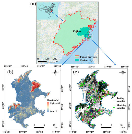
Figure 1.
The geographic location of the study area (a), digital elevation model (b), and spatial distribution of samples for model calibration and validation (c).
2.2. Soil Sample Collection
2.2.1. Sampling Design
Environmental factors including land patches, land cover, field accessibility, and soil texture were considered in designing the sampling scheme, which is based on the Technical Specification for Soil Environmental monitoring issued by the Ministry of Ecology and Environment in the People’s Republic of China [39]. For each sampling site (representing the typical land patch), quad-sampling was used for mixed soil samples of around 1 kg from 5 points distributed on the 4 corners and the center with the surface soil at 0–20 cm depth. A total of 70 mixed soil samples was collected by soil shovel (Figure 1c).
Among the 70 samples, 70% of the samples (n = 49) were randomly selected as the training set, and the remaining 30% of the samples (n = 21) were used as the test set to evaluate the prediction performance of the model. Figure 1c shows the spatial distribution of samples used for model calibration (training) and validation (testing).
2.2.2. Soil Sample Collection and Lab Analysis
Soil samples were collected from July 2013 and placed in labeled plastic bags, and the sampling process was all done on sunny days. The geographic coordinates of the center of each sampling site were recorded using a hand-held global positioning system (GPS) receiver. In the laboratory, the soil samples were air-dried for at least 48 h in a soil air-drying box; then, crushed stones, animal material, and plant residues were removed. The samples were then ground with an agate mortar and passed through a 100-mesh nylon sieve. Each soil sample’s total carbon (TC) was measured using an automated carbon and nitrogen elemental analyzer (Vario EL III CN). Inorganic carbon was measured by chemical method (neutralization titration method with 0.5 mol/L HCl, and 0.5 mol/L NaOH) [40]. Total organic carbon (TOC) was gained through the TC subtracting inorganic carbon. Finally, SOM was determined as 1.724 times TOC [41].
2.3. Environmental Variables
Optical satellite imagery and other ancillary data were collected to support the estimation of SOM (Figure 2).
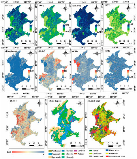
Figure 2.
Spatial distribution of environmental factors. Vegetation indices include the normalized deviation vegetation index (NDVI), differential vegetation index (DVI), ratio vegetation index (RVI), and modified soil adjusted vegetation index (MSAVI); topographical indices include the compound topographic index (CTI), stream power index (SPI), topographic roughness and topographic relief.
2.3.1. Remote Sensing Variables
A Level-1 Landsat 8 (OLI/TIRS) image (12 July 2013, Path 118/Row 42) was downloaded from USGS (https://earthexplorer.usgs.gov/, accessed on 13 September 2020). The time of this image acquisition was the same as that of soil sampling. The image preprocessing techniques, including geometric correction, topographic correction, radiometric calibration, and FLAASH atmospheric correction, were applied using ENVI 5.5. Vegetation indices (VIs) including normalized deviation vegetation index (NDVI), differential vegetation index (DVI), ratio vegetation index (RVI), and modified soil adjusted vegetation index (MSAVI) were calculated from the Landsat surface reflectance (Table 1). These VIs are highly correlated with canopy structure (e.g., leaf area index and biomass), which are the indicators of crop growing conditions. SOM can indirectly influence the changes of environmental variables affecting crop growth, thus resulting in the difference in VIs [22,42]. Therefore, considering the advantages and limitations (e.g., different vegetation indices have different sensitivity to vegetation coverage and soil background) of each vegetation index, we selected four of the most common VIs and explored their sensitivity to soil organic matter content (SOMC). Then, the sensitivity index was selected as a proxy of SOMC in the model to retrieve the final spatial distribution map.

Table 1.
Details of the vegetation and topographic indices.
In addition, the variability of SOM is affected by soil temperature [50]. In this study, land surface temperature (LST) derived from the Landsat 8 Thermal Infrared Sensor (TIRS) was considered in the SOM modeling. The single-window algorithm developed by Qin et al. [51] was used to calculate LST as follows:
where Ts is the true surface temperature in K; a (67.355351) and b (0.458606) are constants, [51]; C and D are intermediate variables; ε is the surface emissivity; τ is the atmospheric transmittance; T10 is the pixel brightness temperature detected by the sensor at the altitude of the satellite; Ta is the atmospheric mean temperature. According to the image acquisition time and location, the mid-latitude summer atmosphere estimation equation Ta = 16.0110 + 0.92621 × T0 was used [52]; ε was calculated by mixed pixel separation method [53]; τ was obtained by entering the transit time and center coordinates of the image on the National Aeronautics and Space Administration (NASA) website (https://atmcorr.gsfc.nasa.gov/, accessed on 21 September 2020).
2.3.2. Ancillary Data Collection
Ancillary datasets include soil type, land cover type, and DEM. Soil types (vector format) were obtained from Pingtan Nature Fund data by fieldwork. There were 9 soil types, but the main soil types were arenosols, ferralsols, and gleysols. Land cover information was extracted from Landsat 8 using the random forest method (Breiman 2001). The classified land cover types were forest, grassland, farmland, construction land, water body, and unused land. After classification, we randomly generated 420 test points, and carried out visual interpretation of land use types against Google Earth, taking them as true surface classes to evaluate the accuracy of classification (Table 2). The result showed that the overall accuracy of classification was 87.60% and the KAPPA coefficient was 0.84.
Table 2.
Error matrix of random forest classification results of land use map.
The ASTER Global Digital Elevation Model (DEM) data were downloaded from the Geospatial Data Cloud Platform, operated by the Chinese Academy of Sciences (http://www.gscloud.cn, accessed on 16 November 2020). The DEM has a spatial resolution of 30 m. Topography is an important factor in the spatial variation of soil properties [54]. Topography plays an important role in the redistribution of hydrothermal conditions and thus affects SOM, while climate and soil parent materials are relatively consistent on a regional scale [55]. Therefore, topographic factors are often considered model-independent variables in the prediction of the spatial distribution of many soil attributes. Here, topographic indices (roughness, relief, CTI, and SPI) were calculated using the spatial analyst tool in ArcGIS 10.6 as environmental factors (Table 1).
2.4. Analysis Methods
In general, the overall flowchart of the study was illustrated in Figure 3.
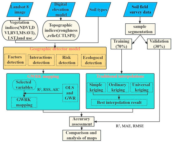
Figure 3.
The flowchart of the whole process in this research.
2.4.1. Sensitivity of Environmental Variables to SOM
The geographical detector model (GDM) is developed based on spatial variance analysis (SVA). It is a statistical method for assessing spatially stratified heterogeneity and revealing the driving factors behind spatial differentiation [56]. The GDM includes four geographical detectors named factor, interaction, risk, and ecological detectors. Factor detector, which is expressed by q statistic (Equation (4)), indicates that the X (environmental factors) can explain q × 100% spatial variation of Y (SOM). The range of q (0 to 1) increases as the strength of the stratified heterogeneity of Y caused by X increases.
where SSW and SST are the sums of the variances within the layer (class) and the total variance of the entire region, respectively; h = 1, L is the stratification of variable Y or factor X; Nh and N are the numbers of objects in each layer and the entire region, respectively.
The interaction detector detects interactions between factors to determine if two factors work together or independently to increase or decrease the explanatory power of the dependent variable. The risk detector is used to assess if the mean value of the attributes between two subregions is significantly different using a student t-test [56]. The ecological detector determines whether the influence of two factors on the spatial distribution of attribute Y is significantly different. The relevant calculations were made using the GeogDetector_2015 software (www.sssampling.org/geogdetector, accessed on 17 May 2020) [57]. These four detectors were used to identify the sensitive environment variables and thus predict SOM.
2.4.2. SOM Model Using Geostatistical Interpolation
Geostatistics, a branch of spatial statistics, has been widely used in soil science [58,59]. Geostatistics are statistical models that are based on regionalized variables and use a variable function to study random, structural, or spatially correlated and dependent natural phenomena [13]. The advantages of geostatistics are that they incorporate spatial and temporal coordinates of observations in data processing and can assess the uncertainty about the unsampled points [60].
The original SOM data must be converted if they do not conform to the normal distribution (the premise of applied geostatistics). Therefore, logarithmic transformation was implemented in the SOM dataset. The optimal model was selected from the ordinary kriging, simple kriging, and universal kriging methods through cross-validation to maximize the accuracy of the interpolation results. The best interpolation result was compared with the remote sensing inversion method. Kriging interpolation was done in ArcGIS 10.6 software.
2.4.3. SOM Modeling Using Remote Sensing
Geographically weighted regression kriging (GWRK) is a two-step hybrid approach integrating a geographically weighted regression (GWR) obtained from the estimation of the residuals with geostatistics by traditional kriging [61]. GWR is a spatial extension of Ordinary Least Squares (OLS). It considers the influence of spatial variability for regionally estimating regression parameters when establishing the regression equation. GWR and OLS were first analyzed to see whether SOM data of the study area has spatial heterogeneity. If GWR had better performance, heterogeneity would have existed. Then, GWRK was applied for mapping SOM.
GWRK has been proven to be more accurate and efficient for spatial prediction than regression kriging (RK) [61]. It includes two components, deterministic and stochastic. The deterministic component locally establishes the regression between a target variable and environmental factors to predict the trend of the target variable. The stochastic component is the residual term that can be interpolated by the kriging method. Prediction of the target variable was made by combining the residual term with the estimated results (Equation (6)).
where is the coordinate of the i-th sampling point, is the k-th regression parameter at the i-th sampling point, is the interpolation of residual term, is the influence factor, and is the target variable. The regression part was performed in GWR 4.0 software, and interpolation of residuals was implemented in ArcGIS 10.6 software.
2.4.4. Assessment of SOM Model Performance
The coefficient of determination (R2), residual sum of squares (RSS), and Akaike information criterion (AIC) were used to evaluate the performance of SOM models using OLS and GWR. R2, mean absolute error (MAE), and the root mean square error (RMSE) values were employed to assess the performance of SOM models using optimal kriging and GWRK. They were calculated as follows:
where and represent the predicted and measured values at sampling point i; represents the average value of measured value at sampling sites. L is the maximum likelihood under the model, and k is the number of variables in the model.
3. Results and Discussion
3.1. Statistical Characteristics of SOM
The measured SOM was found at a low level (1.03% on average, Table 3). The original data did not follow the normal distribution well. The positive skewness was concentrated on the left side of the mean, and the kurtosis was 4.69, indicating that the frequency distribution of the sampled data was steep. This was due to the high deviation of a few SOM samples from the mean, which was illustrated with a high coefficient of variation (0.91). After a logarithmic transformation, however, the data well followed the normal distribution.
Table 3.
Statistical characters of soil organic matter (SOM).
3.2. Spatial Characteristics of Environmental Variables
The environmental variables considered were vegetation indices, terrain indices, LST, soil types, and land use. These variables had clear spatial variability (Figure 2). The spatial pattern of vegetation indices was close to that of land cover type and LST. LAI value was different as the phenological stage of various vegetation types differs among land cover types. LST has a close relationship with LAI or vegetation growth. Therefore, LST showed a similar spatial pattern with the four vegetation indices.
In addition, the spatial pattern of topographic indices was also related to the vegetation indices and land use type. The reason was that the higher the terrain, the lower the interference of human activities, the less threatened the vegetation growth, and generally, the better it grows.
3.3. Sensitivity of Environmental Variables on SOM
The soil sampling points were used to extract the values of environmental variables from the corresponding locations. SOM was the dependent variable and environmental factors were the independent variables. The sample points with their environmental variables were put into the GDM for analysis.
3.3.1. Comparative Analysis of Explanatory Power
The q value of all environmental factors varied from 0.110 to 0.557 (Figure 4a). RVI had the highest q value (0.605), followed by NDVI (0.351), relief (0.317), MSAVI (0.314), and DVI (0.288). This t-test result implies the significant influence of RVI and DVI on SOM distribution. The remaining environmental factors, such as LST, terrain roughness, SPI, soil type, land use type, and CTI, had a weaker influence on SOM. The higher response of SOM to vegetation indices than other factors could be due to the direct relationship of higher vegetation indices with abundant plant residues that finally converted into SOM.
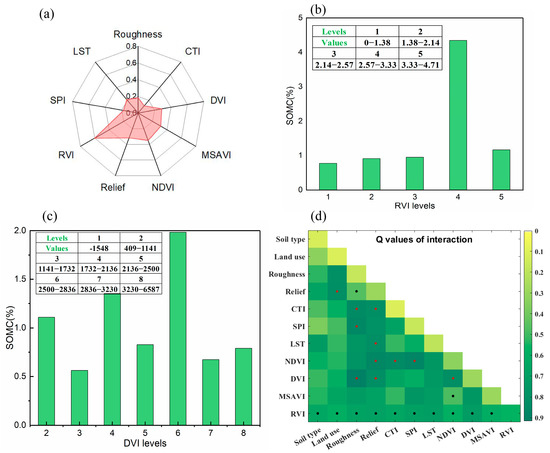
Figure 4.
Effects of different factors on the explanatory power of soil organic matter with the q value (a). SOM difference of RVI (b) and DVI (c) at different levels. q values of interaction between different influencing factors on soil organic matter (d). Black points indicate double-factor enhancement interaction. The red symbols indicate that the interaction q value is greater than 0.85.
3.3.2. The Influence of Environmental Factors on SOM
The influence of environmental factors on SOM was either antagonistic or synergistic, which can be identified by the q values of the interaction detection results (Figure 4d). Any two-factor interaction that can explain SOM more than a single factor was explored. The double-factor enhanced interactions were soil type∩RVI, land use∩RVI, roughness∩relief, roughness∩RVI, relief∩RVI, CTI∩RVI, SPI∩RVI, LST∩RVI, NDVI∩MSAVI, and NDVI∩RVI. We noticed that RVI frequently showed in double-factor enhanced interactions. The nonlinear enhanced interactions were roughness∩DVI (the highest q value of interaction, 0.916), roughness∩SPI, relief∩NDVI, and SPI∩NDVI, indicating that the interaction between vegetation factors (NDVI, DVI) and topographic factors (relief, roughness, SPI) could improve the ability of a single factor to explain SOM.
3.3.3. Risk and Ecological Analysis of SOM
The impact of environmental factors on SOM can be expressed by the results of the risk detector. The essence of risk detection was to compare the significance of the average SOM at different levels of environmental factors. The risk detector result showed that there was no significant difference (t-test) in SOM between different levels of land use, roughness, relief, NDVI, and MSAVI. Only one pair of levels in soil type, CTI, SPI, and LST factors showed a significant difference in SOM. However, DVI and RVI revealed obvious differences in SOM between different levels. The result was consistent with the analysis of factor detection that SOM had the highest response to both RVI and DVI.
Because of inadequate sampling points, only the top levels of RVI had the corresponding values. The risk detector showed paired levels with a very significant difference in SOM (for RVI, the following levels showed significant differences: 1–4, 2–4, 3–4 (Figure 4b); for DVI, the corresponding levers were 2–3, 2–8, 3–6, 6–7, 6–8 (Figure 4c). The SOM of the fourth level of DVI (1.35%) and the sixth level of the RVI (1.98%) showed a sharp increase. Both levels frequently occurred in the pairs of significant differences.
Ecological analysis using the F test at the level of 0.05 revealed that RVI was more sensitive to SOM than all the other factors. However, the explanatory power among other factors was not significant, which is consistent with the finding of the q values of comparative analysis. RVI was confirmed to have the best explanatory power for SOM in the study area.
3.4. SOM Estimation Model
3.4.1. Accuracy of SOM Estimation Using Interpolation
Semivariogram analysis was performed on the SOM to obtain the semivariogram parameters of the Gaussian, linear, exponential, and spherical models at isotropic and anisotropic (Table 4). The best Gaussian model was determined by the metrics including the decision coefficients (R2) and residuals (RSS). The estimated parameters of the semivariogram for each model showed that the nugget effect C0/(C0 + C) of Gaussian was 0.1% (between 0 and 25%), indicating that SOM in the study area has strong spatial autocorrelation. Kriging interpolation can be used to map the spatial distribution of SOM.
Table 4.
Semivariance model and parameters of soil organic matter.
Trend analysis was performed on SOM. The spatial interpolations using ordinary kriging, simple kriging, and universal kriging were cross-validated. There was no obvious SOM distribution trend. Ordinary kriging showed the best interpolation results, with the mean standardized error (MSE) closest to 0, small root mean square standardized error (RMSSE), mean error (ME) close to the root mean square error (RMSE), and average standard error (ASE) close to 1 (Figure 5).
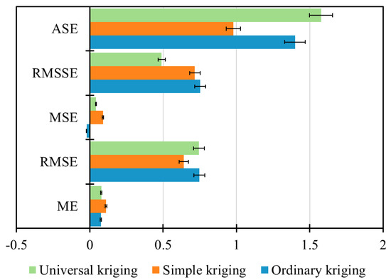
Figure 5.
Cross–validation results of different interpolation methods.
3.4.2. Accuracy of SOM Estimation Using Remote Sensing
OLS and GWR analysis were performed taking RVI (highest single factor explanatory power, higher risk power), DVI, and roughness (highest interaction explanatory power) as the independent variables and the SOM as the dependent variable. The GWR diagnostic indicators were significantly better than those of the OLS (Figure 6a). The residual sum of square decreased from 30.657 (OLS) to 24.621 (GWR), and the AIC values were 126.076 (OLS) and 120.417 (GWR); the determination coefficient was significantly improved from 0.265 (OLS) to 0.410 (GWR), indicating that the GWR local regression model accurately estimated SOM with a spatially non-stationary distribution. Compared with GWR, GWRK took into account the residual value and resulted in fine-resolution regional SOM mapping. The accuracy metrics of the GWRK model and optimal traditional kriging (OK) are shown in Figure 6b.
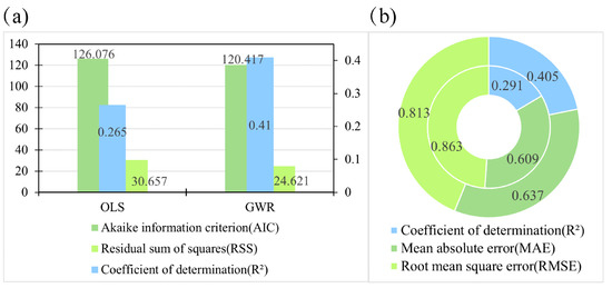
Figure 6.
Diagnostic criteria of ordinary least square regression (OLS) and geographically weighted regression (GWR) models (a). Accuracy assessment of ordinary kriging interpolation (OK) and geographically weighted regression kriging (GWRK) (b). The inner circle indicates OK, and the outer circle indicates GWRK.
Comparing the two models in SOM estimation performance, the R2 of GWRK was significantly greater than that of OK, whereas the MAE of OK was slightly better than that of GWRK. From the RMSE point of view, however, the GWRK value was smaller than that of OK. Overall, the result indicated that GWRK can obtain higher accuracy of SOM estimation than OK.
3.5. SOM Mapping and Comparison
Figure 7a,b show SOM maps derived from remote sensing data using OK and GWRK. To avoid errors in SOM estimation, we excluded impervious surfaces and water bodies. They were removed based on the global artificial impervious area result proposed by Gong et al. [62] and modified normalized difference water index.
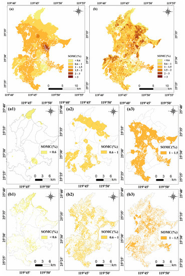
Figure 7.
Spatial distribution of soil organic matter content based on ordinary kriging (a) and geographically weighted regression kriging (b). Comparison maps of SOMC levels of ordinary kriging (a1–a3) and geographic weighted regression kriging (b1–b3).
The results showed that the spatial variability of the SOM map using OK is different from that using GWRK. Because of the inputs of environmental factors, especially the remotely sensed variables, a finer SOM map was obtained compared with the map using OK pure interpolation. To deeply analyze the difference between spatial recognition rate and spatial distribution structure, we generated patches and distribution maps of SOM levels.
The number of patches at all SOM levels was extracted to compare the spatial recognition rate (Table 5). Patches of GWRK increased significantly more than those of OK at all levels. Since OK is based on the interpolation of sample points, the results obtained had large spots, which can only reflect the overall spatial distribution of SOM on the island. Incorporating landscape geographic factors, GWRK can describe SOM of spatial variation in detail and hence give more precise predictions. The number of patches in the first level increased the least (73 times) and the number of patches in the last level increased the most (849 times). Overall, the spatial recognition rate (fineness) increased by more than 73 times (Table 5).
Table 5.
Number of patches at all soil organic matter levels in ordinary kriging (OK) and geographically weighted regression kriging (GWRK). Levels correspond to organic matter content <0.6% (1), 0.6–1% (2), 1–1.5% (3), 1.5–2% (4), 2–3% (5), and >3% (6).
The SOM with less than 1.5% accounted for 94.71% of the total area of the study. Therefore, the spatial distribution map of levels 1–3 was compared in detail to express the difference in SOM spatial structure (Figure 7a1–a3,b1–b3). The first three levels of OK and GWRK had similar spatial distribution trends except for forestland. Forestland was at a higher level (level 5) of GWRK, while at a lower level (level 2) of OK. This could be due to the addition of RVI and DVI to the GWRK model, which contributed to a high interpretation ability for SOM and more accurately identified the higher grade of SOM. Compared to OK, GWRK overestimated SOM in forestland to some extent, but this could be closer to the actual situation. Although the spatial distribution of OK and GWRK in other land use types showed similar patterns, the GWRK mapped a patchy, more detailed SOM distribution than the OK interpolation.
The result of SOM distribution, which depends on pure spatial interpolation, is unable to reasonably show the SOM spatial distribution. This is closely related to the sample size of SOM data collected from the field and the less spatial representation of the samples. However, with the incorporation of remote sensing and other environmental parameters, the spatial pattern of SOM mapping was improved greatly and its spatial distribution was more reasonable. Therefore, the GWRK method that combines environmental factors can be used for better prediction of the spatial distribution of SOM.
SOM spatial distribution based on GWRK had certain spatial similarities with vegetation indices and the roughness index. High SOM areas were primarily found in the gently sloped northeast and southwest regions under forest cover (Figure 7b). These regions had higher RVI and DVI, indicating more raw materials that can be converted into SOM. The SOM was less in extremely rough areas due to its exposure to high soil erosion. Although it was not considered in the model, the land cover has an impact on the distribution of SOM to a certain extent. For instance, SOM was found at a higher level in forests and farmland, while the opposite was true in unused land.
4. Conclusions and Recommendations
This study aims to estimate and map the spatial distribution of near-surface SOM on Pingtan Island with different underlying surfaces by using environmental variables (especially variables extracted from remote sensing data) with 70 sampling points. Environmental variables controlling SOM distribution on the island were explored using the GDM model, and selected factors were used in geographic weighted regression kriging (GWRK) to estimate SOM. The estimated SOM was compared with SOM using the traditional interpolation approach (ordinary kriging) to understand how we can improve the rationality and accuracy of SOM distribution. The research has reached the following conclusions:
(1) The average SOM in the study area was 1.03% with high spatial variability. GDM results showed that landscape structural factors (e.g., RVI, DVI∩roughness) played a major role in the spatial variability of SOM.
(2) RVI, DVI, and roughness were selected as the SOM spatial predictor variables. The GWRK model using these variables was more accurate (R2 = 0.405, MAE = 0.637, and RMSE = 0.813) to estimate the spatial distribution of SOM than conventional interpolation (e.g., OK) using soil samples alone (R2 = 0.291, MAE = 0.609, and RMSE = 0.863).
(3) The spatial pattern of the SOM map using the GWRK model was more reasonable than that of the OK model, and the spatial recognition rate of SOM patches at all levels using the GWRK method increased by more than 73 times compared with OK.
We conclude that the combination of limited SOM samples, remote sensing indices (e.g., vegetation indices), topographic data, GDM, and GWRK is a pragmatic approach for estimating regional-scale near-surface layer SOM. This study provides a practical method for SOM prediction in places with complex underlying surfaces on a regional scale and can be transferred to other regions by selecting appropriate variables considering the characteristics of the study area.
Despite the encouraging results obtained in this study, the proposed methodology has limitations. (1) Although 70 soil samples were sufficiently large for testing the robustness of the prediction model, a much larger number of soil samples should be collected across a wider range of geographical locations on the island in future studies. In addition, we only sampled the top soil layer in this study. Future sampling efforts will consider sampling from different depths of the soil profile to obtain the soil carbon pool and contribute to the carbon cycle and carbon-neutral research. (2) As Pingtan is a small regional-scale island, spatial correlation can affect the accuracy and precision of the SOM estimation. The estimation accuracy in this study was lower as compared to that of Lu et al. [30] and Li et al. [31]. This may be due to their study area being in a single land use type (e.g., hickory plantation region and cropland), but our study was conducted in areas with greater spatial heterogeneity, and more complex ground conditions in southern China. To improve the accuracy of SOM estimation, additional environmental factors, such as soil moisture, tree height, and underground LAI, will need to be considered in future studies.
Author Contributions
Conceptualization, J.F. and X.L.; methodology, J.F.; software, J.F.; validation, J.F., T.D., J.S. (Jiali Shang) and J.S. (Jinming Sha); formal analysis, J.F., T.D. and E.S.; investigation, X.L. and J.S. (Jinming Sha); resources, J.S. (Jinming Sha); data curation, J.S. (Jinming Sha); writing—original draft preparation, J.F. and Y.-C.S.; writing—review and editing, X.L., T.D., J.S. (Jiali Shang) and E.S.; visualization, J.F.; supervision, X.L. and J.S. (Jinming Sha); project administration, J.S. (Jinming Sha); funding acquisition, J.S. (Jinming Sha) and J.W. All authors have read and agreed to the published version of the manuscript.
Funding
This research was funded by Fujian-Taiwan Modelling Project (grant number A22E0870102B06).
Institutional Review Board Statement
Not applicable.
Informed Consent Statement
Not applicable.
Data Availability Statement
Soil organic matter content data is unavailable due to privacy reasons, so if you do need these data for further use, please contact the authors directly.
Conflicts of Interest
The authors declare no conflict of interest.
References
- Piccini, C.; Marchetti, A.; Francaviglia, R. Estimation of soil organic matter by geostatistical methods: Use of auxiliary information in agricultural and environmental assessment. Ecol. Ind. 2014, 36, 301–314. [Google Scholar] [CrossRef]
- Zhang, Z.; Yu, D.; Wang, X.; Pan, Y.; Zhang, G.; Shi, X. Influence of the Selection of Interpolation Method on Revealing Soil Organic Carbon Variability in the Red Soil Region, China. Sustainability 2018, 10, 2290. [Google Scholar] [CrossRef]
- Levi, N.; Karnieli, A.; Paz-Kagan, T. Using reflectance spectroscopy for detecting land-use effects on soil quality in drylands. Soil Tillage Res. 2020, 199, 104571. [Google Scholar] [CrossRef]
- Takata, Y.; Funakawa, S.; Akshalov, K.; Ishida, N.; Kosaki, T. Spatial prediction of soil organic matter in northern Kazakhstan based on topographic and vegetation information. Soil Sci. Plant Nutr. 2007, 53, 289–299. [Google Scholar] [CrossRef]
- Angst, G.; Messinger, J.; Greiner, M.; Häusler, W.; Hertel, D.; Kirfel, K.; Kögel-Knabner, I.; Leuschner, C.; Rethemeyer, J.; Mueller, C.W. Soil organic carbon stocks in topsoil and subsoil controlled by parent material, carbon input in the rhizosphere, and microbial-derived compounds. Soil Biol. Biochem. 2018, 122, 19–30. [Google Scholar] [CrossRef]
- Fu, M.; Tian, L.; Dong, G.; Du, R.; Zhou, P.; Wang, M. Modeling on Regional Atmosphere-Soil-Land Plant Carbon Cycle Dynamic System. Sustainability 2016, 8, 303. [Google Scholar] [CrossRef]
- Sainepo, B.M.; Gachene, C.K.; Karuma, A. Assessment of soil organic carbon fractions and carbon management index under different land use types in Olesharo Catchment, Narok County, Kenya. Carb Balance Manag. 2018, 13, 4. [Google Scholar] [CrossRef]
- Paul, O.O.; Sekhon, B.S.; Sharma, S. Spatial variability and simulation of soil organic carbon under different land use systems: Geostatistical approach. Agrofor. Syst. 2018, 93, 1389–1398. [Google Scholar] [CrossRef]
- Duan, L.; Li, Z.; Xie, H.; Yuan, H.; Li, Z.; Zhou, Q. Regional pattern of soil organic carbon density and its influence upon the plough layers of cropland. Land Degrad. Dev. 2020, 31, 2461–2474. [Google Scholar] [CrossRef]
- Long, J.; Liu, Y.; Xing, S.; Zhang, L.; Qu, M.; Qiu, L.; Huang, Q.; Zhou, B.; Shen, J. Optimal interpolation methods for farmland soil organic matter in various landforms of a complex topography. Ecol. Ind. 2020, 110, 105926. [Google Scholar] [CrossRef]
- Wu, Z.; Wang, B.; Huang, J.; An, Z.; Jiang, P.; Chen, Y.; Liu, Y. Estimating soil organic carbon density in plains using landscape metric-based regression Kriging model. Soil Tillage Res. 2019, 195, 104381. [Google Scholar] [CrossRef]
- Zhang, Y.; Ji, W.; Saurette, D.D.; Easher, T.H.; Li, H.; Shi, Z.; Adamchuk, V.I.; Biswas, A. Three-dimensional digital soil mapping of multiple soil properties at a field-scale using regression kriging. Geoderma 2020, 366, 114253. [Google Scholar] [CrossRef]
- Cambardella, C.A.; Moorman, T.B.; Novak, J.M.; Parkin, T.B.; Karlen, D.L.; Turco, R.F.; Konopka, A.E. Field-Scale Variability of Soil Properties in Central Iowa Soils. Soil Sci. Soc. Am. J. 1994, 58, 1501–1511. [Google Scholar] [CrossRef]
- Boubehziz, S.; Khanchoul, K.; Benslama, M.; Benslama, A.; Marchetti, A.; Francaviglia, R.; Piccini, C. Predictive mapping of soil organic carbon in Northeast Algeria. Catena 2020, 190, 104539. [Google Scholar] [CrossRef]
- Webster, R.; Oliver, M. Geostatistics for Environmental Scientists; John Wiley & Sons: Chichester, UK, 2001. [Google Scholar]
- Stoner, E.R.; Baumgardner, M.F. Characteristic Variations in Reflectance of Surface soils. Soil Sci. Soc. Am. J. 1981, 45, 1161–1165. [Google Scholar] [CrossRef]
- Stevens, A.; Udelhoven, T.; Denis, A.; Tychon, B.; Lioy, R.; Hoffmann, L.; van Wesemael, B. Measuring soil organic carbon in croplands at regional scale using airborne imaging spectroscopy. Geoderma 2010, 158, 32–45. [Google Scholar] [CrossRef]
- Dalmolin, R.S.D.; Gonçalves, C.N.; Klamt, E.; Dick, D.P. Relação entre os constituintes do solo e seu comportamento espectral. Ciênc. Rural 2005, 35, 481–489. [Google Scholar] [CrossRef]
- Krishnan, P.; Alexander, J.D.; Butler, B.J.; Hummel, J.W. Reflectance Technique for Predicting Soil Organic-Matter. Soil Sci. Soc. Am. J. 1980, 44, 1282–1285. [Google Scholar] [CrossRef]
- Alabbas, A.H.; Swain, P.H.; Baumgardner, M.F. Relating Organic-Matter and Clay Content to Multispectral Radiance of Soils. Soil Sci. 1972, 114, 477–485. [Google Scholar] [CrossRef]
- Yan, Y.; Yang, J.; Li, B.; Qin, C.; Ji, W.; Xu, Y.; Huang, Y. High-Resolution Mapping of Soil Organic Matter at the Field Scale Using UAV Hyperspectral Images with a Small Calibration Dataset. Remote Sens. 2023, 15, 1433. [Google Scholar] [CrossRef]
- Wang, S.; Zhuang, Q.; Jin, X.; Yang, Z.; Liu, H. Predicting Soil Organic Carbon and Soil Nitrogen Stocks in Topsoil of Forest Ecosystems in Northeastern China Using Remote Sensing Data. Remote Sens. 2020, 12, 1115. [Google Scholar] [CrossRef]
- Mallah Nowkandeh, S.; Noroozi, A.A.; Homaee, M. Estimating soil organic matter content from Hyperion reflectance images using PLSR, PCR, MinR and SWR models in semi-arid regions of Iran. Environ. Dev. 2018, 25, 23–32. [Google Scholar] [CrossRef]
- Chen, Y.; Li, Y.; Wang, X.; Wang, J.; Gong, X.; Niu, Y.; Liu, J. Estimating soil organic carbon density in Northern China’s agro-pastoral ecotone using vis-NIR spectroscopy. J. Soils Sediments 2020, 20, 3698–3711. [Google Scholar] [CrossRef]
- Cheng, B.; Jiang, Q.; Wang, K. Application and Progress in Estimating Soil Organic Matter Content Based on Remote Sensing. J. Shandong Agric. Univ. Nat. Sci. 2011, 42, 317–321. [Google Scholar]
- Wang, D.; Li, X.; Zou, D.; Wu, T.; Xu, H.; Hu, G.; Li, R.; Ding, Y.; Zhao, L.; Li, W.; et al. Modeling soil organic carbon spatial distribution for a complex terrain based on geographically weighted regression in the eastern Qinghai-Tibetan Plateau. Catena 2020, 187, 104399. [Google Scholar] [CrossRef]
- Mirchooli, F.; Kiani-Harchegani, M.; Khaledi Darvishan, A.; Falahatkar, S.; Sadeghi, S.H. Spatial distribution dependency of soil organic carbon content to important environmental variables. Ecol. Ind. 2020, 116, 106473. [Google Scholar] [CrossRef]
- Paul, S.S.; Dowell, L.; Coops, N.C.; Johnson, M.S.; Krzic, M.; Geesing, D.; Smukler, S.M. Tracking changes in soil organic carbon across the heterogeneous agricultural landscape of the Lower Fraser Valley of British Columbia. Sci. Total Environ. 2020, 732, 138994. [Google Scholar] [CrossRef]
- Zhou, Y.; Hartemink, A.E.; Shi, Z.; Liang, Z.Z.; Lu, Y.L. Land use and climate change effects on soil organic carbon in North and Northeast China. Sci. Total Environ. 2019, 647, 1230–1238. [Google Scholar] [CrossRef]
- Lu, W.; Lu, D.S.; Wang, G.X.; Wu, J.S.; Huang, J.Q.; Li, G.Y. Examining soil organic carbon distribution and dynamic change in a hickory plantation region with Landsat and ancillary data. Catena 2018, 165, 576–589. [Google Scholar] [CrossRef]
- Li, X.Y.; Shang, B.B.; Wang, D.Y.; Wang, Z.M.; Wen, X.; Kang, Y.D. Mapping soil organic carbon and total nitrogen in croplands of the Corn Belt of Northeast China based on geographically weighted regression kriging model. Comput. Geosci. 2020, 135, 104392. [Google Scholar] [CrossRef]
- Tan, X.; Guo, P.T.; Wu, W.; Li, M.F.; Liu, H.B. Prediction of soil properties by using geographically weighted regression at a regional scale. Soil Res. 2017, 55, 318–331. [Google Scholar] [CrossRef]
- Costa, E.M.; Tassinari, W.D.; Pinheiro, H.S.K.; Beutler, S.J.; dos Anjos, L.H.C. Mapping Soil Organic Carbon and Organic Matter Fractions by Geographically Weighted Regression. J. Environ. Qual. 2018, 47, 718–725. [Google Scholar] [CrossRef]
- Fotheringham, A.S.; Brunsdon, C.; Charlton, M.E. Geographically Weighted Regression: The Analysis of Spatially Varying Relationships; Wiley: Chichester, UK, 2002. [Google Scholar]
- Zhang, Z.P.; Ding, J.L.; Wang, J.Z.; Ge, X.Y. Prediction of soil organic matter in northwestern China using fractional-order derivative spectroscopy and modified normalized difference indices. Catena 2020, 185, 104257. [Google Scholar] [CrossRef]
- Camera, C.; Zomeni, Z.; Noller, J.S.; Zissimos, A.M.; Christoforou, I.C.; Bruggeman, A. A high resolution map of soil types and physical properties for Cyprus: A digital soil mapping optimization. Geoderma 2017, 285, 35–49. [Google Scholar] [CrossRef]
- Pudelko, A.; Chodak, M. Estimation of total nitrogen and organic carbon contents in mine soils with NIR reflectance spectroscopy and various chemometric methods. Geoderma 2020, 368, 114306. [Google Scholar] [CrossRef]
- Shifaw, E.; Sha, J.M.; Li, X.M.; Bao, Z.C.; Zhou, Z.L. An insight into land-cover changes and their impacts on ecosystem services before and after the implementation of a comprehensive experimental zone plan in Pingtan island, China. Land Use Policy 2019, 82, 631–642. [Google Scholar] [CrossRef]
- HJ/T 106-2004; Technical Specifications for Soil Environmental Monitoring. Ministry of Ecology and Environmentthe People’s Republic of China: Beijing, China, 2004.
- Zheng, G.; Li, L.; Chen, J.; Hu, F. Teaching research on determination of soil organic matter content in analytical chemistry experiment. Exp. Technol. Manag. 2018, 35, 203–207. [Google Scholar]
- Bao, S. Soil in Agricultural Chemistry, 3rd ed.; China Agriculture Press: Beijing, China, 2000. [Google Scholar]
- Silatsa, F.B.T.; Yemefack, M.; Tabi, F.O.; Heuvelink, G.B.M.; Leenaars, J.G.B. Assessing countrywide soil organic carbon stock using hybrid machine learning modelling and legacy soil data in Cameroon. Geoderma 2020, 367, 114260. [Google Scholar] [CrossRef]
- Rouse, J.; Haas, R.H.; Schell, J.A.; Deering, D.W. Monitoring Vegetation Systems in the Great Plains with ERTS; NASA Speceial Publication: New York, NY, USA, 1973; Volume 351, p. 309. [Google Scholar]
- Richardson, A.J.; Wiegand, C. Distinguishing vegetation from soil background information. Photogramm. Eng. Remote Sens. 1977, 43, 1541–1552. [Google Scholar]
- Jordan, C.F. Derivation of leaf-area index from quality of light on the forest floor. Ecology 1969, 50, 663–666. [Google Scholar] [CrossRef]
- Qi, J.; Chehbouni, A.; Huete, A.R.; Kerr, Y.H.; Sorooshian, S. A Modified Soil Adjusted Vegetation Index. Remote Sens. Environ. 1994, 48, 119–126. [Google Scholar] [CrossRef]
- Tang, Q.; Li, W.; Chen, W.; Wang, N. Roughness analysis of Luzhou City under different DEM resolutions. Rural Econ. Technol. 2017, 28, 17–19. [Google Scholar]
- Su, X.; Wie, W.H.; Guo, W.Q.; Wang, S.Y.; Wang, G.Y.; Wu, W.; Ye, W. Analyzing the impact of relief amplitude to loess landslides based on SRTM DEM in Tianshui Prefectur. Glac. Frozen Soil 2017, 39, 616–622. [Google Scholar]
- Moore, I.D. Soil attribute prediction using terrain analysis. Soil Sci. Soc. Am. J. 1993, 57, 443–452. [Google Scholar] [CrossRef]
- Yang, H.; He, N.; Li, S.; Yu, G.; Gao, Y.; Wang, R. Impact of Land Cover on Temperature and Moisture Sensitivity of Soil Organic Matter Mineralization in Subtropical Southeastern China. J. Res. Ecol. 2016, 7, 85–91. [Google Scholar]
- Qin, Z.H.; Zhang, M.; Arnon, K.; Pedro, B. Mono-window algorithm for retrieving land surface temperature from Landsat TM6 data. Acta Geogr. Sin. 2001, 56, 446–456. [Google Scholar]
- Qin, Z.-H.; Li, W.J.; Zhang, M.-H.; Karnieli, A.; Berliner, P. Estimating of the essential atomospheric parameters of mono-window algorithm for land surface temperature retrieval from Landsat TM6. Remote Sens. Land Res. 2003, 15, 37–43. [Google Scholar]
- Song, C.; Qin, Z.; Wang, F. An effective method for LST decomposition based on the linear spectral mixing model. J. Infrared Millim. Waves 2015, 34, 497–504. [Google Scholar]
- Song, X.; Li, L.-D.; Kou, C.-L.; Chen, J. Soil nutrient distribution and its relations with topography in Huangshui River drainage basin. Chin. J. Appl. Ecol. 2011, 22, 3163–3168. [Google Scholar]
- Yang, Q.; Wu, W.; Liu, H. Prediction of spatial distribution of soil available iron in typical hilly farmland using terrain attributes and random forest model. Chin. J. Eco-Agric. 2018, 26, 422–431. [Google Scholar]
- Wang, J.F.; Li, X.H.; Christakos, G.; Liao, Y.L.; Zhang, T.; Gu, X.; Zheng, X.Y. Geographical Detectors-Based Health Risk Assessment and its Application in the Neural Tube Defects Study of the Heshun Region, China. Int. J. Geogr. Inf. Sci. 2010, 24, 107–127. [Google Scholar] [CrossRef]
- Wang, J.-F.; Hu, Y. Environmental health risk detection with GeogDetector. Environ. Model. Softw. 2012, 33, 114–115. [Google Scholar] [CrossRef]
- Rodríguez Martín, J.A.; Álvaro-Fuentes, J.; Gabriel, J.L.; Gutiérrez, C.; Nanos, N.; Escuer, M.; Ramos-Miras, J.J.; Gil, C.; Martín-Lammerding, D.; Boluda, R. Soil organic carbon stock on the Majorca Island: Temporal change in agricultural soil over the last 10 years. Catena 2019, 181, 104087. [Google Scholar] [CrossRef]
- Chen, L.; Ren, C.; Li, L.; Wang, Y.; Zhang, B.; Wang, Z.; Li, L. A Comparative Assessment of Geostatistical, Machine Learning, and Hybrid Approaches for Mapping Topsoil Organic Carbon Content. ISPRS Int. J. Geo-Inf. 2019, 8, 174. [Google Scholar] [CrossRef]
- Lark, R.M. Towards soil geostatistics. Spat. Stat. 2012, 1, 92–99. [Google Scholar] [CrossRef]
- Mitran, T.; Mishra, U.; Lal, R.; Rabisankar, T.; Sreenivas, K. Spatial distribution of soil carbon stocks in a semi-arid region of India. Geod. Reg. 2018, 15, e00192. [Google Scholar] [CrossRef]
- Gong, P.; Li, X.; Wang, J.; Bai, Y.; Chen, B.; Hu, T.; Liu, X.; Xu, B.; Yang, J.; Zhang, W.; et al. Annual maps of global artificial impervious area (GAIA) between 1985 and 2018. Remote Sens. Environ. 2020, 236, 111510. [Google Scholar] [CrossRef]
Disclaimer/Publisher’s Note: The statements, opinions and data contained in all publications are solely those of the individual author(s) and contributor(s) and not of MDPI and/or the editor(s). MDPI and/or the editor(s) disclaim responsibility for any injury to people or property resulting from any ideas, methods, instructions or products referred to in the content. |
© 2023 by the authors. Licensee MDPI, Basel, Switzerland. This article is an open access article distributed under the terms and conditions of the Creative Commons Attribution (CC BY) license (https://creativecommons.org/licenses/by/4.0/).