An Improved Approach of Integrated Carrying Capacity Prediction Based on TOPSIS-SPA

Abstract

Regional coordinated development is an important policy to promote socio-economic development, especially in the Yangtze River Delta, Greater Bay Area and others, which is one of the guidelines of the 14th Five-Year Plan for economic development. The relative stability of the carrying capacity (CC) is the precondition for long-term rapid development, whereas the comprehensive capacity of natural resources, ecological environment, social economy, population and others, defined as integrated carrying capacity (ICC). Due to the complexity of the CC quantitative assessment, constructing an accurate ICC predication model is the core challenge of dynamic adjustments of socio-economic development planning. In this study, four critical issues, which focused on indicator value estimation, optimal ICC value screening, ICC tendency prediction and study area application in order to formulate a novel prediction framework, are investigated as follows: (1) The proposal formulated an estimation model of indicator value in the future based on the grey model. The grade ratio and the relative residuals of all third-class indicators are less than 0.1, which is highly accurate for indicator value estimation. (2) The optimal ICC value screening model was proposed based on the multi-objective decision-making theory. The optimal ICC values of Suzhou, Ningbo and Zhoushan were 0.7002, 0.6797 and 0.5982, which were also the maximum values from 1996 to 2019. However, the values of Nantong, Jiaxing and Shaoxing were recorded in 2018, 2001 and 1999, which were not the maximum ICC values, and the difference ratio was more than 10%. The optimal ICC value of these three cities were improved. (3) The ICC prediction model was constructed based on the theory of set pair analysis and Euclidean distance. The ICC prediction result of eight cities maintained a relative fluctuation during 2020–2030. Compared with the polynomial fitting curve predication, there were some differences in Nantong, Shaoxing and Zhoushan over the next 5 years. This study provided an improved approach of ICC prediction model, focusing on indicator weight, indicator data estimation and optimal ICC value screening. The model and conclusion aim to validate the rationality of economic planning target for government policymakers and stakeholders.

1. Introductions

The process of urbanization and industrialization led to the over-exploitation resources, environmental disruption, fragile ecosystem and so forth. In rapidly developing cities, the natural resource has approached the maximum threshold, which will make a bottleneck on long-term sustainable development. By 2030, the resource demands of water and land for urbanization construction should increase by 2.45 times in China, and the ecosystem over-loaded pressure by 1.42 times [1]. In the formulation process of development planning outlines, the policymakers and stakeholders of the Chinese government have to face increased restrictions of resource shortages, supply side relationships and environmental pollution.

The concept of carrying capacity (CC) originated from the limit of the growth of a population [2]. Over the past century, especially in land, water, agriculture, transportation, environment, population, ecology, marine and other resources [3,4,5,6,7,8,9,10,11,12], the theoretical model and the application field of CC have been continuously extended. The Pressure-State-Response (PSR) model is the first framework to describe the dynamic interrelation of each ecological subsystem, and has been refined to DPSIR incorporated the ecosystem driving force and human influence [13]. In order to support long-term sustainable development, the government need more effective control policies to alleviate the pressure of human activities. Thus, we constructed the Driving-Force-Pressure-State-Response-Control (DPSRC) model to evaluate the natural resource CC of land, shoal and marine in coastal area [14]. As the problems of natural resource depletion and environmental degradation were increasing prominently, some scholars began to study the comprehensive status of serval subsystem, such as city and metropolitan area [15,16], land resource [17], water resource [18], and environment [19,20]. These studies mainly focus on the single subsystem carrying capacity status, which cannot represent all influence factors of the whole ecosystem and cannot been as a reference for the future development planning formulation. We defined the integrated carrying capacity (ICC) as a comprehensive capacity of resources, environment, ecology, economy and social in a given period, which could support long-term sustainable development [21].

The sustainable development strategy is an important criterion for the socio-economic development of China. In the governmental report, the ICC assessment result is a credible reference so that the economic development goals and land resource utilization are scientifically reasonable (http://www.mnr.gov.cn/dt/ywbb/201905/t20190523_2413001.html, accessed on 25 February 2022; http://www.xinhuanet.com/politics/leaders/2019-08/31/c_1124945382.htm; accessed on 25 February 2022). At present, the ICC research includes two parts of status evaluation and tendency predication, and the predication method mainly focuses on mean squared error decision [17], grey system (GM) and autoregressive integrated moving average [22], set pair analysis (SPA) [23,24], system dynamic model [25,26,27], gray correlation analysis and multiple linear regression [9] and technique for order preference by similarity to an ideal solution (TOPSIS) [28]. However, there are some imperfections in the existing methods. First, the weighted of each indicator should integrate qualitative method and quantitative method, which can really refer the rank of indicator importance. Second, from the existed studies, the ICC predication mainly depends on the linear and nonlinear relationship of ICC status evaluation results, which cannot reveal the dynamic changing process of resource, economy, environment, society and human activity; on the other hand, the ICC predication is based on each subsystem, which reflects a responsible systemic process. We developed a dynamic ICC prediction model based on the SPA model [23], but the resulting accuracy relies on all indicators’ pre-estimated data and optimal ICC reference value. Third, only a small amount of indicator data can be found in government development planning in the future, but most of them should be pre-estimated.

In view of the existing shortcomings, we proposed an improved approach to the ICC prediction model based on the pre-estimated indicator data and optimal ICC reference value screening. Combining subjective analysis and objective calculation, the indicator weight calculation method was improved, which reduced the difference in indicator function positioning. The indicator data in the future were estimated by using the GM model, based on the grade ratio of the indicator data and least-squares principle. Following the optimal ICC reference value based on the closeness coefficient between the evaluation result and the optimal value, the ICC was predicted by using the TOPSIS-SPA model. Taking eight coastal cities in the Yangtze River Delta as the research object, the ICC changing tendency during 2020–2030 was predicated. The methodology flowchart is shown in Figure 1.

Figure 1. Flow chart of the proposed methodology in this study.

This improved approach is an effective method to evaluate and predicate ICC, which is based on the historic ICC status and indicator’s data trend. The predication result of ICC is an important reference for socio-economic development planning and maintaining long-term sustainable development targets. Based on the ICC predication result, the government policymakers and stakeholders can adjust economic development target, financial investment, environmental protection, to keep the balance between social development and ecological health for a long time.

2. Indicator and Data

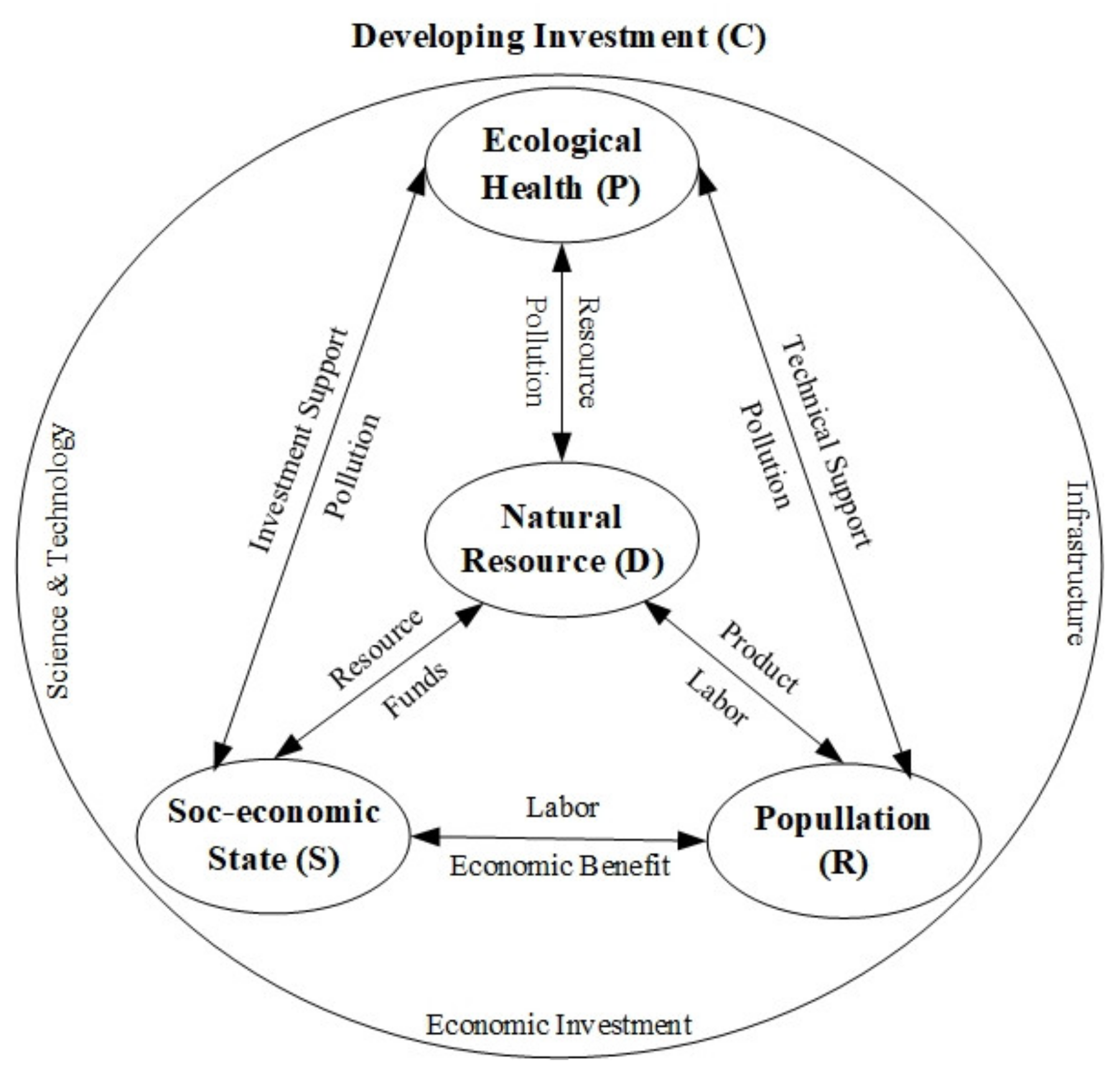
In our previous studies, we have proposed an indicator system of ICC based on DPSRC framework, and been improved based on the data availability and application validation [14,21,23]. After a summary analysis, we constructed the relationship between the first-class indicator and the DPSRC framework, especially in the dynamic changing process with socio-economic development (Figure 2). This framework is divided into five subsystems of natural resources (D), ecological environment (P), socio-economic development (S), population (R) and developing investment (C). The natural resource subsystem supply farmland, construction land, water, fishery, vegetation coverage to support socio-economic development and human life demand. Based on the labor workforce from the population subsystem, the natural resources are converted into socio-economic benefit. However, the over-utilization of natural resources generates some ecological environment pollution of industrial wastewater, SO₂ and solid waste discharge, so that the ICC tends to decrease. Through the new technical support and the economic investment, the pollution problem is resolved, and the ICC is gradual recovered. In the whole system, the total amount of natural resource, the scale of economic development, the health of ecological environment and human activities are controlled by the government developing investment. The relatively balance between economic development scale and ICC status is dynamically regulated based on the infrastructure condition, science technology and financial investment.

Figure 2. Basic framework of DPSRC.

Based on this framework, the index system was constructed by using some representative indicator, and shown in Table 1. The indicator screening principle included comparability, data availability and quantification. In the subsystem of natural resources, we chose farmland area, construction area, water, vegetation coverage ratio and fishery resource, which were same resource to support social development in eight cities. The industrial wastewater discharge, industrial SO₂ emissions and solid waste discharge were the most common ecological environment problems. The gross domestic product (GDP) is the most common indicator used to reflect the socio-economic scale. We chose GDP, growth rate of GDP, total output of agricultural, total output of fishery and Engel coefficient as evaluation indicators for the socio-economic subsystem. In population subsystem, we chose the total population and the labor density as the primary indicator. In developing investment subsystems, four indicators of education, science and technological, actual utilized foreign investment, public budget expenditure were chosen as financial policies to adjust the balance between economic development and ecological health, and three further indicators of volume of port cargo handled, medical level and density of highway formed the basis of socio-economic development. Based on the suitability validation of each third-class indicator in our previous studies [14,21,23], the screened index system was proposed, including 27 third-class indicators in five dimensions.

Table 1. The index system of ICC in this study.

First-Class Indicator	Second-Class Indicator	Third-Class Indicator
natural resource (D)	land resource	farmland area per capita
		construction area per capita
	marine resource	fishery resource
	water resource	land water area
	vegetation resource	vegetation coverage ratio
ecological environment (P)	environmental pollution	industrial wastewater discharge
		industrial SO2 emission
		solid waste discharge
	energy consumption	energy consumption per unit GDP
socio-economic (S)	economic level	GDP
		growth rate of GDP
		total output of agricultural
		total output of fishery
	people’s living condition	GDP per capita
		Engel coefficient
population (R)	population	total population
		population density
	labor force density	proportion of labor employment
		proportion of S and T personnel
		proportion of agriculture, forestry, husbandry and fishery personnel
developing investment (C)	science and technology	proportion of education investment
		proportion of S and T investment
	financial investment	actual utilized foreign investment
		public budget expenditure
	infrastructure condition	volume of port cargo handled
		medical development level
		density of highway

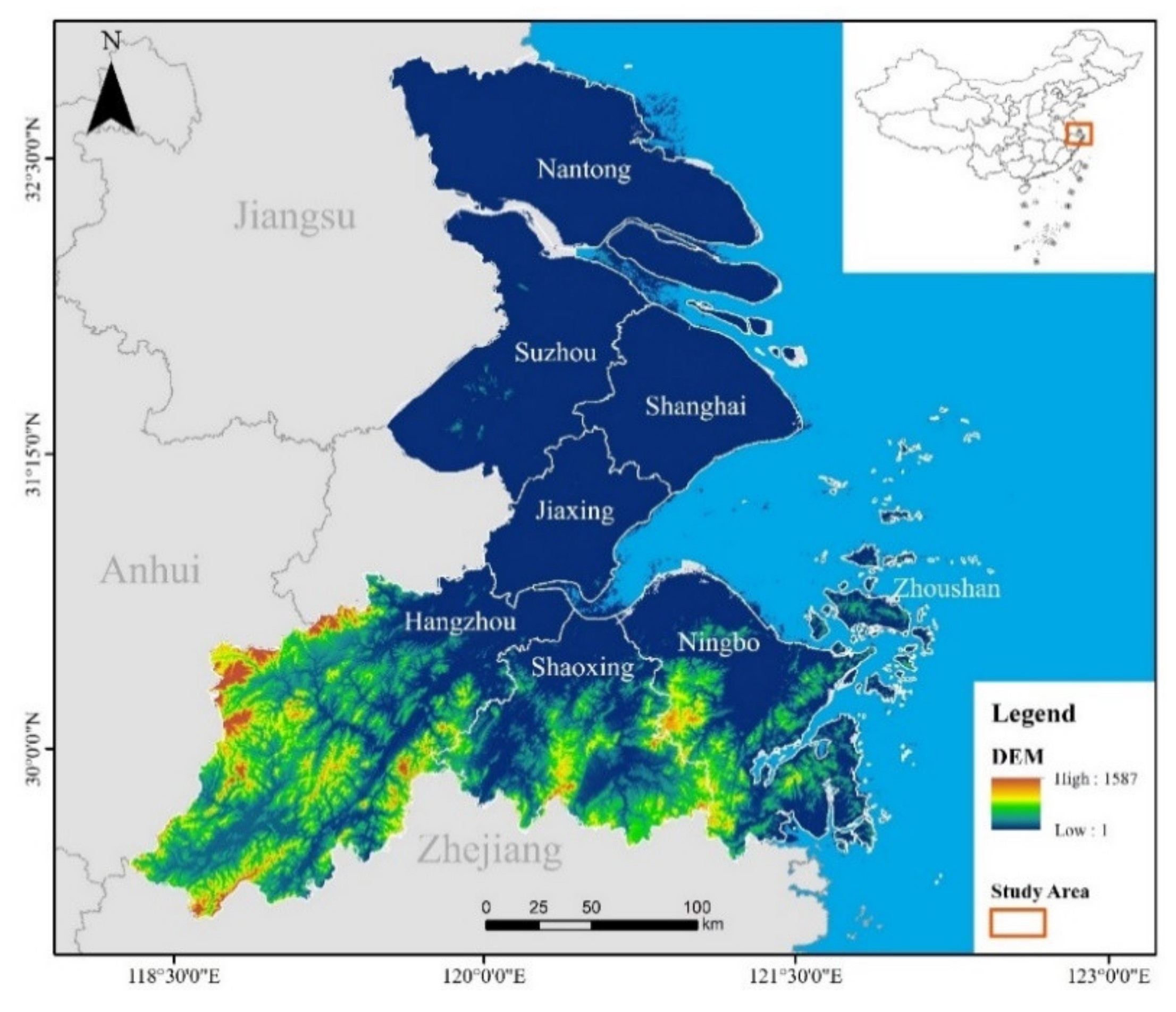
The Yangtze River Delta is located in eastern China (Figure 3), composed of four provinces. In 2018, the integrated development of the Yangtze River Delta had been upgraded to a national strategy and proposed at the first China International Import Expo. On the background of the most high-speed economic development, the difference of each city’s ICC was gradually widened, due to the exchange of natural resources. In this study, we took eight coastal cities as research objects, namely, Nantong, Suzhou, Shanghai, Jiaxing, Hangzhou, Shaoxing, Ningbo and Zhoushan. Most of the indicators’ data during 1996–2019 was obtained from the Statistical Yearbook of eight cities [29,30,31,32,33,34,35,36], Government Statistical Bulletin, Marine Bulletin [37] and historical data. Moreover, these data were also obtained from official government reports and statistics bureau (https://data.stats.gov.cn/; accessed on 25 February 2022). Meanwhile, the indicator’s value of vegetation coverage and land water were directly extracted from remote sensing imagery (http://www.gscloud.cn; accessed on 25 February 2022). Based on the correlation analysis and linear tendency, the data error and the extreme value correction were carried out.

Figure 3. Thematic map of the study area.

3. Methodology

Based on the proposed methodology flowchart (Figure 1), there are three critical algorithm models in ICC predication, including the indicator’s weight, indicator’s data pre-estimation and ICC predication. Moreover, the data preprocessing and ICC calculation are based on our previous studies.

3.1. Indicator Weight

The indicator weight represents the importance ranking of each evaluation element in the research object. We proposed a weight calculation method based on the entropy method (EM). However, the weight depended very much on the difference in each indicator’s data; thus, the result showed some shortcomings. The farther the indicator data from the optimal value of all objects, the smaller their weight result. Due to the developing speed difference of eight cities, even if the indicator data are greater, the weight result cannot reflect the actual importance rank of evaluation indicator. Meanwhile, the subjective calculation method of weight is based on the researcher’s experience to judge the sequence of each indicator, which describes a relatively justifiable sequence, the same as public conventional judgement.

Combining subjective and objective methods, the improved weight calculation formulation was defined as follows:

$$w=\frac{w^{AHP}\times w^{EM}}{{\displaystyle \sum _{i=1}^m{w}^{AHP}\times w^{EM}}}$$

(1)

where $w$ was the indicator weight calculation result, $w^{AHP}$ was the indicator weight by using Analytic Hierarchy Process (AHP) model and $w^{EM}$ was the indicator weight by using the EM model.

3.2. Indicator Data Pre-Estimation

The Grey System theory was developed by Deng [38]. Based on the accumulation sequence of original data, the grey development coefficient and the grey control parameter were calculated by using a differential equation, to construct the exponential equation and predict data changing tendency. This model has been applied in prediction of movement speed, traffic flow, water consumption and COVID-19 condition [24,39,40,41,42,43,44]. In the time series analysis, the basic grey model was the first order and one variable equation, which was referred to as $GM\left(1,1\right)$.

The ICC reflected a comprehensive capacity of natural ecosystem to support socio-economic development. From 1996 to 2019, each set of indicator data was a relatively independent nonlinear sequence by time series. The modeling process of indicator data predication in the next 10 years was as follows:

(1)

Total number of prediction data

Suppose $X=(x(1),x(2),\cdots ,x(t))$ as a sequence of one indicator’s data. The grade ratio was defined as follows:

$$\lambda (j)=\frac{x(j-1)}{x(j)}, (j=2,3,\cdots ,t)$$

(2)

where $\lambda (j)$ was the grade ratio of indicator data sequence.

Thus, the grade ratio set based on the third-class indicator was defined as follows:

$$\lambda =\left[\begin{array}{cccc}{\lambda }_1(2)& {\lambda }_1(3)& \cdots & {\lambda }_1(t)\\ {\lambda }_2(2)& {\lambda }_2(3)& \cdots & {\lambda }_2(t)\\ ⋮& ⋮& \cdots & ⋮\\ {\lambda }_m(2)& {\lambda }_m(3)& \cdots & {\lambda }_m(t)\end{array}\right]$$

(3)

where $m$ was the total number of indicators. Only each $\lambda (j)$ belonged to $[e^{\frac{-2}{t+1}},e^{\frac{2}{t+1}}]$, the indicator data could be satisfied with the GM model requirement.

Taking 2019 as the base year, the ratio of eight cities were calculated. Adding indicator data one by one year, until to 1996, all ratios were calculated and checked. While these did not match the requirement, the total amount of prediction data was obtained.

(2)

Indicator data pre-estimation

Suppose $X^0=(x^0(1),x^0(2),\cdots ,x^0(n))$ as a sequence set of one indicator evaluation data, and $X^1=(x^1(1),x^1(2),\cdots ,x^1(n))$ was the accumulation result of data sequence. Then, the formulation of $X^1$ was defined as follows:

$$x^1\left(k\right)={\displaystyle \sum _{i=1}^k{x}^0\left(i\right)}, \left(k=1,2,\cdots ,n\right)$$

(4)

where $n$ is the total number of evaluation data.

Then, (Equation (4)) defines the difference equation of $GM\left(1,1\right)$.

$$x^0\left(k\right)+a{z}^1\left(k\right)=b, \left(k=1,2,\cdots n\right)$$

(5)

where $a$ was the grey development coefficient, $b$ was the grey control parameter and $z^1\left(k\right)$ was the element neighbor value of generation sequence $x^1\left(k\right)$. Using the mean weight, the formulation of $z^1\left(k\right)$ was defined as follows:

$$z^1\left(k\right)=\frac{x^1\left(k-1\right)+x^1\left(k\right)}{2}, (k=2,3,\cdots ,n)$$

(6)

where $z^1\left(1\right)=x^1\left(1\right)$.

Based on the least square estimation, $a$ and $b$ were defined as follows:

$$\mu =\left[\begin{array}{c}a\\ b\end{array}\right]={\left(B^{T}B\right)}^{-1}{B}^{T}Y$$

(7)

$$B=\left[\begin{array}{c}\begin{array}{cc}-z^1\left(2\right)& 1\end{array}\\ \begin{array}{cc}-z^1\left(3\right)& 1\end{array}\\ \begin{array}{cc}⋮& ⋮\end{array}\\ \begin{array}{cc}-z^1\left(n\right)& 1\end{array}\end{array}\right]$$

(8)

$$Y=\left[\begin{array}{c}{x}^0\left(2\right)\\ x^0\left(3\right)\\ ⋮\\ x^0\left(n\right)\end{array}\right]$$

(9)

Suppose $\stackrel{\wedge }{x^0}(k)$ as the time response sequence and $\stackrel{\wedge }{x^1}(k)$ referred to the accumulated response sequence. At time $k$, which was current year or future, the formulation was defined as follows:

$$\stackrel{\wedge }{x^1}(k)=\left(\stackrel{\wedge }{x^0}(1)-\frac{b}{a}\right)\times e^{-a\times \left(k-1\right)}+\frac{b}{a}, \left(k=2,3,\cdots ,n\right)$$

(10)

According (Equation (6)), the indicator estimation restored data was calculated as follows:

$$\stackrel{\wedge }{x^0}(k)=\stackrel{\wedge }{x^1}(k)-\stackrel{\wedge }{x^1}(k-1), \left(k=2,3,\cdots ,n\right)$$

(11)

where $\stackrel{\wedge }{x^0}(1)=\stackrel{\wedge }{x^1}(1)=x\left(1\right)$. In Equation (10), if $k$ is less than total number of prediction data, the result $\stackrel{\wedge }{x^0}(k)$ was used to assess model accuracy. On contrary, the result was used to estimate indicator data of the next few years.

(3)

Accuracy assessment

The relative residual $\epsilon \left(k\right)$ and deviation $\rho \left(k\right)$ of grade ratio were to assess the accuracy of estimation model. The formulations were defined as follows:

$$\epsilon \left(k\right)=\frac{x^0\left(k\right)-\stackrel{\wedge }{x^0}(k)}{x^0\left(k\right)}, \left(k=1,2,\cdots ,n\right)$$

(12)

where $x^0\left(k\right)$ was the indicator original data and $\stackrel{\wedge }{x^0}(k)$ was the indicator estimation result based on $GM\left(1,1\right)$.

$$\rho \left(k\right)=1-\frac{1-0.5\times a}{1+0.5\times a}\times \lambda \left(k\right), \left(k=1,2,\cdots ,n\right)$$

(13)

where $a$ was from (Equation (7)) and $\lambda \left(k\right)$ from (Equation (2)).

In this study, the accuracy of indication estimation result was a high level only if all absolute values of $\epsilon \left(k\right)$ or $\rho \left(k\right)$ were less than 0.1, and the accuracy was an ordinary level when all coefficients are less than 0.2. Moreover, the accuracy did not satisfy with the indicator data estimation requirement of GM model, so that it could not be used to estimate the ICC in the future year.

3.3. ICC Prediction Based on TOPSIS-SPA

Based on the evaluation indicator system, the ICC was composed of each third-class indicator’s CC. The component of the ecosystem was inter-connected and affect each other. In previous studies, we proposed a prediction analysis model to estimate ICC value, which focused on analyzing the most possible growth tendency based on the data changing ratio [23]. The processes were described as follows:

(1)

Association degree

The association degree was defined as set $A$ and $B$, and the formulation was defined as follows:

$$\mu =\frac{S}{N}+\frac{P}{N}+\frac{F}{N}=a+bi+cj$$

(14)

where $\mu$ referred the association degree, and $a+b+c=1$, $a,b,c>0$. The coefficient of $a=S/N$, $b=F/N$ and $c=P/N$ referred to sameness, discrepancy and contrary. The association degree rank of ICC was defined as ${\mu }_k$, and the formulation was as follows:

$${\mu }_k=a_k+b_{k}i+c_{k}j$$

(15)

where $\mu =\left[\begin{array}{c}{\mu }_1\\ {\mu }_2\\ ⋮\\ {\mu }_n\end{array}\right]$, $Q=\left[\begin{array}{cccc}{d}_{11}& d_{12}& \cdots & d_{1n}\\ d_{21}& d_{22}& \cdots & d_{2n}\\ ⋮& ⋮& \cdots & ⋮\\ d_{m1}& d_{m2}& \cdots & d_{mn}\end{array}\right]$, $R=\left[\begin{array}{cccc}{e}_{11}& e_{12}& \cdots & e_{1n}\\ e_{21}& e_{22}& \cdots & e_{2n}\\ ⋮& ⋮& \cdots & ⋮\\ e_{m1}& e_{m2}& \cdots & e_{mn}\end{array}\right]$, $d_{ij}=\frac{x_{ij}}{d_0}$, $e_{ij}=\frac{e_0}{x_{ij}}$, $x_{ij}$ was the indicator value, $n$ was the total number of indicators and $m$ was the total number of evaluation data. Both $d_0$ and $e_0$ were constants. The parameter $e_{ij}$ was calculated based on the reciprocal model. In this study, the association degree $\mu$ was divided into three ranks, which referred to high carrying capacity, middle carrying capacity and low carrying capacity.

Using the weight of each indicator, the formulation of the association degree was proposed as follows:

$${\mu }^{\prime }=Q\times \omega +R\times \omega \times j$$

(16)

Thus, the sameness degree was calculated by $a=Q\times \omega$, and the contrary degree was calculated from $c=R\times \omega$.

(2)

Optimal ICC reference value screening

TOPSIS was an effective method to screen the optimal solution in multi-indicator decision-making. Based on the distance rank between each alternative and all options, the optimal one was chosen [45,46,47]. In previous studies, the ICC prediction was based on the last year’s data as a reference value [23], but it was not the best suitable reference and could not present the socio-economic development potential. The key problem of precise predication ICC was to choose the best optimal reference value.

Based on the indicator weight from (Equation (3)), the normalized evaluation data matrix was constructed as follows:

$$Y=\left[\begin{array}{cccc}{y}_{11}& y_{12}& \cdots & y_{1n}\\ y_{21}& y_{22}& \cdots & y_{2n}\\ ⋮& ⋮& \cdots & \cdots \\ y_{m1}& y_{m2}& \cdots & y_{mn}\end{array}\right]=\left[\begin{array}{cccc}{x}_{11}·{\omega }_1& x_{12}·{\omega }_1& \cdots & x_{m1}·{\omega }_1\\ x_{21}·{\omega }_2& x_{22}·{\omega }_2& \cdots & x_{m2}·{\omega }_2\\ ⋮& ⋮& \cdots & ⋮\\ x_{m1}·{\omega }_n& x_{m2}·{\omega }_n& \cdots & x_{mn}·{\omega }_n\end{array}\right]$$

(17)

where $x_{ij}$ was the normalized indicator value.

Definition of the positive $Y^{+}$ and negative $Y^{-}$ optimal solutions were as follows:

$$y_i{}^{+}=\left\{\left.\max \left(y_{ij}\right)\right|i=1,2,\cdots ,m\right\}=\left\{y_{i1}{}^{+},y_{i2}{}^{+},\cdots ,y_{in}{}^{+}\right\}$$

(18)

$$y^{-}=\left\{\left.\min \left(y_{ij}\right)\right|i=1,2,\cdots ,m\right\}=\left\{y_{i1}{}^{-},y_{i2}{}^{-},\cdots ,y_{im}{}^{-}\right\}$$

(19)

$$D_j{}^{+}=\sqrt{{\displaystyle \sum _{i=1}^m{\left(y_i{}^{+}-y_{ij}\right)}^2}}$$

(20)

$$D_j{}^{-}=\sqrt{{\displaystyle \sum _{i=1}^m{\left(y_i{}^{-}-y_{ij}\right)}^2}}$$

(21)

where $D^{+}$ was the Euclidean distance from $y_{ij}$ to the positive optimal solution and $D^{-}$ was to the negative optimal solution.

The closeness between the ICC result and the optimal solution was as follows:

$$T_j=\frac{D_j{}^{+}}{D_j{}^{+}+D_j{}^{-}}$$

(22)

where $T$ was the closeness parameter, with a range of $\left[0,1\right]$. The larger the closeness, the closer the ICC to the optimal solution. In this study, the closeness was used to screen the optimal ICC reference value and predict ICC in the next step.

(3)

ICC prediction

The association degree is calculated by using (Equation (16)) based on the indicator estimation data from Section 3.2. According to the Euclidean distance theory, the identical-discrepancy-contrary (IDC) was calculated as follows:

$${\rho }_k=\sqrt{{\left(a_k-a^{\prime }\right)}^2+{\left(b_k-b^{\prime }\right)}^2+{\left(c_k-c^{\prime }\right)}^2}, \left(k=1,2,3\right)$$

(23)

where ${\rho }_k$ was the IDC distance of each prediction year, $a_k$, $b_k$ and $c_k$ were association degrees of the evaluation year, and $a^{\prime }$, $b^{\prime }$ and $c^{\prime }$ were association degrees of the prediction year.

According to the nearest recognition principle of the IDC theory, the formulation of the ICC prediction was defined as follows:

$$C_p=\frac{{\displaystyle \sum _{k=1}^3\frac{C_g}{{\rho }_k}}}{{\displaystyle \sum _{k=1}^3\frac{1}{{\rho }_k}}}$$

(24)

where $C_g$ was the group value of ICC evaluation result and $C_p$ was the ICC predication result.

4. Results and Discussion

ICC is a complex capacity of natural resources and human activities. As the target of the 14th Five-Year Plan and long-term sustainable development, the current assessment and the trend predication of eight coastal cities’ ICC is a reliable reference for development planning. Considering the difference in evaluation models, the index system and the calculation method, the result analysis is based on the data in this paper.

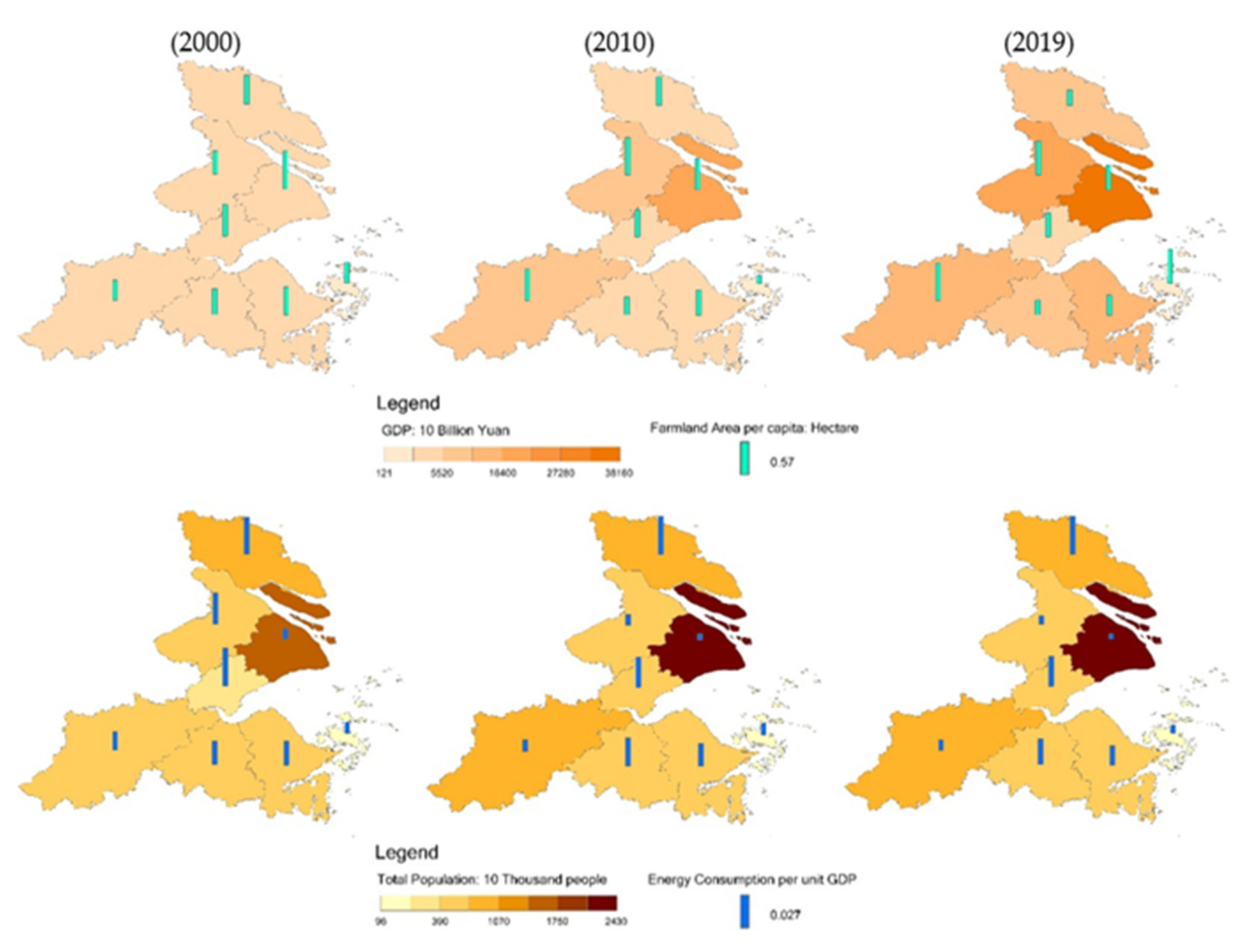
The Yangtze River Delta is an important area of socio-economic development in China. Based on the comparative analysis of total population, the gross domestic product (GDP), farmland area per capita and energy consumption per unit GPD during 1996–2019 (Figure 4), the conclusion are as follows. (1) The total population of eight cities grew rapidly. Due to the economic development center absorbing migration, the population of Shanghai has reached 24.28 million people. Due to the rapid utilization of land resources and the total population increasing, the farmland area per capita was decreasing. The top three cities were Suzhou, Shanghai and Hangzhou. (2) Driven by the national development planning and science technology support, the GPD of eight cities grew rapidly, with Nantong increasing from 72.06 billion Yuan to 897.2 billion Yuan and Zhoushan increasing from 12.2 billion Yuan to 125.0 billion Yuan. The average GDP ratio increased by 7–11 times, which was attributed to the National Planning of Regional Integrated Development in the Yangtze River Delta. (3) Because of the extensive development in the early stage, energy consumption per unit GPD increased quickly, thereby causing a frequent occurrence of the ecological and environmental problems. The average of energy consumption per unit GPD was 0.81 in 2000, and has decreased to 0.35. The health of the ecosystem was a prerequisite for socio-economic development.

Figure 4. Comprehensive analysis of total population, gross domestic product (GDP), farmland area per capita and energy consumption per unit GPD in the Yangtze River Delta.

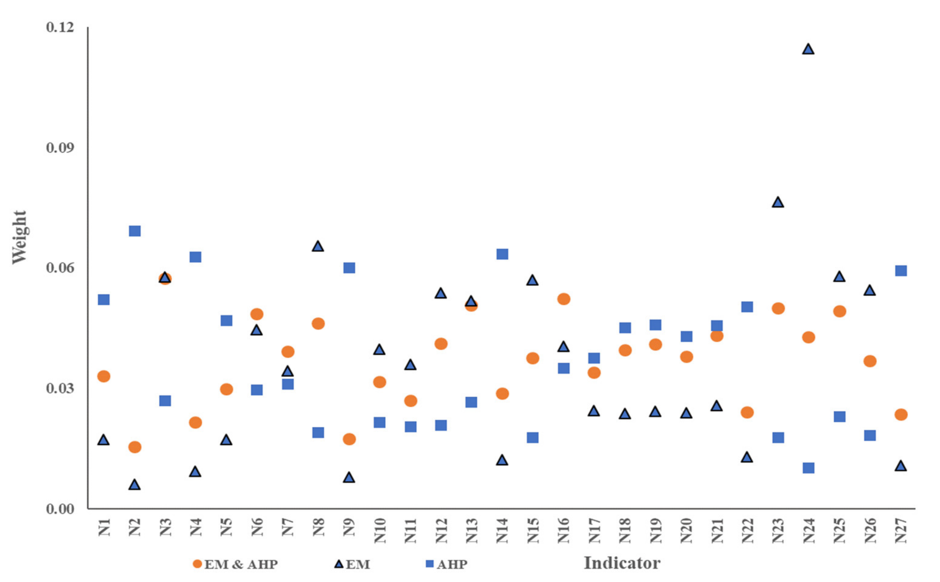
All third-class indicator data from eight cities during 1996–2019 were normalized based on the fuzzy quantification model [23]. In this study, we calculated the weight during 1996–2019 by using AHP and EM, respectively, and the final weight is the average of each year’s result (Figure 5). The largest weight indicator discovered using the EM method is the public budget expenditure (0.1146), but the largest one is found by using AHP method is construction area per capita (0.0692). In order to eliminate the shortcomings of subjective and objective calculation method, the indicator weight is calculated based. Table A1 in Appendix A shows the normalized indicator value of eight cities in 2019 and the final indicator’s weight.

Figure 5. Scatter diagram of the indicator weight of the ICC index system. Note: Data were calculated by AHP, EM and improved method. They are from Table A2 in Appendix A.

Based on the improved weight calculation method, the difference in each indicator is significantly revealed. The weight of fishery resources based on AHP is 0.0692 and the rank is 17, but it is 0.0577 based on the EM method and a rank of 5. This indicator is very important for current coastal city development. With the improved method in this study, the weight is 0.0573 and the rank is 1. The weight of industrial wastewater discharge based on AHP is 0.0296 and the rank is 16, and it is 0.0446 based on the EM method and a rank of 10. These two weights cannot reflect the importance of the ecological environment. Based on the improved method, the weight is updated to 0.0486 and the rank to 6.

4.1. ICC Evaluation Results Analysis

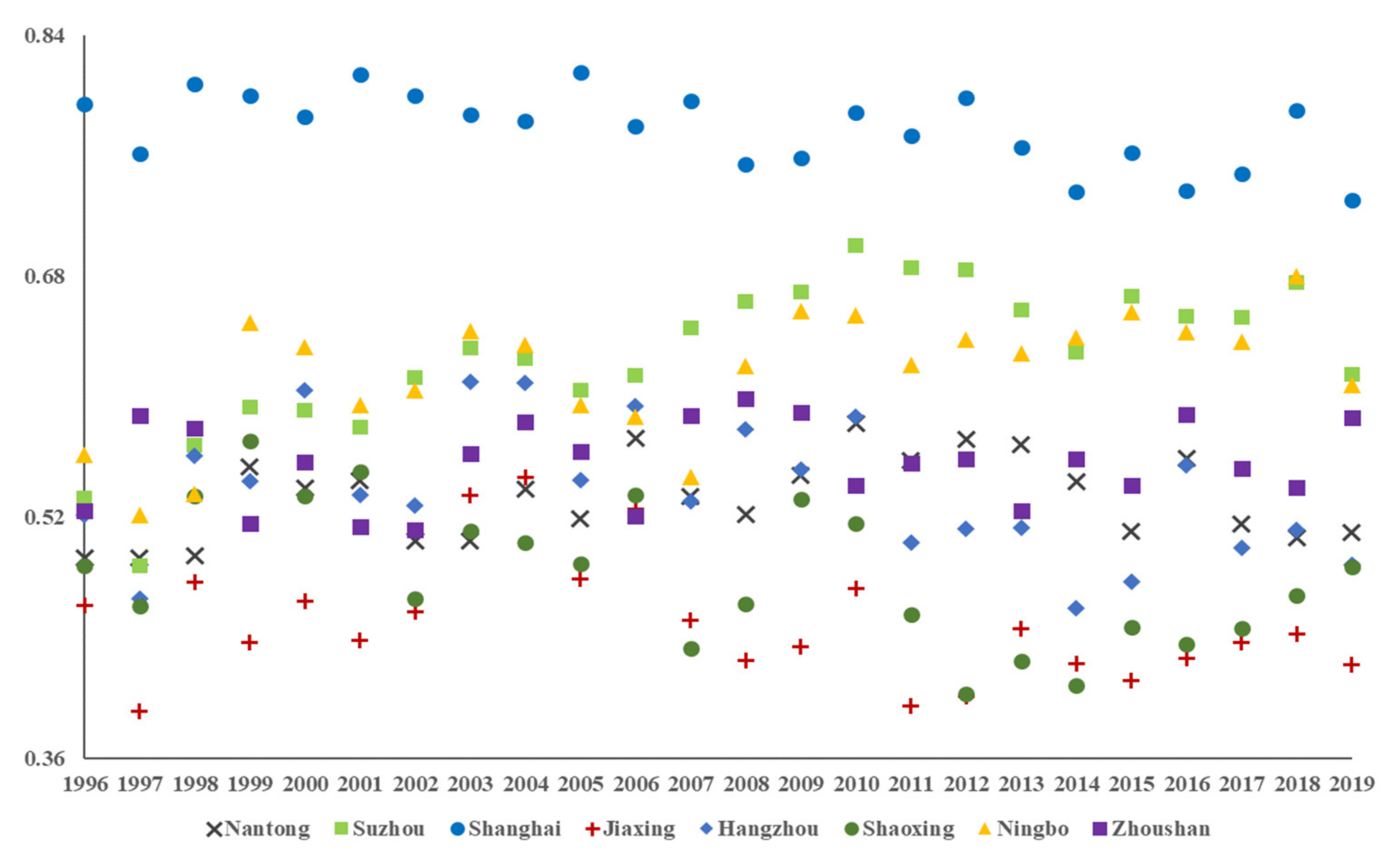
After the data normalization and weight calculation of third-class indicators, the ICC values of eight cities were calculated by using the state-space model [21]. Overall, the ICC of Shanghai is higher than other cities, with the highest value of 0.8154 in 2005. However, the ICC changing tendency of Shanghai was a fluctuating process during 1996–2019 (Figure 6), showing a downward tendency as a whole, which is due to the imbalance between natural ecological CC and socio-economic development.

Figure 6. Scatter diagram of ICC evaluation result of eight cities during 1996–2019. Note: Data were calculated by the space-state model. They are from Table A3 in Appendix A.

Based on the ICC changing tendency analysis of eight cities, Suzhou and Ningbo shows a relatively stable increasing tendency, and the largest value is 0.6758 and 0.6797 in 2018, respectively, in a same year. However, Nantong and Zhoushan presents a large volatility change. The ICC of Nantong increased 0.0603 from 2008 to 2010, but decreased 0.061 from 2012 to 2015. The ICC of Zhoushan increased to 0.0777 from 2006 to 2008, but decreased to 0.0716 from 1996 to 1998. The volatility change of ICC is caused by the imbalance between the demand of the socio-economic development and natural ecological CC, presenting the idea that humans are actively policy adjusting. The ICC of Jiaxing, Hangzhou and Shaoxing presented a very small change in volatility, which was decided by a comprehensive factor of the socio-economic development model, geographic location, species and quantity of natural resources, and so forth.

4.2. Indicator Data Estimation Result Analysis

Based on the grade ratio and validity requirement of the indicator evaluation data, the total number of prediction data is 10 years, from 2010 to 2019, which was satisfied with all indicators in the eight cities. Table A4 in Appendix A presents the grade ratio of indicator data in Nantong. From the proposed $GM\left(1,1\right)$ model, the grey development coefficient and grey control parameter of each indicator are as shown in Table A5 in Appendix A.

Based on the indicator data of Nantong during 2010–2019, the indicator estimation result from 2011 to 2019 is calculated by using the coefficient of the GM model. The average of the relative residual and deviation grade ratio of 27 indicators are calculated by using original data and estimated result. Figure 7 presents how all of the relative residual values are less than 0.1, but some values of the deviation grade ratio are more than 0.2. The indicator deviation grade ratio of industrial SO₂ emission, energy consumption per unit GPD, proportion of S and T personnel, actual utilized foreign investment and public budget expenditure are less than the requirement of the GM model. Although the values of these indicators are determined by the scale of socio-economic development, the relative residual of these indicators are satisfied with the model requirement. Thus, the accuracy of grey development coefficient and grey control parameter is suitable for indicator data estimation in the future year.

Figure 7. The radar diagram of average relative residual and deviation grade ratio of each indicator.

4.3. ICC Predication

4.3.1. Association Degree Calculation

In order to reflect the rank of ICC status and reduce calculation complexity, the association degree between ICC and indicator data was divided to three ranks in this study, which reflects high carrying capacity, middle carrying capacity and low carrying capacity. The association degree set is denoted as $\mu =\left[\begin{array}{ccc}{\mu }_1& {\mu }_2& {\mu }_3\end{array}\right]$.

Taking 1996 as the base year, the growth ratios of each third-class indicator data of eight cities were calculated during 1996–2019. To rescale the association degree into the interval of $\left[0,1\right]$, the coefficient of $d_0$ and $e_0$ are assigned as 0.5 and 0.2; however, no influence was found on the SPA calculation result. The association degree coefficient of eight cities is shown in Table 2.

Table 2. The association degree coefficient of evaluation years in this study.

City	μ1			μ2			μ3
	a	b	c	a	b	c	a	b	c
Nantong	0.5251	0.2835	0.1914	0.5152	0.2901	0.1947	0.5302	0.2801	0.1897
Suzhou	0.5257	0.2832	0.1912	0.5195	0.2869	0.1936	0.5237	0.2839	0.1924
Shanghai	0.5103	0.2929	0.1967	0.5106	0.2929	0.1966	0.5095	0.2937	0.1968
Jiaxing	0.5252	0.2831	0.1917	0.5167	0.2891	0.1943	0.5310	0.2798	0.1892
Hangzhou	0.5208	0.2863	0.1929	0.5125	0.2918	0.1957	0.5225	0.2853	0.1922
Shaoxing	0.5244	0.2841	0.1915	0.5160	0.2896	0.1943	0.5208	0.2859	0.1933
Ningbo	0.5290	0.2810	0.1899	0.5213	0.2863	0.1924	0.5216	0.2851	0.1933
Zhoushan	0.5280	0.2815	0.1905	0.5172	0.2887	0.1942	0.5339	0.2777	0.1884

Based on the third-class indicator prediction result of the eight cities from 2020 to 2030, the association degree of prediction years was calculated. Table 3 shows the association degree equation of eight cities in 2020.

Table 3. The association degree equation of eight cities in 2020.

City	Association-Degree	City	Association-Degree
Nantong	${\mu }_{2020}=0.5204+0.2865i+0.1931j$	Hangzhou	${\mu }_{2020}=0.5119+0.2918i+0.1963j$
Suzhou	${\mu }_{2020}=0.5217+0.2846i+0.1936j$	Shaoxing	${\mu }_{2020}=0.5019+0.2975i+0.2006j$
Shanghai	${\mu }_{2020}=0.5038+0.2966i+0.1996j$	Ningbo	${\mu }_{2020}=0.5075+0.2946i+0.1979j$
Jiaxing	${\mu }_{2020}=0.5080+0.2945i+0.1976j$	Zhoushan	${\mu }_{2020}=0.5163+0.2887i+0.1950j$

4.3.2. Ideal ICC Value Screening

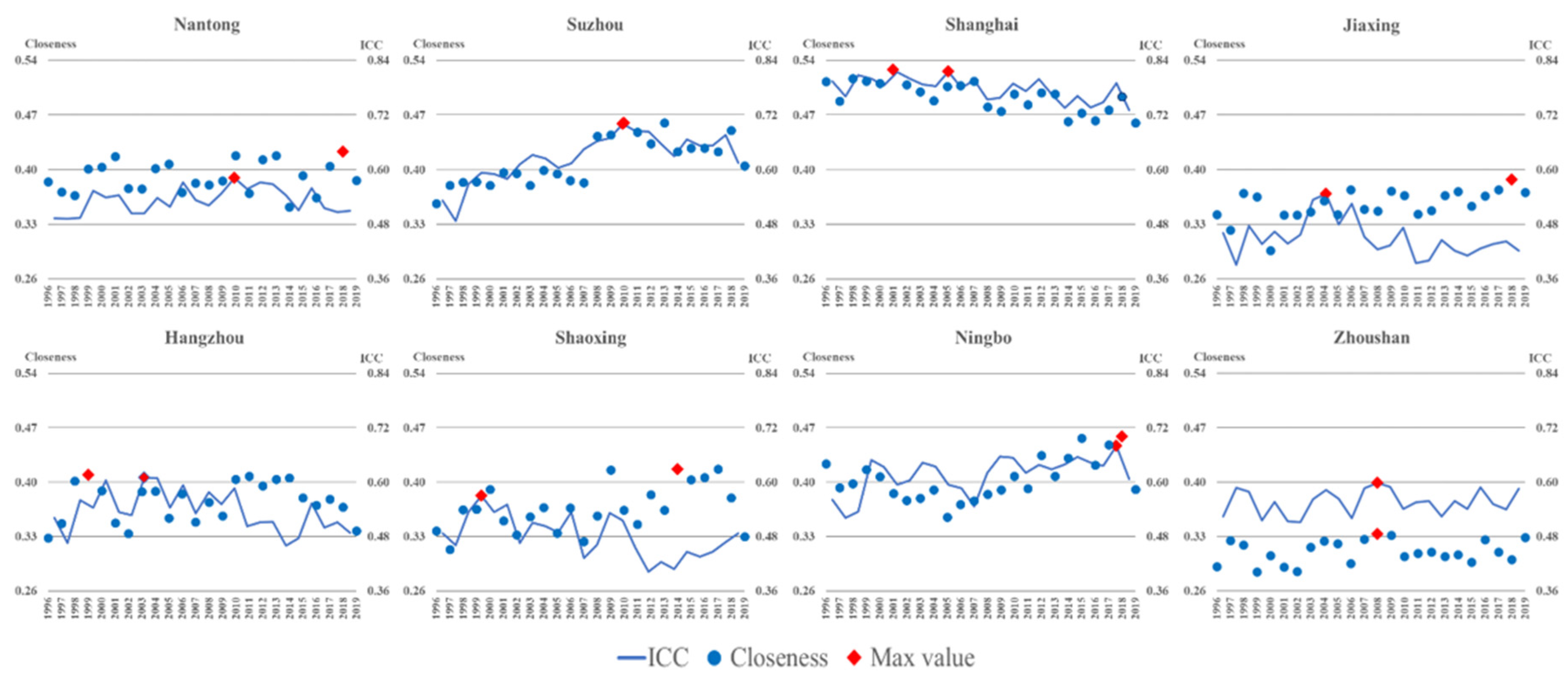
The closeness presents an order of coordination, that is, a collaborative relationship about each sub-system of ICC. Based on the normalized value and weight of the third-class indicator, the closeness parameter of eight cities were calculated. Figure 8 shows the closeness results of eight cities during 1996–2019. Overall, the closeness of Shanghai was higher than that of the other cities, but Zhoushan was the lowest one. This was due to the strong power of the socio-economic development scale and natural resource utilization in Shanghai, however, a downward tendency in volatility was found after 2008. On the contrary, the closeness of Zhoushan was lower than others because of the relative scarcity of the land resource area. With the land and marine coordinate exploitation, especially in fisher resource, the closeness of Zhoushan was slowly increased, and the largest value was 0.3329 in 2008.

Figure 8. Scatter diagram of closeness parameter of eight cities during 1996–2019. Note: Data were calculated by space-state model and TOPSIS model. They are from Table A3 and Table A5 in Appendix A.

Based on the maximum and minimum of each city’s closeness, the difference extent of Zhoushan and Nantong was smaller, which meant the coordination of ICC sub-system was keeping well in the socio-economic development progress. The difference in Suzhou, Shaoxing and Ningbo was up to 0.103, which was larger than the other cities. In social development, unscientific planning will certainly lead to a persistent coordination change in the ICC sub-system.

Comparing the ICC value with the closeness parameter, the following conclusions are as follows: First, the maximum of closeness value of Suzhou, Ningbo and Zhoushan appeared in 2010, 2018 and 2008, respectively, and the maximum of ICC value of these three cities also appeared in the same year. The ICC can reflect the summarize of each sub-system CC, and the coordination of the sub-system is the best state. Thus, the maximum ICC value is the optimal reference in Suzhou, Ningbo and Zhoushan.

Second, the ICC difference ratio between maximum value and optimal reference value in Shanghai was −0.17%, and the ratios in Nantong, Jiaxing, Hangzhou and Shaoxing were −14.90%, 23.51%, −1.20% and 39.60%, respectively. The year interval between the maximum value and optimal value of Shanghai was 4 years during 2001–2005, and a same interval in Hangzhou during 1999–2004. This interval is a relatively short period, and the ICC difference is relatively small, so that the maximum ICC can be the optimal reference value in Shanghai and Hangzhou. However, the ratio of other cities is more than 10%, and the interval is a long period. Thus, the optimal ICC reference result is the average between the maximum value and the optimal value in Nantong, Jiaxing and Shaoxing. Table 4 shows the optimal ICC value of eight cities for ICC prediction.

Table 4. The optimal ICC reference value of eight cities.

	Nantong	Suzhou	Shanghai	Jiaxing	Hangzhou	Shaoxing	Ningbo	Zhoushan
Ideal ICC value	0.5080	0.6575	0.7721	0.4320	0.5160	0.4477	0.6435	0.5919

4.3.3. ICC Prediction

Based on the association degree of evaluation years and prediction years, the IDC distance of each prediction year was calculated. Table 5 shows the three categories of IDC distance of Nantong during 2020–2030. With the increase in the prediction time, the association degree between current state and future decreases quickly, and a similar tendency is observed in all three categories of ICC, which reflects high CC, middle CC and low CC.

Table 5. The IDC distance of Nantong from 2020 to 2030.

	ρ1	ρ2	ρ3
2020	0.0059	0.0065	0.0122
2021	0.0069	0.0192	0.0014
2022	0.0220	0.0342	0.0158
2023	0.0397	0.0518	0.0335
2024	0.0601	0.0722	0.0539
2025	0.0834	0.0955	0.0773
2026	0.1099	0.1219	0.1038
2027	0.1397	0.1516	0.1336
2028	0.1730	0.1849	0.1670
2029	0.2102	0.2220	0.2042
2030	0.2514	0.2632	0.2454

Considering the optimal ICC reference value of eight cities (Table 4), the ICC prediction values were calculated. Table 6 shows the ICC predication result of eight cities during 2020–2030. On comparing with the ICC evaluation value, the following conclusions are as follows: First, the ICC prediction result of eight cities maintain a relatively small fluctuation during 2020–2030, which mainly relate to the indicator estimation result based on GM model. Second, a noticeable change of the prediction result is observed during 2020–2024 in eight cites; however, it is relatively smooth for a long time. Third, only the ICC prediction result of Shanghai and Ningbo is similar to the polynomial fitting curve based on the ICC result during 1996–2019; however, there is a large difference in the polynomial curve of other cities during 2020–2030. We will actively adjust the balance between the socio-economic development scale and the natural CC to keep a long-time sustainable development, so that the ICC tendency is relatively stable in a specific period. Thus, this improved prediction model is suitable for regional ICC prediction in the future, especially for a short period of 5–10 years, which can support the formulation of regional development strategies and validate the rationality of established goals.

Table 6. The ICC prediction result of eight cities during 2020–2030.

ICC′	Nantong	Suzhou	Shanghai	Jiaxing	Hangzhou	Shaoxing	Ningbo	Zhoushan
2020	0.5026	0.6700	0.7715	0.4297	0.5131	0.4942	0.6522	0.5912
2021	0.5300	0.6611	0.7708	0.4286	0.5106	0.4964	0.6559	0.6174
2022	0.5141	0.6613	0.7688	0.4408	0.5204	0.4852	0.6499	0.6006
2023	0.5118	0.6618	0.7694	0.4366	0.5188	0.4887	0.6419	0.5982
2024	0.5110	0.6620	0.7696	0.4345	0.5180	0.4899	0.6442	0.5974
2025	0.5105	0.6621	0.7697	0.4337	0.5176	0.4904	0.6452	0.5970
2026	0.5103	0.6622	0.7698	0.4333	0.5174	0.4907	0.6457	0.5967
2027	0.5101	0.6622	0.7698	0.4331	0.5173	0.4909	0.6461	0.5965
2028	0.5100	0.6622	0.7699	0.4329	0.5172	0.4910	0.6463	0.5964
2029	0.5099	0.6622	0.7699	0.4328	0.5171	0.4911	0.6465	0.5963
2030	0.5098	0.6623	0.7699	0.4327	0.5171	0.4911	0.6466	0.5963

5. Conclusions

It is an effective way to carry out the dynamic evaluation and prediction analysis of ICC, to solve the problem of regional coordinated development and ecological civilization health. From the indicator date estimation based on GM theory and the optimal ICC reference value screening based on TOPSIS theory, an improved approach of ICC prediction model by using SPA is proposed, which is validated by using the data of eight coastal cities during 1996–2019 in the Yangtze River Delta. The main conclusions are as follows.

(1).

We improved the calculation method of indicator weight based on the compressive AHP and EM models. The important indicator of fishery resource, proportion of S and T personnel, growth rate of GPD, actual utilized foreign investment and volume of port cargo handled are used to evaluate the ICC value of eight cities. The weight of fishery resource based on AHP is 0.0692 and the rank is 17, but it is 0.0577 based on EM and a rank of 5. With the improved method, the weight is 0.0573 and the rank is 1. On the contrary, the weight based on traditional relatively important indicator, such as construction area per capita, density of highway and population density, has been reduced. These new key indicators are consistent with the national development strategies, such as land and marine coordination, sound ecological environment, technology powers and foreign trade.

(2).

The ICC result of eight cities presented a tendency of first increasing, and then decreasing or tending to be relatively stable during 1996–2019. An upward tendency of ICC was noticed in Nantong and Suzhou, and the largest value was 0.5819 and 0.7002, respectively, which appeared in the same year 2010. With socio-economic development, the potential of the natural ecosystem was gradually excavated, especially in fishery resource, proportion of S and T investment and volume of port cargo handled. The largest ICC value of Shanghai and Hangzhou was 0.8154 and 0.6070, appeared in 2005 and 2003, respectively. Because of the earlier socio-economic development, the potential of natural ecosystem reached its limitation more quickly, we should thus discover more new resources and technology to support sustainable development. The ICC values of Jiaxing and Shaoxing were lower than others, and the largest value appeared earlier than 2005. The regional integrated and coordinated development was the best way to solve this bottleneck problem. Although the largest ICC of Zhoushan was 0.5982, lower than Shanghai or Hangzhou, and appeared in 2008, the range of the extent of change was relatively stable. This was due to the land resource area limitation, and the land and marine coordinate exploitation solved this insufficiency.

(3).

Compared with the traditional ICC prediction method, we improved the workflow by including indicator data estimation based on GM model, optimal ICC reference value screening based on TOPSIS and ICC prediction based on SPA. The average relative residuals of 27 indicators are all less than 0.1, which keep the accuracy of grey development coefficient and grey control parameter, so that the indicator estimation value during 2020–2030 can present the indicator changing tendency. The optimal ICC reference value, used in the SPA model, is the key to predict the ICC value. The maximum or last year’s ICC value is chosen, but it cannot reflect the natural ICC state. The closeness parameter is a suitable refence to screen the optimal value based on the TOPSIS model. The ICC prediction results of eight cities maintain a relatively small fluctuation during 2020–2030, and a high accuracy is observed for a short period of 5–10 years.

The ICC presents the comprehensive carrying capacity of each natural sub-system, which is a dynamic combination and influence each other. The simply mathematical method cannot reflect the internal relationship of the natural ecosystem. We proposed an improved approach to the ICC predication model by including the indicator weight, indicator data estimation and optimal ICC reference value screening. This can support the formulation of regional development strategies and validate the rationality of established development goals for government policymakers and stakeholders.