A Freight Transportation Network Model with a New Bundling Option

Abstract

A bundling option in a freight transportation network model enables a certain amount of goods to be sent after grouping them into a bundle. Usually, each bundle occupies the space of a unit good and/or can be transshipped using a more economical transportation mode, which results in reduced transportation costs and carbon emissions. As bundling and unbundling also incur costs, it is important to use the bundling option in an economical way. Several freight transportation network models were developed to find an optimal bundling strategy that minimizes the total cost. The existing models assume that bundling and unbundling can be performed at all nodes, including transshipping nodes. However, in many applications, goods are bundled at the supply node and are not unbundled until they arrive at the demand node. A new model, proposed herein, allows bundling only at the supply nodes and unbundling at the demand nodes. We investigated the complexity of the new model and developed a solution method. Furthermore, we analyzed how the total cost is affected by the new assumption.

1. Introduction

In a freight transportation network with a bundling option, a certain amount of goods after grouping them into a bundle at the cost of a unit good. In many applications, as this study will show, bundling reduces costs as each bundle occupies the space of a unit good. In other applications, bundling means transshipping goods using a more economical transportation mode. In both cases, bundling lowers not only transportation costs, but also carbon emissions by reducing vehicle mileage. Therefore, the bundling option enables the construction of a smart and sustainable freight transportation system. However, as bundling and unbundling also incur costs, an optimization model is required to minimize the total cost, including transporting, bundling, and unbundling costs.

Myung and Yu [1] addressed the freight transportation network problem with bundling option (FTNPB), which is a variant of the minimum-cost network flow problem. The original version of the FTNPB assumes that, initially, flows are not bundled at the supply node. Furthermore, it states that the flows delivered in a bundle at the demand node must be separated, or “unbundled”, and that bundling and unbundling can be performed at all nodes, including transshipping nodes. However, in many applications, locational restrictions exist on bundling and unbundling operations, where bundling is allowed only at the supply node and unbundling only at the demand node, for example. We refer to such a locational restriction as a “bundling and unbundling restriction” (hereafter referred to as a B/UB restriction). We also refer to the new version of the FTNPB with a B/UB restriction as the FTNPB-R. In this study, we focus on the FTNPB-R.

A representative application of the FTNPB is the problem of relocating empty foldable containers. Owing to imbalanced supply and demand of containers, repositioning empty containers is a key component in container transportation. Relocation is also an important issue in other fields, for example, the vehicle sharing field (Fanti et al. [2] and Zhang et al. [3]) and the medical field (Fanti et al. [4]). Several studies on empty container relocation have been published. Examples include research by Myung and Yu [1] and Myung et al. [5]. Most of the earlier studies are concerned with an unfolded container. After Konings and Thijs [6] and Konings [7] analyzed the potential cost savings of foldable containers, a variety of foldable container relocation models have been studied. As either four or six foldable containers can be folded to occupy the space of a single regular container, folding and unfolding can be represented as bundling and unbundling, and the FTNPB is applicable to foldable container relocation. Goh [8] shows that foldable containers contribute to carbon abatement. Shintani et al. [9] used restricted versions of the FTNPB to describe the problem of relocating empty containers in hinterland transportation, and Myung and Yu [1] generalized the model. All the models proposed by Shintani et al. [9] and Myung and Yu [1] assume that B/UB restrictions do not exist. However, in many applications, it does not appear practical for the containers transported from a supply node to a demand node to be unloaded for folding or unfolding at some intermediate nodes. Therefore, in this case, the FTNPB-R is preferable.

In addition to foldable container relocation, the FTNPB also has applications in multimodal freight transportation, as shown by Myung and Yu [1]. In this instance, goods are sent from manufacturers in a small carrier to the supply node and must be delivered to customers in a small carrier at the demand node. Shipping companies can use a large carrier to reduce transportation costs between supply and demand nodes, for which transshipping operations occur at both nodes. Bundling involves transshipping goods from a small carrier into a larger one, and the reverse in the case of unbundling. In this case, it is assumed that transshipping is allowed only at supply and demand nodes and not at intermediate nodes. Additionally, the FTNPB-R model is required.

The FTNPB is a single-commodity problem, but it has the characteristics of a two-commodity problem. A single-commodity problem can be solved in polynomial time (Ahuja et al. [10]) but a two-commodity network flow problem is NP-hard (Fortune et al. [11]). Myung [12] showed that when the underlying network has a star structure, similar to that proposed by Shintani et al. [9], the FTNPB can be solved in polynomial time. Meanwhile, Myung and Yu [1] showed that the FTNPB on an arbitrary network is NP-hard. Therefore, it is interesting to determine whether the B/UB restriction affects the computational complexity of the FTNPB. We show that the FTNPB-R can be transformed into the FTNPB on a bipartite network, and we analyze the complexity of the transformed problem.

This study can be summarized as follows. Firstly, we introduced an integer programming formulation for the FTNPB-R and analyzed the computational complexity of the problem. Secondly, we developed an efficient solution method for the FTNPB-R and performed intensive computing experiments to test our algorithm. We also provided computational results to analyze how B/UB restrictions affect the total cost. Thirdly, as performed by Myung and Yu [1] for the FTNPB, we considered the variable bundling model of the FTNPB-R, in which arbitrary numbers of flows can be bundled up to a given limit.

The remainder of this paper is organized as follows. In Section 2, we present an integer programming formulation for the FTNPB-R. In Section 3, we investigate the complexity of the problem and develop an efficient method for solving the proposed integer programming model. In Section 4, we consider the variable bundling version. The computational results are reported in Section 5, and concluding remarks are presented in Section 6.

2. Problem Description and Mathematical Formulation

In this section, we develop an integer programming formulation for the FTNPB-R. Given transportation network $G=\left(N,A\right)$, let $N_S\subseteq N$ be the set of supply nodes and $N_D\subseteq N$ be the set of demand nodes. Nodes in $N$, other than the supply and demand nodes, are transshipment nodes. Each arc corresponds to a transportation service and has an associated cost. Let $S_i$ denote the supply associated with the supply node $i$ and $D_j$ denote the demand associated with the demand node $j;$ we assume that ${{\displaystyle \sum }}_{i\in N_S}{S}_i={{\displaystyle \sum }}_{j\in N_D}{D}_j$. Similar to the FTNPB, the FTNPB-R assumes that $b$ flows are grouped in a single bundle, and that the transportation cost of one bundle on each arc is the same as that of a unit flow. The FTNPB-R aims to send flows from the supply nodes to satisfy the demands of the demand nodes at a minimum cost. We use the following notation to describe the cost coefficients.

$C_{ij}$: Unit transportation cost associated with arc (i, j).

$C_i^B$: Unit bundling cost at node i.

$C_i^U$: Unit unbundling cost at node i.

Unlike the FTNPB, the FTNPB-R assumes that once a flow starts from a supply node in a bundle, the flow to a demand node occurs under the same condition. Therefore, when we send flows from supply node $i$ to demand node $j$, regardless of whether the flows are bundled, we can minimize the transportation cost by sending them through the shortest cost path from node $i$ to node $j$. Let $C_{ij}^P$ be the sum of transportation costs of arcs in the shortest cost path from the supply node $i$ to the demand node $j$. Using the following additional notations as decision variables, we describe the problem in mathematical form.

$x_{ij}$: Number of flows transported unbundled from the supply node $i$ to the demand node $j$.

$y_{ij}$: Number of bundles transported from the supply node i to the demand node j.

The flows from the source node i to the demand node j are $x_{ij}+b{y}_{ij},$ and the total cost can be expressed as ${{\displaystyle \sum }}_{i\in N_S}{{\displaystyle \sum }}_{j\in N_D}\left\{C_{ij}^P{x}_{ij}+\left(C_{ij}^P+b{C}_i^B+b{C}_j^U\right)y_{ij}\right\}$. Note that the transportation costs of one bundle ($b$ flows) and a unit flow are identical, represented by $C_{ij}^P.$ When a bundle is sent, $b$ flows per bundle must be bundled and unbundled. The integer programming formulation for the FTNPB-R is as follows:

$$\left(\mathrm{P}\right) \mathrm{minimize} {\displaystyle \sum }_{i\in N_S}{\displaystyle \sum }_{j\in N_D}\left\{C_{ij}^P{x}_{ij}+\left(C_{ij}^P+b{C}_i^B+b{C}_j^U\right)y_{ij}\right\}$$

$$\mathrm{subject} \mathrm{to} {\displaystyle \sum }_{j\in N_D}\left(x_{ij}+b{y}_{ij}\right)=S_i\hspace{1em}\hspace{1em}\hspace{1em}\forall i\in N_S$$

(1)

$${\displaystyle \sum }_{i\in N_S}\left(x_{ij}+b{y}_{ij}\right)=D_j\hspace{1em}\hspace{1em}\hspace{1em}\forall j\in N_D$$

(2)

$$x_{ij},y_{ij}\ge 0 \mathrm{and} \mathrm{integer}\hspace{1em}\hspace{1em}\hspace{1em}\forall i\in N_S,j\in N_D$$

(3)

(P) can be viewed as a variant of the transportation problem, which is a minimum-cost flow problem in a bipartite network. Although the FTNPB-R is defined on an arbitrary network $G=\left(N,A\right)$, it can be transformed into a problem on a bipartite network through a B/UB restriction.

3. Problem Complexity and Solution Method

In this section, we study the computational complexity of (P) and demonstrate that (P) is NP-hard. For this purpose, we introduced the following NP-complete decision version of 3-EXACT COVER (X3C):

X3C INSTANCE: A family $F=\left\{S_1,\cdots ,S_n\right\}$ of three element subsets of $S=\left\{a_1,\cdots ,a_{3m}\right\}$.

QUESTION: Is there a subfamily of $m$ subsets that covers $S$?

Theorem 1.

(P) is NP-hard.

Proof. 

We demonstrate that X3C is reducible to the decision version of (P). Given an instance of X3C, an instance of (P) is associated with it using the following procedure. We constructed a bipartite transportation network with 3m + 1 supply nodes and $n$ demand nodes. Among the supply nodes, each of the 3m nodes correspond to each element in $S$ and the other node is a dummy node. Let $N_S^1=\left\{1,\cdots ,3m\right\}$ and $N_S=N_S^1\cup \left\{3m+1\right\}$. Each demand node corresponds to each element in $F,$ and let $N_D=\left\{1,\cdots ,n\right\}$. In the network, arc $\left(i, j\right)$ exists if $a_i\in S_j$ for each $i\in N_S^1$ and $j\in N_D$. In addition, there also exists an arc from a dummy supply node to every demand node, that is, $\left(3m+1, j\right)$ for each $j\in N_D$. We set $S_i=1$ for all $i=1,\cdots ,3m$, $S_{3m+1}=3\left(n-m\right)$, and $D_j=3$ for all $j\in N_D$. We assume that $b=3$. Set $C_{ij}=1$ for all arcs $\left(i,j\right)$. The answer to the X3C instance is yes if the associated (P) has a feasible solution with a cost of $3m+\left(n-m\right)$. □

Corollary 1.

The FTNPB on a bipartite network is NP-hard.

Proof. 

If a given transportation network is bipartite, the FTNPB also satisfies the B/UB restriction, because no transshipping node exists. Therefore, the FTNPB in a bipartite network can be described by (P), except that $C_{ij}^P$ is simply $C_{ij}$. □

Although the FTNPB on an arbitrary network is NP-hard (Myung and Yu [1]), it can be solved in polynomial time if the given network is a star network, as shown by Myung [12]. Therefore, Corollary 1 provides interesting information on the computational complexity of the FTNPB in another network with a special structure.

Hereafter, we develop a solution method for the integer programming problem (P). Although (P) is NP-hard like the FTNPB, it is expected to take less time to solve because the underlying network of (P) is a bipartite network. Through our computing experiments, the expectation was observed to be correct. However, it still took a considerable time to solve an extended model of (P); for example, the variable bundling model presented in Section 4. Therefore, we developed a heuristic for solving (P) that obtains near-optimal solutions within a reasonable time. The heuristic is based on the linear programming relaxation of (P), denoted by (LP), where the integrality condition in (3) is replaced by the non-negativity condition. We first show that (LP) can be transformed into a (Hitchcock) transportation problem, and thus it can be solved efficiently using a specialized transportation problem algorithm.

Lemma 1.

(LP) can be transformed into a transportation problem.

Proof. 

By replacing the term $b{y}_{ij}$ with $f_{ij}$, (LP) can be transformed into the following equivalent problem:

$$\left(\mathrm{LP}\right) \mathrm{minimize} {\displaystyle \sum }_{i\in N_S}{\displaystyle \sum }_{j\in N_D}\left\{C_{ij}^P{x}_{ij}+\left(\frac{1}{b}{C}_{ij}^P+C_i^B+C_j^U\right)f_{ij}\right\}$$

$$\mathrm{subject} \mathrm{to} {\displaystyle \sum }_{j\in N_D}\left(x_{ij}+f_{ij}\right)=S_i\hspace{1em}\hspace{1em}\hspace{1em}\forall i\in N_S$$

$${\displaystyle \sum }_{i\in N_S}\left(x_{ij}+f_{ij}\right)=D_j\hspace{1em}\hspace{1em}\hspace{1em}\forall j\in N_D$$

$$x_{ij},f_{ij}\ge 0\hspace{1em}\hspace{1em}\hspace{1em}\forall i\in N_S, j\in N_D$$

It is clear that either $x_{ij}$ or $f_{ij}$ have positive values. To minimize the objective function, we selected a variable with a smaller cost coefficient. We select $x_{ij}$, if $C_{ij}^P\le \frac{1}{b}{C}_{ij}^P+C_i^B+C_j^U$ and $f_{ij}$, otherwise. (LP) can then be transformed into the following transportation problem:

$$\left(\mathrm{TP}\right) \mathrm{minimize} {\displaystyle \sum }_{i\in N_S}{\displaystyle \sum }_{j\in N_D}min\left\{C_{ij}^P, \left(\frac{1}{b}{C}_{ij}^P+C_i^B+C_i^U\right)\right\}{r}_{ij}$$

$$\mathrm{subject} \mathrm{to} {\displaystyle \sum }_{j\in N_D}{r}_{ij}=S_{i\hspace{1em}\hspace{1em}\hspace{1em}} \forall i\in N_S$$

$${\displaystyle \sum }_{i\in N_S}{r}_{ij}=D_j\hspace{1em}\hspace{1em}\hspace{1em}\forall j\in N_D$$

$$r_{ij}\ge 0\hspace{1em}\hspace{1em}\hspace{1em}\forall i\in N_S, j\in N_D$$

where $r_{ij}$ is a substitution for either $x_{ij}$ or $f_{ij}$. □

Our algorithm first solves (LP) (via (TP)) and fixes the value of variable $y_{ij}$ using the optimal solution of (LP). If $y_{ij}$ satisfies the integrality for all $i\in N_S \mathrm{and} j\in N_D$, then all $x_{ij}$ and the optimal solution of (LP) are also optimal for (P). Otherwise, we round down every fractional $y_{ij}$ and set the integer value to the value of $y_{ij}$. Finally, we determine the remaining variables $x_{ij}$ by solving the following subproblem (SP) of (P):

$$\left(\mathrm{SP}\right) \mathrm{minimize} {\displaystyle \sum }_{i\in N_S}{\displaystyle \sum }_{j\in N_D}{C}_{ij}^P{x}_{ij}$$

$$\mathrm{subject} \mathrm{to} {\displaystyle \sum }_{j\in N_D}{x}_{ij}=S_i-{\displaystyle \sum }_{j\in N_D}b{y}_{ij}\hspace{1em}\hspace{1em}\hspace{1em}\forall i\in N_S$$

(4)

$${\displaystyle \sum }_{i\in N_S}{x}_{ij}=D_j-{\displaystyle \sum }_{i\in N_S}b{y}_{ij}\hspace{1em}\hspace{1em}\hspace{1em}\forall j\in N_D$$

(5)

$$x_{ij}\ge 0 \mathrm{and} \mathrm{integer}\hspace{1em}\hspace{1em}\hspace{1em}\forall i\in N_S, j\in N_D$$

(6)

(SP) is also a transportation problem that can be solved efficiently using a transportation problem algorithm.

4. Variable Bundling

Myung and Yu [1] considered the extended model of the FTNPB; they called it the FTNPB with variable bundling, where up to $b$ flows can be bundled. We considered the same extended version of the FTNPB-R, which we call the FTNPB-R with variable bundling. We developed a mathematical programming formulation for the extended model. Let the variables $y_{ij}^k$ for $2\le k\le b$ be the number of bundles, each of which groups $k$ flows and is transported from the supply node i to the demand node j. The FTNPB-R with variable bundling can then be formulated as follows:

$$\left(\mathrm{PV}\right) \mathrm{minimize} {\displaystyle \sum }_{i\in N_S}{\displaystyle \sum }_{j\in N_D}\left\{C_{ij}^P{x}_{ij}+\left(C_{ij}^P+2C_i^B+2C_j^U\right)y_{ij}^2+\cdots +\left(C_{ij}^P+b{C}_i^B+b{C}_j^U\right)y_{ij}^b\right\}$$

$$\mathrm{subject} \mathrm{to}{\displaystyle \sum }_{j\in N_D}\left(x_{ij}+2y_{ij}^2+\cdots +b{y}_{ij}^b\right)=S_i\hspace{1em}\hspace{1em}\hspace{1em}\forall i\in N_S$$

$${\displaystyle \sum }_{i\in N_S}\left(x_{ij}+2y_{ij}^2+\cdots +b{y}_{ij}^b\right)=D_j\hspace{1em}\hspace{1em}\hspace{1em}\forall j\in N_D$$

$$x_{ij},y_{ij}^k\ge 0 \mathrm{and} \mathrm{integer}\hspace{1em}\hspace{1em}\hspace{1em}\forall i\in N_S, j\in N_D, 2\le k\le b$$

A slight modification of our heuristic developed for solving (P) in Section 2 can also be applied to (PV). After solving the linear programming relaxation of (PV), denoted by (LPV), $y_{ij}^k$ is fixed with $2\le k\le b$ by truncating the fractional solution of (LPV), and the remaining $x_{ij}$ are determined through the following problem:

$$\left(\mathrm{SPV}\right) \mathrm{minimize} {\displaystyle \sum }_{i\in N_S}{\displaystyle \sum }_{j\in N_D}{C}_{ij}^P{x}_{ij}$$

$$\mathrm{subject} \mathrm{to} {\displaystyle \sum }_{j\in N_D}{x}_{ij}=S_i-{\displaystyle \sum }_{j\in N_D}\left(2y_{ij}^2+\cdots +b{y}_{ij}^b\right)\hspace{1em}\hspace{1em}\hspace{1em}\forall i\in N_S$$

$${\displaystyle \sum }_{i\in N_S}{x}_{ij}=D_j-{\displaystyle \sum }_{i\in N_S}\left(2y_{ij}^2+\cdots +b{y}_{ij}^b\right)\hspace{1em}\hspace{1em}\hspace{1em}\forall j\in N_D$$

$$x_{ij}\ge 0 \mathrm{and} \mathrm{integer}\hspace{1em}\hspace{1em}\hspace{1em}\forall i\in N_S, j\in N_D$$

Similar to (SP), (SPV) is a transportation problem that can be solved using an efficient transportation problem algorithm. Moreover, based on the following observation, we can also solve (LPV) using an efficient transportation problem algorithm.

Lemma 2.

(LPV) can be transformed into a transportation problem.

Proof. 

By replacing $k{y}_{ij}^k$ with $f_{ij}^k$ for $2\le k\le b$, (LPV) can be transformed into the following equivalent problem:

$$\left(\mathrm{LPV}\right) \mathrm{minimize} {\displaystyle \sum }_{i\in N_S}{\displaystyle \sum }_{j\in N_D}\left\{C_{ij}^P{x}_{ij}+\left(\frac{1}{2}{C}_{ij}^P+C_i^B+C_j^U\right)f_{ij}^2+\cdots +\left(\frac{1}{b}{C}_{ij}^P+C_i^B+C_j^U\right)f_{ij}^b\right\}$$

$$\mathrm{subject} \mathrm{to}{\displaystyle \sum }_{j\in N_D}\left(x_{ij}+f_{ij}^2+\cdots +f_{ij}^b\right)=S_i\hspace{1em}\hspace{1em}\hspace{1em}\forall i\in N_S$$

$${\displaystyle \sum }_{i\in N_S}\left(x_{ij}+f_{ij}^2+\cdots +f_{ij}^b\right)=D_j\hspace{1em}\hspace{1em}\hspace{1em}\forall j\in N_D$$

$$x_{ij},f_{ij}^k\ge 0\hspace{1em}\hspace{1em}\hspace{1em}\forall i\in N_S, j\in N_D, 2\le k\le b$$

As $\frac{1}{2}{C}_{ij}^P>\cdots >\frac{1}{b}{C}_{ij}^P$, either $x_{ij}$ or $f_{ij}^b$ can have positive values in an optimal solution. The best choice for minimizing the objective function is to select $x_{ij}$, if $C_{ij}^P\le \frac{1}{b}{C}_{ij}^P+C_i^B+C_j^U$ and $f_{ij}^b$, otherwise. The resultant problem is (TP), introduced in the proof of Lemma 1. □

Our heuristic fixes the values of the variables $y_{ij}^k$ for $2\le k\le b$, using the optimal solution of (LPV). For each fractional $y_{ij}^b$, we first set $y_{ij}^b=y_{ij}^b$; if there exists $k$ where $2\le k\le b-1$, $b\left(y_{ij}^b-y_{ij}^b\right)\ge k$, and $\frac{1}{k}{C}_{ij}^P+C_i^B+C_j^U<C_{ij}^P$, we choose the maximum $k$ and set $y_{ij}^k=1$. The remaining $y_{ij}^k$ variables are set to 0.

5. Computational Results

In this section, we report the results of the computational experiments to evaluate the performance of our two heuristics and to analyze how the B/UB restriction affects the total cost. We also conducted a sensitivity analysis on our proposed model to determine how the changes in cost parameters affect the total cost. For all tests, we used the same data instances that were generated by Myung and Yu [1] in their computational experiments for the model without the B/UB restriction for the following reasons. Firstly, the data instances were generated on various networks with different numbers of nodes and network densities (ratio of generated arcs to total number of possible arcs). Secondly, to analyze the effects of the B/UB restriction, our results must be compared with similar computational results for the FTNPB presented by Myung and Yu [1]. We used data instances with 30, 50, 100, 150, 200, and 300 nodes, and assumed that b = 4. All test runs were performed on a PC (2.9 GHz and 8G RAM).

5.1. Performance of Our Heuristic

For intensive testing, we classified the data instances into two groups. The first group included data instances with 30, 50, and 100 nodes, and the second group consisted of large problems with 150, 200, and 300 nodes. The computational results of the first and second groups are summarized in Table 1 and Table 2, respectively, and visualized using a graph in Figure 1. For each group of problems, we evaluated the performance of our two heuristics: one for the fixed bundling model and the other for the variable bundling model. In each table, we first reported the objective values obtained from the linear programming relaxations of two different bundling models: (LP) (z(LP)) and (LPV) (z(LPV)). As shown in Section 4, (z(LP)) and (z(LPV)) are equivalent. We then provided the objective value of our heuristic (z(H)) and the optimal objective value (z(P)) for the fixed bundling model, and the corresponding values z(HV) and z(PV) for the variable bundling model. We also reported the computation times for calculating $C_{ij}^P$ from each supply node to each demand node to perform our heuristic and to solve the integer programming model. We used the optimization software CPLEX 22.1 to solve both integer and linear programming problems.

Table 1. Computational results for small-sized problems.

No. of Nodes	Network Density	z(LP) (=z(LPV))	Fixed Bundling (4 Flows)			Variable Bundling (2, 3, 4 Flows)			Computation Time (Seconds)
			z(H)	z(P)	$\frac{\mathit{z}\left(\mathit{H}\right)}{\mathit{z}\left(\mathit{P}\right)}$	z(HV)	z(PV)	$\frac{\mathit{z}\left(\mathit{H}\mathit{V}\right)}{\mathit{z}\left(\mathit{P}\mathit{V}\right)}$	${\mathit{C}}_{\mathit{i}\mathit{j}}^{\mathit{P}}$	Fixed Bundling		Variable Bundling
										H	P	HV	PV
30	0.2	38,549.5	42,539.0	41,601.9	1.02	40,706.0	39,962.1	1.02	0.040	0.016	0.140	0.015	0.922
		47,824.9	54,648.8	50,349.3	1.09	50,560.7	49,463.0	1.02	0.047	0.016	0.031	0.016	0.141
		43,534.2	47,719.7	46,425.8	1.03	45,825.9	45,021.2	1.02	0.041	0.015	0.031	0.016	0.219
		43,587.3	47,666.3	46,574.2	1.02	45,633.4	45,063.5	1.01	0.041	0.000	0.156	0.016	0.203
		52,826.2	56,334.6	55,617.7	1.01	54,618.6	54,229.6	1.01	0.052	0.000	0.172	0.016	0.203
	0.35	38,696.8	43,149.5	41,521.0	1.04	40,792.1	40,114.5	1.02	0.057	0.016	0.062	0.015	0.313
		38,823.8	44,551.0	41,707.9	1.07	40,722.0	39,944.5	1.02	0.061	0.015	0.157	0.015	0.281
		35,866.6	40,062.2	38,115.4	1.05	37,577.8	37,010.0	1.02	0.059	0.000	0.016	0.015	0.094
		50,049.2	53,963.7	52,638.6	1.03	51,701.1	51,221.5	1.01	0.045	0.015	0.062	0.015	0.110
		55,603.9	60,421.6	58,252.0	1.04	57,348.5	56,787.5	1.01	0.081	0.000	0.047	0.016	0.532
	0.5	43,031.2	47,271.1	45,090.2	1.05	44,671.6	44,071.4	1.01	0.070	0.016	0.187	0.000	0.125
		49,047.1	53,341.2	51,461.8	1.04	50,919.7	50,119.6	1.02	0.069	0.016	0.031	0.016	0.922
		38,438.8	41,805.1	40,575.1	1.03	40,108.8	39,449.0	1.02	0.077	0.015	0.031	0.015	0.204
		35,062.6	39,249.0	37,650.1	1.04	36,598.9	36,079.9	1.01	0.072	0.015	0.047	0.000	0.563
		40,583.1	44,910.4	42,888.7	1.05	42,182.9	41,614.5	1.01	0.066	0.000	0.078	0.015	0.047
50	0.2	65,654.5	72,172.3	70,076.1	1.03	68,339.1	67,642.0	1.01	0.173	0.015	0.078	0.016	2.297
		83,393.9	90,722.6	87,804.1	1.03	86,808.7	85,706.0	1.01	0.152	0.031	0.313	0.032	3.422
		70,942.3	78,581.1	75,902.0	1.04	74,380.0	73,303.8	1.01	0.225	0.031	0.906	0.015	1.656
		73,521.7	85,272.2	78,470.3	1.09	77,313.7	75,510.1	1.02	0.163	0.016	0.172	0.031	9.609
		62,195.5	69,916.0	66,989.6	1.04	64,856.0	64,102.1	1.01	0.193	0.032	0.484	0.015	1.750
	0.35	72,482.7	78,083.1	76,479.0	1.02	75,419.6	74,381.0	1.01	0.280	0.016	0.062	0.032	1.922
		76,501.8	82,677.1	79,786.8	1.04	79,333.6	78,298.4	1.01	0.248	0.016	0.219	0.015	4.750
		59,078.6	64,856.8	62,615.7	1.04	61,520.2	60,565.3	1.02	0.277	0.015	0.594	0.016	0.094
		66,049.0	71,739.3	69,624.9	1.03	68,850.5	67,677.9	1.02	0.259	0.000	0.109	0.016	0.312
		76,655.7	84,447.3	80,168.9	1.05	79,455.8	78,386.6	1.01	0.245	0.015	0.531	0.016	0.344
	0.5	66,734.2	73,623.3	70,021.4	1.05	69,737.5	68,367.6	1.02	0.356	0.015	0.047	0.016	2.641
		61,783.8	68,200.9	64,947.6	1.05	64,280.9	63,236.6	1.02	0.316	0.016	0.094	0.016	3.657
		65,038.7	71,631.1	68,602.4	1.04	68,171.1	66,582.8	1.02	0.320	0.016	0.094	0.016	0.359
		60,479.2	65,102.8	63,433.6	1.03	62,707.7	62,178.3	1.01	0.311	0.015	0.094	0.016	3.454
		61,454.2	67,887.9	65,143.4	1.04	64,547.9	63,050.1	1.02	0.329	0.000	0.235	0.015	0.218
100	0.2	146,960.1	164,015.2	156,708.2	1.05	153,541.8	150,929.9	1.02	1.210	0.047	1.734	0.078	12.796
		139,430.4	152,570.0	147,260.6	1.04	144,612.9	142,853.9	1.01	1.490	0.047	0.656	0.047	9.875
		145,488.5	159,903.8	152,864.1	1.05	152,069.9	148,858.2	1.02	1.621	0.047	0.672	0.047	55.578
		123,636.1	136,175.0	130,979.2	1.04	129,559.9	127,267.9	1.02	1.366	0.047	0.391	0.047	9.453
		119,307.7	134,006.3	127,662.3	1.05	124,966.4	122,427.7	1.02	1.445	0.047	0.125	0.047	7.688
	0.35	134,472.5	148,102.7	142,055.3	1.04	139,734.9	137,366.7	1.02	1.883	0.062	1.703	0.047	9.922
		122,559.9	133,704.0	129,525.1	1.03	127,554.3	125,828.0	1.01	2.244	0.047	0.422	0.047	19.125
		118,575.4	132,031.8	124,750.1	1.06	123,753.5	121,430.6	1.02	2.160	0.047	0.688	0.047	21.907
		130,914.7	143,417.9	137,824.0	1.04	136,181.9	134,124.9	1.02	1.944	0.047	0.640	0.047	21.046
		125,046.0	137,495.1	131,992.0	1.04	130,436.7	127,882.4	1.02	2.126	0.031	4.657	0.046	5.297
	0.5	146,731.0	158,146.4	152,674.0	1.04	151,804.5	149,469.8	1.02	2.330	0.047	2.047	0.062	16.265
		122,944.1	138,228.5	129,992.6	1.06	129,351.5	126,177.7	1.03	2.524	0.047	2.329	0.062	12.078
		136,517.8	148,486.0	143,227.9	1.04	141,608.0	139,609.2	1.01	2.548	0.047	2.093	0.063	13.469
		118,029.5	129,556.4	125,118.5	1.04	123,180.7	120,869.9	1.02	2.820	0.047	0.313	0.062	9.078
		140,466.3	154,376.5	147,246.7	1.05	146,390.1	143,179.2	1.02	3.112	0.047	0.375	0.047	>200.0

Table 2. Computational results for large-sized problems.

No. of Nodes	Network Density	z(LP) (=z(LPV))	Fixed Bundling (4 Flows)			Variable Bundling (2, 3, 4 Flows)			Computation Time (Seconds)
			z(H)	z(P)	$\frac{\mathit{z}\left(\mathit{H}\right)}{\mathit{z}\left(\mathit{P}\right)}$	z(HV)	z(PV)	$\frac{\mathit{z}\left(\mathit{H}\mathit{V}\right)}{\mathit{z}\left(\mathit{P}\mathit{V}\right)}$	${\mathit{C}}_{\mathit{i}\mathit{j}}^{\mathit{P}}$	Fixed Bundling		Variable Bundling
										H	P	HV	PV
150	0.2	186,021.5	204,181.1	197,090.8	1.04	194,335.7	190,779.7	1.02	4.712	0.094	4.969	0.125	118.766
		188,070.4	208,907.5	198,984.1	1.05	195,516.2	192,528.2	1.02	4.964	0.078	0.641	0.109	141.703
		186,269.4	205,067.3	196,351.6	1.04	194,197.6	190,906.1 *	1.02	5.228	0.078	7.094	0.110	>200.0
		206,545.3	223,887.6	215,596.7	1.04	214,162.7	210,652.5	1.02	4.416	0.094	7.390	0.109	21.204
		212,834.5	230,929.9	223,722.4	1.03	220,362.9	217,391.8	1.01	4.285	0.078	1.281	0.110	75.844
	0.35	189,241.8	211,102.6	201,005.8	1.05	197,121.9	193,543.3 *	1.02	7.584	0.094	3.672	0.109	>200.0
		178,520.3	196,661.3	187,720.7	1.05	185,855.2	183,075.6	1.02	6.879	0.094	4.844	0.125	56.578
		184,497.0	203,573.0	193,797.2	1.05	192,182.3	188,732.3	1.02	7.234	0.094	0.875	0.125	45.563
		207,419.5	227,116.2	216,735.3	1.05	215,632.5	211,834.1 *	1.02	8.221	0.094	5.657	0.125	>200.0
		204,764.9	222,671.6	215,092.5	1.04	212,387.1	209,213.9	1.02	6.344	0.093	7.313	0.109	90.047
	0.5	197,161.2	215,351.0	206,805.7	1.04	204,896.9	201,486.8	1.02	8.728	0.093	1.641	0.125	116.718
		210,401.5	233,013.5	221,104.5	1.05	219,275.0	215,081.3 *	1.02	10.717	0.094	5.343	0.125	>200.0
		194,887.8	211,789.2	203,918.5	1.04	202,195.5	199,057.0	1.02	9.034	0.094	5.078	0.125	33.562
		186,103.7	203,894.8	195,185.6	1.04	193,597.0	190,209.0	1.02	9.803	0.094	0.640	0.125	145.203
		187,789.4	204,577.5	196,484.6	1.04	195,152.1	191,703.6	1.02	9.638	0.109	4.984	0.125	21.406
200	0.2	265,694.2	293,003.9	278,242.9	1.05	276,052.6	271,971.4	1.02	12.410	0.140	7.922	0.188	123.297
		266,388.3	291,343.4	279,358.2	1.04	276,870.0	273,194.1*	1.01	11.664	0.140	18.468	0.187	>200.0
		248,625.7	273,959.3	261,703.3	1.05	258,930.9	254,429.8	1.02	10.829	0.125	0.641	0.188	89.141
		268,625.2	294,868.9	282,156.2	1.05	278,275.1	275,047.2	1.01	10.607	0.141	5.563	0.188	196.234
		255,943.2	278,715.7	269,754.2	1.03	266,170.3	261,899.1	1.02	12.082	0.125	10.735	0.188	174.531
	0.35	241,651.2	267,602.9	255,854.2	1.05	251,881.6	248,194.0 *	1.01	17.203	0.157	11.203	0.203	>200.0
		274,468.4	301,392.9	288,321.0	1.05	286,237.9	280,967.8	1.02	14.427	0.156	14.312	0.203	162.766
		227,371.3	250,405.0	239,909.0	1.04	237,649.8	233,377.8 *	1.02	17.032	0.157	1.516	0.203	>200.0
		233,471.7	258,764.2	247,295.5	1.05	243,761.9	239,771.0 *	1.02	17.494	0.156	10.640	0.219	>200.0
		241,197.5	264,796.7	254,017.2	1.04	251,706.0	247,170.7	1.02	16.763	0.156	12.562	0.203	128.531
	0.5	239,972.6	266,232.1	253,593.7	1.05	251,442.3	246,094.4	1.02	21.883	0.172	9.063	0.203	162.250
		249,999.4	274,186.4	262,683.9	1.04	260,445.8	255,702.6 *	1.02	23.178	0.156	25.765	0.219	>200.0
		278,675.3	304,443.6	292,660.9	1.04	289,547.9	284,612.7	1.02	24.684	0.157	10.828	0.219	127.688
		227,237.9	249,030.6	239,973.2	1.04	236,377.7	232,500.0 *	1.02	21.410	0.172	5.938	0.250	>200.0
		254,442.1	277,356.8	267,816.0	1.04	265,929.7	260,642.1 *	1.02	20.238	0.156	17.922	0.218	>200.0
300	0.2	371,125.3	405,564.8	390,230.0	1.04	386,303.6	379,983.8 *	1.02	37.315	0.344	6.421	0.438	>200.0
		342,360.5	377,712.9	361,157.6	1.05	358,140.1	351,449.3	1.02	37.939	0.344	3.204	0.438	125.703
		344,723.9	381,496.4	363,880.3	1.05	360,203.9	354,247.7	1.02	39.551	0.344	6.937	0.453	157.984
		389,669.2	429,196.4	410,803.9	1.04	406,603.1	399,348.4	1.02	41.357	0.329	14.391	0.438	195.078
		377,427.3	412,750.1	397,185.5	1.04	392,556.2	386,124.4	1.02	36.834	0.360	14.328	0.453	143.375
	0.35	343,722.0	376,945.2	361,726.6	1.04	359,051.1	352,210.5	1.02	58.442	0.375	4.875	0.485	83.031
		349,822.5	381,646.7	367,922.9	1.04	364,278.9	358,513.1	1.02	56.283	0.406	16.985	0.484	196.140
		351,332.3	388,453.7	370,903.1	1.05	365,432.9	359,823.9	1.02	57.514	0.375	18.703	0.469	98.829
		382,843.8	415,349.7	401,904.0	1.03	397,551.3	391,594.8	1.02	53.727	0.406	30.703	0.500	100.547
		355,320.6	386,656.1	373,225.0	1.04	369,290.6	364,022.3	1.01	59.228	0.375	2.735	0.468	155.594
	0.5	388,961.1	424,683.6	407,933.9	1.04	403,916.8	396,804.5 *	1.02	69.960	0.375	21.047	0.500	>200.0
		379,047.1	418,412.8	398,560.6	1.05	394,950.3	387,871.5	1.02	83.034	0.375	7.312	0.500	145.656
		391,175.6	424,843.9	409,062.4	1.04	406,694.3	399,240.7	1.02	81.193	0.391	4.547	0.484	100.062
		353,861.8	388,483.2	372,150.8	1.04	369,322.6	361,983.0	1.02	77.186	0.375	12.656	0.500	196.875
		361,084.0	394,074.2	377,812.9	1.04	376,775.0	369,063.3	1.02	77.923	0.422	1.938	0.469	96.250

* Best solution obtained within the time limit.

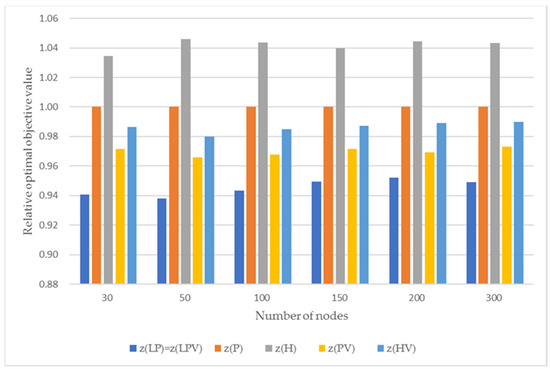
Figure 1. Graphic visualization of computational results.

The results indicate that our two heuristics find near-optimal solutions for fairly large problems within a reasonable timeframe. Interestingly, the heuristic for the variable bundling model performs better than that for the fixed bundling case. The average ratios of z(HV) to z(PV) were within 2 %, whereas those of z(H) to z(P) were within 5%. We provided the computation times for calculating $C_{ij}^P$ separately to clearly compare the times needed to obtain heuristic and integer optimal solutions. As expected, for the fixed bundling case, the integer optimal solution could be obtained in a relatively short time, even for large problems. These times were remarkably smaller than that for the FTNPB presented by Myung and Yu [1]. This can be explained by the fact that the new model can be transformed into the FTNPB in a simple bipartite network. However, for the variable bundling case, the integer programming solver incurred considerable time finding an exact solution and exceeded the time limit of 200 s for many large-sized problems. However, our two heuristics solved large-sized problems within a second, even for the variable bundling case.

5.2. Effects of Bundling and Locational Restriction

Myung and Yu [1] compared the total costs of three FTNPB models to investigate the effects of bundling: one with fixed bundling, one with variable bundling, and one without bundling. They found that bundling saves the total cost considerably, but the additional cost saving by variable bundling is not significant. The same experiments were conducted using the same three FTNPB-R models. We also compared our results with those of Myung and Yu [1] to analyze how the B/UB restriction affects the total cost. The results presented in Table 3 imply that the effects of different bundling strategies are almost the same between the two models with and without the B/UB restriction, and the restriction does not increase the total cost significantly.

Table 3. Effects of different bundling strategies and B/UB restriction.

No. of Nodes	Network Density	No Bundling (a)	FTNPB (without B\UB Restriction)				FTNPB-R (with B\UB Restriction)
			Fixed Bundling (b)	(b/a)	Variable Bundling (c)	(c/a)	Fixed Bundling (d)	(d/a)	Variable Bundling (e)	(e/a)
50	0.2	150,634.1	69,505.2	0.46	67,626.6	0.45	70,076.1	0.47	67,642.0	0.45
		183,959.8	86,960.0	0.47	85,523.1	0.46	87,804.1	0.48	85,706.0	0.47
		164,349.2	74,860.5	0.46	73,152.1	0.45	75,902.0	0.46	73,304.2	0.45
		187,986.8	77,555.2	0.41	75,366.9	0.40	78,470.3	0.42	75,510.1	0.40
		130,453.8	65,804.1	0.50	64,102.1	0.49	66,989.6	0.51	64,102.1	0.49
	0.35	136,158.9	76,056.8	0.56	74,381.0	0.55	76,479.0	0.56	74,381.0	0.55
		147,811.2	79,342.3	0.54	78,298.4	0.53	79,786.8	0.54	78,298.4	0.53
		129,450.3	62,021.5	0.48	60,565.3	0.47	62,615.7	0.48	60,565.3	0.47
		138,983.9	69,001.4	0.50	67,677.9	0.49	69,624.9	0.50	67,677.9	0.49
		151,634.9	79,964.8	0.53	78,386.6	0.52	80,168.9	0.53	78,386.7	0.52
	0.5	139,196.7	69,601.6	0.50	68,367.6	0.49	70,021.4	0.50	68,369.3	0.49
		128,955.2	64,577.6	0.50	63,236.6	0.49	64,947.6	0.50	63,236.6	0.49
		131,510.8	68,020.0	0.52	66,582.8	0.51	68,602.4	0.52	66,582.8	0.51
		120,749.0	63,244.5	0.52	62,175.5	0.51	63,433.6	0.53	62,178.3	0.51
		130,884.8	64,568.0	0.49	63,050.1	0.48	65,143.4	0.50	63,050.1	0.48

5.3. Sensitivity Analysis on Cost Parameters

We also conducted a sensitivity analysis to show how changes in transportation cost and folding/unfolding cost affect the total cost. As shown in Table 4 and visualized in Figure 2, bundling mitigates the increase in transportation costs. The same phenomenon was observed when the folding/unfolding cost decreased, as summarized in Table 5.

Table 4. Sensitivity analysis on the increases of transportation cost.

No. of Nodes	Network Density	Original Data (a)	10% Increase		20% Increase		30% Increase		40% Increase
			(b)	(c)	(b)	(c)	(b)	(c)	(b)	(c)
(No Bundling Case)
50	0.2	150,634.10	165,697.50	10.00%	180,760.90	20.00%	195,824.30	30.00%	210,887.70	40.00%
		183,959.80	202,355.70	10.00%	220,751.70	20.00%	239,147.70	30.00%	257,543.70	40.00%
		164,349.20	180,784.10	10.00%	197,219.00	20.00%	213,654.00	30.00%	230,088.90	40.00%
		187,986.80	206,785.50	10.00%	225,584.20	20.00%	244,382.90	30.00%	263,181.60	40.00%
		130,453.80	143,499.20	10.00%	156,544.60	20.00%	169,590.00	30.00%	182,635.40	40.00%
	0.35	136,158.90	149,774.80	10.00%	163,390.70	20.00%	177,006.60	30.00%	190,622.40	40.00%
		147,811.20	162,592.30	10.00%	177,373.40	20.00%	192,154.60	30.00%	206,935.70	40.00%
		129,450.30	142,395.30	10.00%	155,340.30	20.00%	168,285.40	30.00%	181,230.40	40.00%
		138,983.90	152,882.30	10.00%	166,780.70	20.00%	180,679.10	30.00%	194,577.50	40.00%
		151,634.90	166,798.40	10.00%	181,961.90	20.00%	197,125.30	30.00%	212,288.80	40.00%
	0.5	139,196.70	153,116.40	10.00%	167,036.10	20.00%	180,955.70	30.00%	194,875.40	40.00%
		128,955.20	141,850.70	10.00%	154,746.20	20.00%	167,641.70	30.00%	180,537.20	40.00%
		131,510.80	144,661.90	10.00%	157,813.00	20.00%	170,964.00	30.00%	184,115.10	40.00%
		120,749.00	132,823.90	10.00%	144,898.80	20.00%	156,973.70	30.00%	169,048.60	40.00%
		130,884.80	143,973.30	10.00%	157,061.80	20.00%	170,150.30	30.00%	183,238.80	40.00%
(Fixed bundling case)
50	0.2	70,076.10	74,442.50	6.20%	78,808.90	12.50%	83,175.30	18.70%	87,541.80	24.90%
		87,804.10	93,030.90	6.00%	98,257.70	11.90%	103,484.50	17.90%	108,711.30	23.80%
		75,902.00	80,677.40	6.30%	85,448.10	12.60%	90,218.80	18.90%	94,989.40	25.10%
		78,470.30	83,854.50	6.90%	89,238.70	13.70%	94,623.00	20.60%	100,007.20	27.40%
		66,989.60	70,892.10	5.80%	74,794.70	11.70%	78,697.20	17.50%	82,599.80	23.30%
	0.35	76,479.00	80,515.80	5.30%	84,552.50	10.60%	88,589.20	15.80%	92,625.90	21.10%
		79,786.80	84,002.20	5.30%	88,217.70	10.60%	92,433.20	15.90%	96,648.70	21.10%
		62,615.70	66,350.50	6.00%	70,085.20	11.90%	73,820.00	17.90%	77,554.80	23.90%
		69,624.90	73,651.40	5.80%	77,677.90	11.60%	81,704.30	17.30%	85,730.80	23.10%
		80,168.90	84,509.00	5.40%	88,849.00	10.80%	93,189.10	16.20%	97,529.20	21.70%
	0.5	70,021.40	74,003.20	5.70%	77,984.90	11.40%	81,966.70	17.10%	85,948.40	22.70%
		64,947.60	68,609.10	5.60%	72,270.70	11.30%	75,932.30	16.90%	79,593.80	22.60%
		68,602.40	72,415.00	5.60%	76,227.70	11.10%	80,040.30	16.70%	83,852.90	22.20%
		63,433.60	66,910.90	5.50%	70,388.30	11.00%	73,865.60	16.40%	77,343.00	21.90%
		65,143.40	68,929.70	5.80%	72,716.00	11.60%	76,502.40	17.40%	80,288.70	23.20%
$(\mathrm{c}) = \frac{\left(\mathrm{b}\right) - \left(\mathrm{a}\right)}{\left(\mathrm{a}\right)} \times 100(\%)$

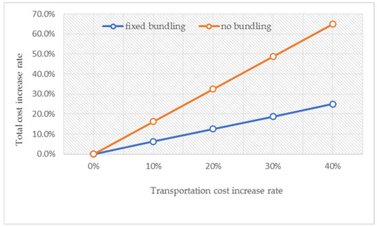
Figure 2. Sensitivity analysis on the increase in transportation cost (network density = 0.2).

Table 5. Sensitivity analysis on the decreases in folding and unfolding cost.

No. of Nodes	Network Density	Original Data (a)	10% Decrease		20% Decrease		30% Decrease		40% Decrease
			(b)	(c)	(b)	(c)	(b)	(c)	(b)	(c)
50	0.2	70,076.1	64,080.1	8.6%	59,836.1	14.6%	55,876.1	20.3%	52,248.1	25.4%
		87,804.1	84,264.1	4.0%	80,736.1	8.0%	76,732.1	12.6%	73,197.0	16.6%
		75,902.0	73,074.0	3.7%	70,074.7	7.7%	67,110.7	11.6%	64,464.7	15.1%
		78,470.3	75,994.3	3.2%	73,246.3	6.7%	70,838.3	9.7%	68,390.3	12.8%
		66,989.6	64,173.6	4.2%	61,229.6	8.6%	58,369.6	12.9%	55,509.6	17.1%
	0.35	76,479.0	72,691.0	5.0%	69,055.0	9.7%	65,391.0	14.5%	61,667.0	19.4%
		79,786.8	75,930.8	4.8%	72,242.8	9.5%	68,294.2	14.4%	64,274.2	19.4%
		62,615.7	60,115.7	4.0%	57,483.7	8.2%	54,847.7	12.4%	52,191.7	16.6%
		69,624.9	66,588.9	4.4%	63,692.9	8.5%	60,516.9	13.1%	57,592.9	17.3%
		80,168.9	76,416.9	4.7%	72,520.9	9.5%	68,912.9	14.0%	65,040.9	18.9%
	0.5	70,021.4	66,949.4	4.4%	63,785.4	8.9%	60,697.4	13.3%	57,521.4	17.9%
		64,947.6	61,987.6	4.6%	59,095.6	9.0%	56,227.6	13.4%	53,247.6	18.0%
		68,602.4	65,382.4	4.7%	62,258.4	9.2%	59,234.4	13.7%	56,090.4	18.2%
		63,433.6	60,333.6	4.9%	57,501.6	9.4%	54,461.6	14.1%	51,621.6	18.6%
		65,143.4	62,379.4	4.2%	59,567.4	8.6%	56,739.4	12.9%	53,951.4	17.2%

6. Conclusions

In a freight transportation network with bundling model, multiple goods can be sent by grouping them into a bundle at the cost of one unit good and the price of bundling and unbundling. Existing models assume that bundling and unbundling can be performed anywhere. However, in many applications, bundling is performed only at the supply point and unbundling only at the demand point. In this study, we deal with a new bundling model with locational restrictions on bundling and unbundling, where bundling is allowed only at supply nodes and unbundling at demand nodes. We demonstrated that the new problem with locational restriction can be viewed as a specific version of the original bundling problem (without locational restriction) on a bipartite network, but the computational complexity of the new problem is still NP-hard. Furthermore, we developed an efficient heuristic that finds near-optimal solutions, even for fairly large problems, within a reasonable time. Additionally, we analyzed how locational restriction affects the total cost, and conducted a sensitivity analysis on the changes in transportation and folding/unfolding costs.

References

- Myung, Y.S.; Yu, Y.M. Freight transportation network model with bundling option. Transp. Res. Part E 2020, 133, 101827. [Google Scholar] [CrossRef]
- Fanti, M.P.; Mangini, A.M.; Roccotelli, M. Innovative Approaches for Electric Vehicles Relocation in Sharing Systems. IEEE Trans. Autom. Sci. Eng. 2022, 19, 21–36. [Google Scholar] [CrossRef]
- Zhang, S.; Zhao, X.; Li, X.; Yu, H. Heterogeneous fleet management for one-way electric carsharing system with optional orders, vehicle relocation and on-demand recharging. Comput. Oper. Res. 2022, 145, 105868. [Google Scholar] [CrossRef]
- Fanti, M.P.; Mangini, A.M.; Roccotelli, M. Hospital Drugs Distribution with Autonomous Robot Vehicles. In Proceedings of the IEEE 16th International Conference on Automation Science and Engineering (CASE), Hong Kong, China, 20–21 August 2020. [Google Scholar]
- Myung, Y.S.; Moon, I.K.; Lee, J.H.; Lee, K.S. Analyzing the effects of using both foldable and standard containers in ocean transportation. Int. J. Ind. Eng. 2021, 28, 92–105. [Google Scholar]
- Konings, R.; Thijs, R. Foldable containers: A new perspective on reducing container-repositioning costs. Eur. J. Oper. Res. 2001, 1, 333–352. [Google Scholar]
- Konings, R. Foldable containers to reduce the costs of empty transport? A cost–benefit analysis from a chain and multi-actor perspective. Marit. Econ. Logist. 2005, 7, 223–249. [Google Scholar] [CrossRef]
- Goh, S.H. The impact of foldable ocean containers on back haul shippers and carbon emissions. Transp. Res. Part D 2019, 67, 514–527. [Google Scholar] [CrossRef]
- Shintani, K.; Konings, R.; Imai, A. The impact of foldable containers on container fleet management costs in hinterland transport. Transp. Res. Part E 2010, 46, 750–763. [Google Scholar] [CrossRef]
- Ahuja, R.K.; Magnanti, T.L.; Orlin, J.B. Network Flows; Prentice-Hall: Hoboken, NJ, USA, 1993. [Google Scholar]
- Fortune, S.; Hopcroft, J.; Wyllie, J. The directed subgraph homeomorphism problem. Theor. Comput. Sci. 1980, 10, 111–121. [Google Scholar] [CrossRef] [Green Version]
- Myung, Y.S. Efficient solution methods for the integer programming models of relocating empty containers in the hinterland transportation network. Transp. Res. Part E 2017, 108, 52–59. [Google Scholar] [CrossRef]
Publisher’s Note: MDPI stays neutral with regard to jurisdictional claims in published maps and institutional affiliations. |
© 2022 by the authors. Licensee MDPI, Basel, Switzerland. This article is an open access article distributed under the terms and conditions of the Creative Commons Attribution (CC BY) license (https://creativecommons.org/licenses/by/4.0/).