
A Freight Transportation Network Model with a New Bundling Option


Abstract
:1. Introduction
2. Problem Description and Mathematical Formulation
3. Problem Complexity and Solution Method
4. Variable Bundling
5. Computational Results
5.1. Performance of Our Heuristic
5.2. Effects of Bundling and Locational Restriction
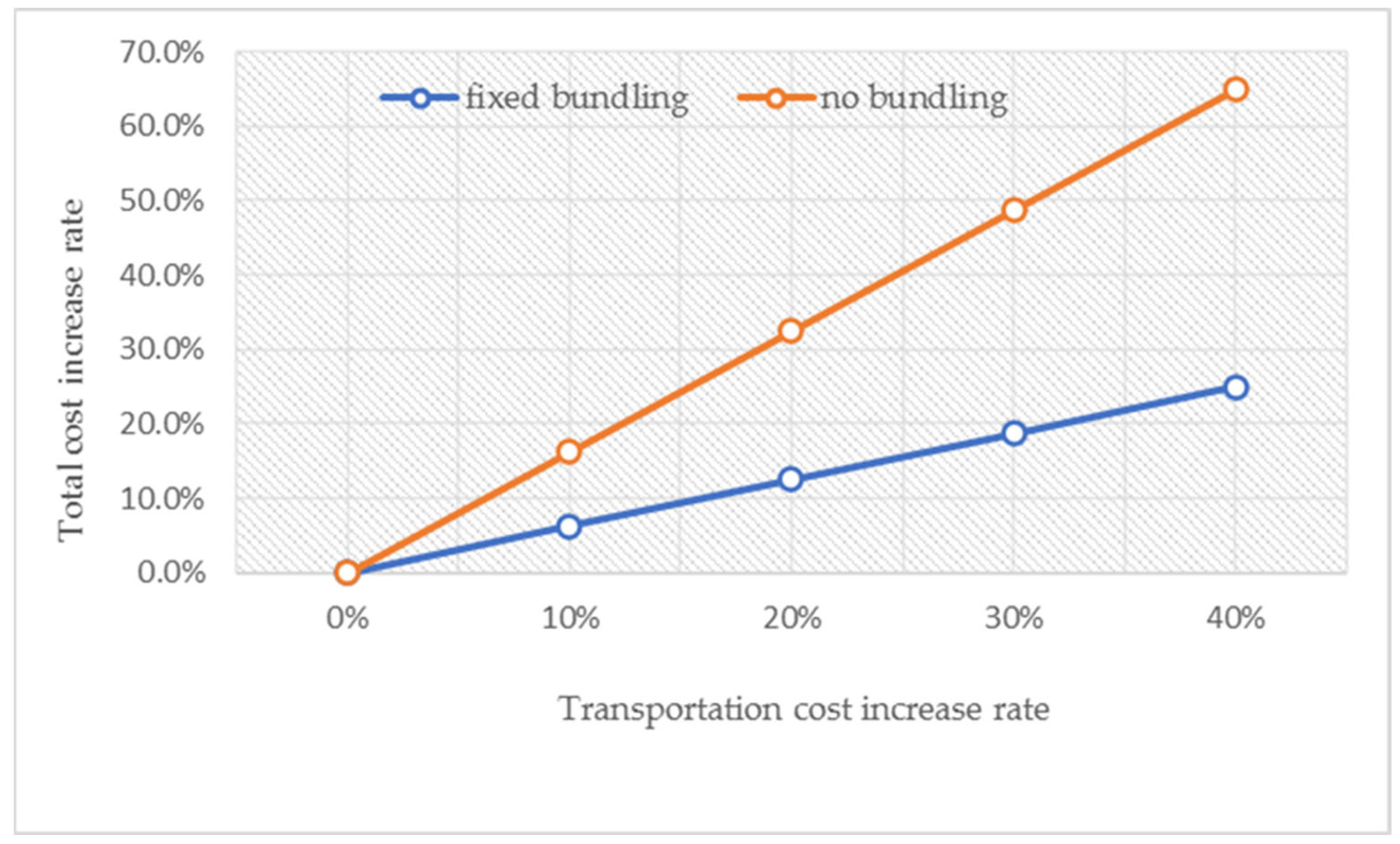
5.3. Sensitivity Analysis on Cost Parameters
6. Conclusions
Author Contributions
Funding
Conflicts of Interest
References
- Myung, Y.S.; Yu, Y.M. Freight transportation network model with bundling option. Transp. Res. Part E 2020, 133, 101827. [Google Scholar] [CrossRef]
- Fanti, M.P.; Mangini, A.M.; Roccotelli, M. Innovative Approaches for Electric Vehicles Relocation in Sharing Systems. IEEE Trans. Autom. Sci. Eng. 2022, 19, 21–36. [Google Scholar] [CrossRef]
- Zhang, S.; Zhao, X.; Li, X.; Yu, H. Heterogeneous fleet management for one-way electric carsharing system with optional orders, vehicle relocation and on-demand recharging. Comput. Oper. Res. 2022, 145, 105868. [Google Scholar] [CrossRef]
- Fanti, M.P.; Mangini, A.M.; Roccotelli, M. Hospital Drugs Distribution with Autonomous Robot Vehicles. In Proceedings of the IEEE 16th International Conference on Automation Science and Engineering (CASE), Hong Kong, China, 20–21 August 2020. [Google Scholar]
- Myung, Y.S.; Moon, I.K.; Lee, J.H.; Lee, K.S. Analyzing the effects of using both foldable and standard containers in ocean transportation. Int. J. Ind. Eng. 2021, 28, 92–105. [Google Scholar]
- Konings, R.; Thijs, R. Foldable containers: A new perspective on reducing container-repositioning costs. Eur. J. Oper. Res. 2001, 1, 333–352. [Google Scholar]
- Konings, R. Foldable containers to reduce the costs of empty transport? A cost–benefit analysis from a chain and multi-actor perspective. Marit. Econ. Logist. 2005, 7, 223–249. [Google Scholar] [CrossRef]
- Goh, S.H. The impact of foldable ocean containers on back haul shippers and carbon emissions. Transp. Res. Part D 2019, 67, 514–527. [Google Scholar] [CrossRef]
- Shintani, K.; Konings, R.; Imai, A. The impact of foldable containers on container fleet management costs in hinterland transport. Transp. Res. Part E 2010, 46, 750–763. [Google Scholar] [CrossRef]
- Ahuja, R.K.; Magnanti, T.L.; Orlin, J.B. Network Flows; Prentice-Hall: Hoboken, NJ, USA, 1993. [Google Scholar]
- Fortune, S.; Hopcroft, J.; Wyllie, J. The directed subgraph homeomorphism problem. Theor. Comput. Sci. 1980, 10, 111–121. [Google Scholar] [CrossRef] [Green Version]
- Myung, Y.S. Efficient solution methods for the integer programming models of relocating empty containers in the hinterland transportation network. Transp. Res. Part E 2017, 108, 52–59. [Google Scholar] [CrossRef]


| No. of Nodes | Network Density | z(LP) (=z(LPV)) | Fixed Bundling (4 Flows) | Variable Bundling (2, 3, 4 Flows) | Computation Time (Seconds) | ||||||||
|---|---|---|---|---|---|---|---|---|---|---|---|---|---|
| z(H) | z(P) | z(HV) | z(PV) | Fixed Bundling | Variable Bundling | ||||||||
| H | P | HV | PV | ||||||||||
| 30 | 0.2 | 38,549.5 | 42,539.0 | 41,601.9 | 1.02 | 40,706.0 | 39,962.1 | 1.02 | 0.040 | 0.016 | 0.140 | 0.015 | 0.922 |
| 47,824.9 | 54,648.8 | 50,349.3 | 1.09 | 50,560.7 | 49,463.0 | 1.02 | 0.047 | 0.016 | 0.031 | 0.016 | 0.141 | ||
| 43,534.2 | 47,719.7 | 46,425.8 | 1.03 | 45,825.9 | 45,021.2 | 1.02 | 0.041 | 0.015 | 0.031 | 0.016 | 0.219 | ||
| 43,587.3 | 47,666.3 | 46,574.2 | 1.02 | 45,633.4 | 45,063.5 | 1.01 | 0.041 | 0.000 | 0.156 | 0.016 | 0.203 | ||
| 52,826.2 | 56,334.6 | 55,617.7 | 1.01 | 54,618.6 | 54,229.6 | 1.01 | 0.052 | 0.000 | 0.172 | 0.016 | 0.203 | ||
| 0.35 | 38,696.8 | 43,149.5 | 41,521.0 | 1.04 | 40,792.1 | 40,114.5 | 1.02 | 0.057 | 0.016 | 0.062 | 0.015 | 0.313 | |
| 38,823.8 | 44,551.0 | 41,707.9 | 1.07 | 40,722.0 | 39,944.5 | 1.02 | 0.061 | 0.015 | 0.157 | 0.015 | 0.281 | ||
| 35,866.6 | 40,062.2 | 38,115.4 | 1.05 | 37,577.8 | 37,010.0 | 1.02 | 0.059 | 0.000 | 0.016 | 0.015 | 0.094 | ||
| 50,049.2 | 53,963.7 | 52,638.6 | 1.03 | 51,701.1 | 51,221.5 | 1.01 | 0.045 | 0.015 | 0.062 | 0.015 | 0.110 | ||
| 55,603.9 | 60,421.6 | 58,252.0 | 1.04 | 57,348.5 | 56,787.5 | 1.01 | 0.081 | 0.000 | 0.047 | 0.016 | 0.532 | ||
| 0.5 | 43,031.2 | 47,271.1 | 45,090.2 | 1.05 | 44,671.6 | 44,071.4 | 1.01 | 0.070 | 0.016 | 0.187 | 0.000 | 0.125 | |
| 49,047.1 | 53,341.2 | 51,461.8 | 1.04 | 50,919.7 | 50,119.6 | 1.02 | 0.069 | 0.016 | 0.031 | 0.016 | 0.922 | ||
| 38,438.8 | 41,805.1 | 40,575.1 | 1.03 | 40,108.8 | 39,449.0 | 1.02 | 0.077 | 0.015 | 0.031 | 0.015 | 0.204 | ||
| 35,062.6 | 39,249.0 | 37,650.1 | 1.04 | 36,598.9 | 36,079.9 | 1.01 | 0.072 | 0.015 | 0.047 | 0.000 | 0.563 | ||
| 40,583.1 | 44,910.4 | 42,888.7 | 1.05 | 42,182.9 | 41,614.5 | 1.01 | 0.066 | 0.000 | 0.078 | 0.015 | 0.047 | ||
| 50 | 0.2 | 65,654.5 | 72,172.3 | 70,076.1 | 1.03 | 68,339.1 | 67,642.0 | 1.01 | 0.173 | 0.015 | 0.078 | 0.016 | 2.297 |
| 83,393.9 | 90,722.6 | 87,804.1 | 1.03 | 86,808.7 | 85,706.0 | 1.01 | 0.152 | 0.031 | 0.313 | 0.032 | 3.422 | ||
| 70,942.3 | 78,581.1 | 75,902.0 | 1.04 | 74,380.0 | 73,303.8 | 1.01 | 0.225 | 0.031 | 0.906 | 0.015 | 1.656 | ||
| 73,521.7 | 85,272.2 | 78,470.3 | 1.09 | 77,313.7 | 75,510.1 | 1.02 | 0.163 | 0.016 | 0.172 | 0.031 | 9.609 | ||
| 62,195.5 | 69,916.0 | 66,989.6 | 1.04 | 64,856.0 | 64,102.1 | 1.01 | 0.193 | 0.032 | 0.484 | 0.015 | 1.750 | ||
| 0.35 | 72,482.7 | 78,083.1 | 76,479.0 | 1.02 | 75,419.6 | 74,381.0 | 1.01 | 0.280 | 0.016 | 0.062 | 0.032 | 1.922 | |
| 76,501.8 | 82,677.1 | 79,786.8 | 1.04 | 79,333.6 | 78,298.4 | 1.01 | 0.248 | 0.016 | 0.219 | 0.015 | 4.750 | ||
| 59,078.6 | 64,856.8 | 62,615.7 | 1.04 | 61,520.2 | 60,565.3 | 1.02 | 0.277 | 0.015 | 0.594 | 0.016 | 0.094 | ||
| 66,049.0 | 71,739.3 | 69,624.9 | 1.03 | 68,850.5 | 67,677.9 | 1.02 | 0.259 | 0.000 | 0.109 | 0.016 | 0.312 | ||
| 76,655.7 | 84,447.3 | 80,168.9 | 1.05 | 79,455.8 | 78,386.6 | 1.01 | 0.245 | 0.015 | 0.531 | 0.016 | 0.344 | ||
| 0.5 | 66,734.2 | 73,623.3 | 70,021.4 | 1.05 | 69,737.5 | 68,367.6 | 1.02 | 0.356 | 0.015 | 0.047 | 0.016 | 2.641 | |
| 61,783.8 | 68,200.9 | 64,947.6 | 1.05 | 64,280.9 | 63,236.6 | 1.02 | 0.316 | 0.016 | 0.094 | 0.016 | 3.657 | ||
| 65,038.7 | 71,631.1 | 68,602.4 | 1.04 | 68,171.1 | 66,582.8 | 1.02 | 0.320 | 0.016 | 0.094 | 0.016 | 0.359 | ||
| 60,479.2 | 65,102.8 | 63,433.6 | 1.03 | 62,707.7 | 62,178.3 | 1.01 | 0.311 | 0.015 | 0.094 | 0.016 | 3.454 | ||
| 61,454.2 | 67,887.9 | 65,143.4 | 1.04 | 64,547.9 | 63,050.1 | 1.02 | 0.329 | 0.000 | 0.235 | 0.015 | 0.218 | ||
| 100 | 0.2 | 146,960.1 | 164,015.2 | 156,708.2 | 1.05 | 153,541.8 | 150,929.9 | 1.02 | 1.210 | 0.047 | 1.734 | 0.078 | 12.796 |
| 139,430.4 | 152,570.0 | 147,260.6 | 1.04 | 144,612.9 | 142,853.9 | 1.01 | 1.490 | 0.047 | 0.656 | 0.047 | 9.875 | ||
| 145,488.5 | 159,903.8 | 152,864.1 | 1.05 | 152,069.9 | 148,858.2 | 1.02 | 1.621 | 0.047 | 0.672 | 0.047 | 55.578 | ||
| 123,636.1 | 136,175.0 | 130,979.2 | 1.04 | 129,559.9 | 127,267.9 | 1.02 | 1.366 | 0.047 | 0.391 | 0.047 | 9.453 | ||
| 119,307.7 | 134,006.3 | 127,662.3 | 1.05 | 124,966.4 | 122,427.7 | 1.02 | 1.445 | 0.047 | 0.125 | 0.047 | 7.688 | ||
| 0.35 | 134,472.5 | 148,102.7 | 142,055.3 | 1.04 | 139,734.9 | 137,366.7 | 1.02 | 1.883 | 0.062 | 1.703 | 0.047 | 9.922 | |
| 122,559.9 | 133,704.0 | 129,525.1 | 1.03 | 127,554.3 | 125,828.0 | 1.01 | 2.244 | 0.047 | 0.422 | 0.047 | 19.125 | ||
| 118,575.4 | 132,031.8 | 124,750.1 | 1.06 | 123,753.5 | 121,430.6 | 1.02 | 2.160 | 0.047 | 0.688 | 0.047 | 21.907 | ||
| 130,914.7 | 143,417.9 | 137,824.0 | 1.04 | 136,181.9 | 134,124.9 | 1.02 | 1.944 | 0.047 | 0.640 | 0.047 | 21.046 | ||
| 125,046.0 | 137,495.1 | 131,992.0 | 1.04 | 130,436.7 | 127,882.4 | 1.02 | 2.126 | 0.031 | 4.657 | 0.046 | 5.297 | ||
| 0.5 | 146,731.0 | 158,146.4 | 152,674.0 | 1.04 | 151,804.5 | 149,469.8 | 1.02 | 2.330 | 0.047 | 2.047 | 0.062 | 16.265 | |
| 122,944.1 | 138,228.5 | 129,992.6 | 1.06 | 129,351.5 | 126,177.7 | 1.03 | 2.524 | 0.047 | 2.329 | 0.062 | 12.078 | ||
| 136,517.8 | 148,486.0 | 143,227.9 | 1.04 | 141,608.0 | 139,609.2 | 1.01 | 2.548 | 0.047 | 2.093 | 0.063 | 13.469 | ||
| 118,029.5 | 129,556.4 | 125,118.5 | 1.04 | 123,180.7 | 120,869.9 | 1.02 | 2.820 | 0.047 | 0.313 | 0.062 | 9.078 | ||
| 140,466.3 | 154,376.5 | 147,246.7 | 1.05 | 146,390.1 | 143,179.2 | 1.02 | 3.112 | 0.047 | 0.375 | 0.047 | >200.0 | ||
| No. of Nodes | Network Density | z(LP) (=z(LPV)) | Fixed Bundling (4 Flows) | Variable Bundling (2, 3, 4 Flows) | Computation Time (Seconds) | ||||||||
|---|---|---|---|---|---|---|---|---|---|---|---|---|---|
| z(H) | z(P) | z(HV) | z(PV) | Fixed Bundling | Variable Bundling | ||||||||
| H | P | HV | PV | ||||||||||
| 150 | 0.2 | 186,021.5 | 204,181.1 | 197,090.8 | 1.04 | 194,335.7 | 190,779.7 | 1.02 | 4.712 | 0.094 | 4.969 | 0.125 | 118.766 |
| 188,070.4 | 208,907.5 | 198,984.1 | 1.05 | 195,516.2 | 192,528.2 | 1.02 | 4.964 | 0.078 | 0.641 | 0.109 | 141.703 | ||
| 186,269.4 | 205,067.3 | 196,351.6 | 1.04 | 194,197.6 | 190,906.1 * | 1.02 | 5.228 | 0.078 | 7.094 | 0.110 | >200.0 | ||
| 206,545.3 | 223,887.6 | 215,596.7 | 1.04 | 214,162.7 | 210,652.5 | 1.02 | 4.416 | 0.094 | 7.390 | 0.109 | 21.204 | ||
| 212,834.5 | 230,929.9 | 223,722.4 | 1.03 | 220,362.9 | 217,391.8 | 1.01 | 4.285 | 0.078 | 1.281 | 0.110 | 75.844 | ||
| 0.35 | 189,241.8 | 211,102.6 | 201,005.8 | 1.05 | 197,121.9 | 193,543.3 * | 1.02 | 7.584 | 0.094 | 3.672 | 0.109 | >200.0 | |
| 178,520.3 | 196,661.3 | 187,720.7 | 1.05 | 185,855.2 | 183,075.6 | 1.02 | 6.879 | 0.094 | 4.844 | 0.125 | 56.578 | ||
| 184,497.0 | 203,573.0 | 193,797.2 | 1.05 | 192,182.3 | 188,732.3 | 1.02 | 7.234 | 0.094 | 0.875 | 0.125 | 45.563 | ||
| 207,419.5 | 227,116.2 | 216,735.3 | 1.05 | 215,632.5 | 211,834.1 * | 1.02 | 8.221 | 0.094 | 5.657 | 0.125 | >200.0 | ||
| 204,764.9 | 222,671.6 | 215,092.5 | 1.04 | 212,387.1 | 209,213.9 | 1.02 | 6.344 | 0.093 | 7.313 | 0.109 | 90.047 | ||
| 0.5 | 197,161.2 | 215,351.0 | 206,805.7 | 1.04 | 204,896.9 | 201,486.8 | 1.02 | 8.728 | 0.093 | 1.641 | 0.125 | 116.718 | |
| 210,401.5 | 233,013.5 | 221,104.5 | 1.05 | 219,275.0 | 215,081.3 * | 1.02 | 10.717 | 0.094 | 5.343 | 0.125 | >200.0 | ||
| 194,887.8 | 211,789.2 | 203,918.5 | 1.04 | 202,195.5 | 199,057.0 | 1.02 | 9.034 | 0.094 | 5.078 | 0.125 | 33.562 | ||
| 186,103.7 | 203,894.8 | 195,185.6 | 1.04 | 193,597.0 | 190,209.0 | 1.02 | 9.803 | 0.094 | 0.640 | 0.125 | 145.203 | ||
| 187,789.4 | 204,577.5 | 196,484.6 | 1.04 | 195,152.1 | 191,703.6 | 1.02 | 9.638 | 0.109 | 4.984 | 0.125 | 21.406 | ||
| 200 | 0.2 | 265,694.2 | 293,003.9 | 278,242.9 | 1.05 | 276,052.6 | 271,971.4 | 1.02 | 12.410 | 0.140 | 7.922 | 0.188 | 123.297 |
| 266,388.3 | 291,343.4 | 279,358.2 | 1.04 | 276,870.0 | 273,194.1* | 1.01 | 11.664 | 0.140 | 18.468 | 0.187 | >200.0 | ||
| 248,625.7 | 273,959.3 | 261,703.3 | 1.05 | 258,930.9 | 254,429.8 | 1.02 | 10.829 | 0.125 | 0.641 | 0.188 | 89.141 | ||
| 268,625.2 | 294,868.9 | 282,156.2 | 1.05 | 278,275.1 | 275,047.2 | 1.01 | 10.607 | 0.141 | 5.563 | 0.188 | 196.234 | ||
| 255,943.2 | 278,715.7 | 269,754.2 | 1.03 | 266,170.3 | 261,899.1 | 1.02 | 12.082 | 0.125 | 10.735 | 0.188 | 174.531 | ||
| 0.35 | 241,651.2 | 267,602.9 | 255,854.2 | 1.05 | 251,881.6 | 248,194.0 * | 1.01 | 17.203 | 0.157 | 11.203 | 0.203 | >200.0 | |
| 274,468.4 | 301,392.9 | 288,321.0 | 1.05 | 286,237.9 | 280,967.8 | 1.02 | 14.427 | 0.156 | 14.312 | 0.203 | 162.766 | ||
| 227,371.3 | 250,405.0 | 239,909.0 | 1.04 | 237,649.8 | 233,377.8 * | 1.02 | 17.032 | 0.157 | 1.516 | 0.203 | >200.0 | ||
| 233,471.7 | 258,764.2 | 247,295.5 | 1.05 | 243,761.9 | 239,771.0 * | 1.02 | 17.494 | 0.156 | 10.640 | 0.219 | >200.0 | ||
| 241,197.5 | 264,796.7 | 254,017.2 | 1.04 | 251,706.0 | 247,170.7 | 1.02 | 16.763 | 0.156 | 12.562 | 0.203 | 128.531 | ||
| 0.5 | 239,972.6 | 266,232.1 | 253,593.7 | 1.05 | 251,442.3 | 246,094.4 | 1.02 | 21.883 | 0.172 | 9.063 | 0.203 | 162.250 | |
| 249,999.4 | 274,186.4 | 262,683.9 | 1.04 | 260,445.8 | 255,702.6 * | 1.02 | 23.178 | 0.156 | 25.765 | 0.219 | >200.0 | ||
| 278,675.3 | 304,443.6 | 292,660.9 | 1.04 | 289,547.9 | 284,612.7 | 1.02 | 24.684 | 0.157 | 10.828 | 0.219 | 127.688 | ||
| 227,237.9 | 249,030.6 | 239,973.2 | 1.04 | 236,377.7 | 232,500.0 * | 1.02 | 21.410 | 0.172 | 5.938 | 0.250 | >200.0 | ||
| 254,442.1 | 277,356.8 | 267,816.0 | 1.04 | 265,929.7 | 260,642.1 * | 1.02 | 20.238 | 0.156 | 17.922 | 0.218 | >200.0 | ||
| 300 | 0.2 | 371,125.3 | 405,564.8 | 390,230.0 | 1.04 | 386,303.6 | 379,983.8 * | 1.02 | 37.315 | 0.344 | 6.421 | 0.438 | >200.0 |
| 342,360.5 | 377,712.9 | 361,157.6 | 1.05 | 358,140.1 | 351,449.3 | 1.02 | 37.939 | 0.344 | 3.204 | 0.438 | 125.703 | ||
| 344,723.9 | 381,496.4 | 363,880.3 | 1.05 | 360,203.9 | 354,247.7 | 1.02 | 39.551 | 0.344 | 6.937 | 0.453 | 157.984 | ||
| 389,669.2 | 429,196.4 | 410,803.9 | 1.04 | 406,603.1 | 399,348.4 | 1.02 | 41.357 | 0.329 | 14.391 | 0.438 | 195.078 | ||
| 377,427.3 | 412,750.1 | 397,185.5 | 1.04 | 392,556.2 | 386,124.4 | 1.02 | 36.834 | 0.360 | 14.328 | 0.453 | 143.375 | ||
| 0.35 | 343,722.0 | 376,945.2 | 361,726.6 | 1.04 | 359,051.1 | 352,210.5 | 1.02 | 58.442 | 0.375 | 4.875 | 0.485 | 83.031 | |
| 349,822.5 | 381,646.7 | 367,922.9 | 1.04 | 364,278.9 | 358,513.1 | 1.02 | 56.283 | 0.406 | 16.985 | 0.484 | 196.140 | ||
| 351,332.3 | 388,453.7 | 370,903.1 | 1.05 | 365,432.9 | 359,823.9 | 1.02 | 57.514 | 0.375 | 18.703 | 0.469 | 98.829 | ||
| 382,843.8 | 415,349.7 | 401,904.0 | 1.03 | 397,551.3 | 391,594.8 | 1.02 | 53.727 | 0.406 | 30.703 | 0.500 | 100.547 | ||
| 355,320.6 | 386,656.1 | 373,225.0 | 1.04 | 369,290.6 | 364,022.3 | 1.01 | 59.228 | 0.375 | 2.735 | 0.468 | 155.594 | ||
| 0.5 | 388,961.1 | 424,683.6 | 407,933.9 | 1.04 | 403,916.8 | 396,804.5 * | 1.02 | 69.960 | 0.375 | 21.047 | 0.500 | >200.0 | |
| 379,047.1 | 418,412.8 | 398,560.6 | 1.05 | 394,950.3 | 387,871.5 | 1.02 | 83.034 | 0.375 | 7.312 | 0.500 | 145.656 | ||
| 391,175.6 | 424,843.9 | 409,062.4 | 1.04 | 406,694.3 | 399,240.7 | 1.02 | 81.193 | 0.391 | 4.547 | 0.484 | 100.062 | ||
| 353,861.8 | 388,483.2 | 372,150.8 | 1.04 | 369,322.6 | 361,983.0 | 1.02 | 77.186 | 0.375 | 12.656 | 0.500 | 196.875 | ||
| 361,084.0 | 394,074.2 | 377,812.9 | 1.04 | 376,775.0 | 369,063.3 | 1.02 | 77.923 | 0.422 | 1.938 | 0.469 | 96.250 | ||
| No. of Nodes | Network Density | No Bundling (a) | FTNPB (without B\UB Restriction) | FTNPB-R (with B\UB Restriction) | ||||||
|---|---|---|---|---|---|---|---|---|---|---|
| Fixed Bundling (b) | (b/a) | Variable Bundling (c) | (c/a) | Fixed Bundling (d) | (d/a) | Variable Bundling (e) | (e/a) | |||
| 50 | 0.2 | 150,634.1 | 69,505.2 | 0.46 | 67,626.6 | 0.45 | 70,076.1 | 0.47 | 67,642.0 | 0.45 |
| 183,959.8 | 86,960.0 | 0.47 | 85,523.1 | 0.46 | 87,804.1 | 0.48 | 85,706.0 | 0.47 | ||
| 164,349.2 | 74,860.5 | 0.46 | 73,152.1 | 0.45 | 75,902.0 | 0.46 | 73,304.2 | 0.45 | ||
| 187,986.8 | 77,555.2 | 0.41 | 75,366.9 | 0.40 | 78,470.3 | 0.42 | 75,510.1 | 0.40 | ||
| 130,453.8 | 65,804.1 | 0.50 | 64,102.1 | 0.49 | 66,989.6 | 0.51 | 64,102.1 | 0.49 | ||
| 0.35 | 136,158.9 | 76,056.8 | 0.56 | 74,381.0 | 0.55 | 76,479.0 | 0.56 | 74,381.0 | 0.55 | |
| 147,811.2 | 79,342.3 | 0.54 | 78,298.4 | 0.53 | 79,786.8 | 0.54 | 78,298.4 | 0.53 | ||
| 129,450.3 | 62,021.5 | 0.48 | 60,565.3 | 0.47 | 62,615.7 | 0.48 | 60,565.3 | 0.47 | ||
| 138,983.9 | 69,001.4 | 0.50 | 67,677.9 | 0.49 | 69,624.9 | 0.50 | 67,677.9 | 0.49 | ||
| 151,634.9 | 79,964.8 | 0.53 | 78,386.6 | 0.52 | 80,168.9 | 0.53 | 78,386.7 | 0.52 | ||
| 0.5 | 139,196.7 | 69,601.6 | 0.50 | 68,367.6 | 0.49 | 70,021.4 | 0.50 | 68,369.3 | 0.49 | |
| 128,955.2 | 64,577.6 | 0.50 | 63,236.6 | 0.49 | 64,947.6 | 0.50 | 63,236.6 | 0.49 | ||
| 131,510.8 | 68,020.0 | 0.52 | 66,582.8 | 0.51 | 68,602.4 | 0.52 | 66,582.8 | 0.51 | ||
| 120,749.0 | 63,244.5 | 0.52 | 62,175.5 | 0.51 | 63,433.6 | 0.53 | 62,178.3 | 0.51 | ||
| 130,884.8 | 64,568.0 | 0.49 | 63,050.1 | 0.48 | 65,143.4 | 0.50 | 63,050.1 | 0.48 | ||
| No. of Nodes | Network Density | Original Data (a) | 10% Increase | 20% Increase | 30% Increase | 40% Increase | ||||
|---|---|---|---|---|---|---|---|---|---|---|
| (b) | (c) | (b) | (c) | (b) | (c) | (b) | (c) | |||
| (No Bundling Case) | ||||||||||
| 50 | 0.2 | 150,634.10 | 165,697.50 | 10.00% | 180,760.90 | 20.00% | 195,824.30 | 30.00% | 210,887.70 | 40.00% |
| 183,959.80 | 202,355.70 | 10.00% | 220,751.70 | 20.00% | 239,147.70 | 30.00% | 257,543.70 | 40.00% | ||
| 164,349.20 | 180,784.10 | 10.00% | 197,219.00 | 20.00% | 213,654.00 | 30.00% | 230,088.90 | 40.00% | ||
| 187,986.80 | 206,785.50 | 10.00% | 225,584.20 | 20.00% | 244,382.90 | 30.00% | 263,181.60 | 40.00% | ||
| 130,453.80 | 143,499.20 | 10.00% | 156,544.60 | 20.00% | 169,590.00 | 30.00% | 182,635.40 | 40.00% | ||
| 0.35 | 136,158.90 | 149,774.80 | 10.00% | 163,390.70 | 20.00% | 177,006.60 | 30.00% | 190,622.40 | 40.00% | |
| 147,811.20 | 162,592.30 | 10.00% | 177,373.40 | 20.00% | 192,154.60 | 30.00% | 206,935.70 | 40.00% | ||
| 129,450.30 | 142,395.30 | 10.00% | 155,340.30 | 20.00% | 168,285.40 | 30.00% | 181,230.40 | 40.00% | ||
| 138,983.90 | 152,882.30 | 10.00% | 166,780.70 | 20.00% | 180,679.10 | 30.00% | 194,577.50 | 40.00% | ||
| 151,634.90 | 166,798.40 | 10.00% | 181,961.90 | 20.00% | 197,125.30 | 30.00% | 212,288.80 | 40.00% | ||
| 0.5 | 139,196.70 | 153,116.40 | 10.00% | 167,036.10 | 20.00% | 180,955.70 | 30.00% | 194,875.40 | 40.00% | |
| 128,955.20 | 141,850.70 | 10.00% | 154,746.20 | 20.00% | 167,641.70 | 30.00% | 180,537.20 | 40.00% | ||
| 131,510.80 | 144,661.90 | 10.00% | 157,813.00 | 20.00% | 170,964.00 | 30.00% | 184,115.10 | 40.00% | ||
| 120,749.00 | 132,823.90 | 10.00% | 144,898.80 | 20.00% | 156,973.70 | 30.00% | 169,048.60 | 40.00% | ||
| 130,884.80 | 143,973.30 | 10.00% | 157,061.80 | 20.00% | 170,150.30 | 30.00% | 183,238.80 | 40.00% | ||
| (Fixed bundling case) | ||||||||||
| 50 | 0.2 | 70,076.10 | 74,442.50 | 6.20% | 78,808.90 | 12.50% | 83,175.30 | 18.70% | 87,541.80 | 24.90% |
| 87,804.10 | 93,030.90 | 6.00% | 98,257.70 | 11.90% | 103,484.50 | 17.90% | 108,711.30 | 23.80% | ||
| 75,902.00 | 80,677.40 | 6.30% | 85,448.10 | 12.60% | 90,218.80 | 18.90% | 94,989.40 | 25.10% | ||
| 78,470.30 | 83,854.50 | 6.90% | 89,238.70 | 13.70% | 94,623.00 | 20.60% | 100,007.20 | 27.40% | ||
| 66,989.60 | 70,892.10 | 5.80% | 74,794.70 | 11.70% | 78,697.20 | 17.50% | 82,599.80 | 23.30% | ||
| 0.35 | 76,479.00 | 80,515.80 | 5.30% | 84,552.50 | 10.60% | 88,589.20 | 15.80% | 92,625.90 | 21.10% | |
| 79,786.80 | 84,002.20 | 5.30% | 88,217.70 | 10.60% | 92,433.20 | 15.90% | 96,648.70 | 21.10% | ||
| 62,615.70 | 66,350.50 | 6.00% | 70,085.20 | 11.90% | 73,820.00 | 17.90% | 77,554.80 | 23.90% | ||
| 69,624.90 | 73,651.40 | 5.80% | 77,677.90 | 11.60% | 81,704.30 | 17.30% | 85,730.80 | 23.10% | ||
| 80,168.90 | 84,509.00 | 5.40% | 88,849.00 | 10.80% | 93,189.10 | 16.20% | 97,529.20 | 21.70% | ||
| 0.5 | 70,021.40 | 74,003.20 | 5.70% | 77,984.90 | 11.40% | 81,966.70 | 17.10% | 85,948.40 | 22.70% | |
| 64,947.60 | 68,609.10 | 5.60% | 72,270.70 | 11.30% | 75,932.30 | 16.90% | 79,593.80 | 22.60% | ||
| 68,602.40 | 72,415.00 | 5.60% | 76,227.70 | 11.10% | 80,040.30 | 16.70% | 83,852.90 | 22.20% | ||
| 63,433.60 | 66,910.90 | 5.50% | 70,388.30 | 11.00% | 73,865.60 | 16.40% | 77,343.00 | 21.90% | ||
| 65,143.40 | 68,929.70 | 5.80% | 72,716.00 | 11.60% | 76,502.40 | 17.40% | 80,288.70 | 23.20% | ||
| No. of Nodes | Network Density | Original Data (a) | 10% Decrease | 20% Decrease | 30% Decrease | 40% Decrease | ||||
|---|---|---|---|---|---|---|---|---|---|---|
| (b) | (c) | (b) | (c) | (b) | (c) | (b) | (c) | |||
| 50 | 0.2 | 70,076.1 | 64,080.1 | 8.6% | 59,836.1 | 14.6% | 55,876.1 | 20.3% | 52,248.1 | 25.4% |
| 87,804.1 | 84,264.1 | 4.0% | 80,736.1 | 8.0% | 76,732.1 | 12.6% | 73,197.0 | 16.6% | ||
| 75,902.0 | 73,074.0 | 3.7% | 70,074.7 | 7.7% | 67,110.7 | 11.6% | 64,464.7 | 15.1% | ||
| 78,470.3 | 75,994.3 | 3.2% | 73,246.3 | 6.7% | 70,838.3 | 9.7% | 68,390.3 | 12.8% | ||
| 66,989.6 | 64,173.6 | 4.2% | 61,229.6 | 8.6% | 58,369.6 | 12.9% | 55,509.6 | 17.1% | ||
| 0.35 | 76,479.0 | 72,691.0 | 5.0% | 69,055.0 | 9.7% | 65,391.0 | 14.5% | 61,667.0 | 19.4% | |
| 79,786.8 | 75,930.8 | 4.8% | 72,242.8 | 9.5% | 68,294.2 | 14.4% | 64,274.2 | 19.4% | ||
| 62,615.7 | 60,115.7 | 4.0% | 57,483.7 | 8.2% | 54,847.7 | 12.4% | 52,191.7 | 16.6% | ||
| 69,624.9 | 66,588.9 | 4.4% | 63,692.9 | 8.5% | 60,516.9 | 13.1% | 57,592.9 | 17.3% | ||
| 80,168.9 | 76,416.9 | 4.7% | 72,520.9 | 9.5% | 68,912.9 | 14.0% | 65,040.9 | 18.9% | ||
| 0.5 | 70,021.4 | 66,949.4 | 4.4% | 63,785.4 | 8.9% | 60,697.4 | 13.3% | 57,521.4 | 17.9% | |
| 64,947.6 | 61,987.6 | 4.6% | 59,095.6 | 9.0% | 56,227.6 | 13.4% | 53,247.6 | 18.0% | ||
| 68,602.4 | 65,382.4 | 4.7% | 62,258.4 | 9.2% | 59,234.4 | 13.7% | 56,090.4 | 18.2% | ||
| 63,433.6 | 60,333.6 | 4.9% | 57,501.6 | 9.4% | 54,461.6 | 14.1% | 51,621.6 | 18.6% | ||
| 65,143.4 | 62,379.4 | 4.2% | 59,567.4 | 8.6% | 56,739.4 | 12.9% | 53,951.4 | 17.2% | ||
Publisher’s Note: MDPI stays neutral with regard to jurisdictional claims in published maps and institutional affiliations. |
© 2022 by the authors. Licensee MDPI, Basel, Switzerland. This article is an open access article distributed under the terms and conditions of the Creative Commons Attribution (CC BY) license (https://creativecommons.org/licenses/by/4.0/).
Share and Cite
Myung, Y.-S.; Yu, Y.-M. A Freight Transportation Network Model with a New Bundling Option. Sustainability 2022, 14, 7556. https://doi.org/10.3390/su14137556
Myung Y-S, Yu Y-M. A Freight Transportation Network Model with a New Bundling Option. Sustainability. 2022; 14(13):7556. https://doi.org/10.3390/su14137556
Chicago/Turabian StyleMyung, Young-Soo, and Yung-Mok Yu. 2022. "A Freight Transportation Network Model with a New Bundling Option" Sustainability 14, no. 13: 7556. https://doi.org/10.3390/su14137556
APA StyleMyung, Y.-S., & Yu, Y.-M. (2022). A Freight Transportation Network Model with a New Bundling Option. Sustainability, 14(13), 7556. https://doi.org/10.3390/su14137556