Prediction of Future Lake Water Availability Using SWAT and Support Vector Regression (SVR)

Abstract

Lakes are major surface water resource in semi-arid regions, providing water for agriculture and domestic use. Prediction of future water availability in lakes of semi-arid regions is important as they are highly sensitive to climate variability. This study is to examine the water level fluctuations in Pakhal Lake, Telangana, India using a combination of a process-based hydrological model and machine learning technique under climate change scenarios. Pakhal is an artificial lake built to meet the irrigation requirements of the region. Predictions of lake level can help with effective planning and management of water resources. In this study, an integrated approach is adopted to predict future water level fluctuations in Pakhal Lake in response to potential climate change. This study makes use of the NASA Earth Exchange Global Daily Downscaled Projections (NEX-GDDP) dataset which contains 21 Global Climate Models (GCMs) at a resolution of 0.25 × 0.25° is used for the study. The Reliability Ensemble Averaging (REA) method is applied to the 21 models to create an ensemble model. The hydrological model outputs from Soil and Water Assessment Tool (SWAT) are used to develop the machine-learning based Support Vector Regression (ν-SVR) model for predicting future water levels in Pakhal Lake. The scores of the three metrics, correlation coefficient (R²), RMSE and MEA are 0.79, 0.018 m, and 0.13 m, respectively for the training period. The values for the validation periods are 0.72, 0.6, and 0.25 m, indicating that the model captures the observed lake water level trends satisfactorily. The SWAT simulation results showed a decrease in surface runoff in the Representative Concentration Pathways (RCP) 4.5 scenario and an increase in the RCP 8.5 scenario. Further, the results from ν-SVR model for the future time period indicate a decrease in future lake levels during crop growth seasons. This study aids in planning of necessary water management options for Pakhal Lake under climate change scenarios. With limited observed datasets, this study can be easily extended to the other lake systems.

1. Introduction

Water is a natural resource that sustains life [1]. Water is used extensively by humans for a variety of purposes, including irrigation, residential, and industrial use. Climate change is a major determinant of water resource availability in a region [2,3]. It has a significant impact on the distribution of water resources both spatially and temporally. Significant changes in key hydro-climatological variables such as precipitation, temperature, evaporation, streamflow, and water level have been observed as a result of temperature excursions and climate change [4,5]. Climate change effects have become a major concern for water resource engineers and policymakers, particularly in arid and semi-arid regions [6,7,8,9,10]. Extreme precipitation events with significant spatiotemporal variability are common in arid and semi-arid regions [11,12]. Furthermore, rising temperatures in semi-arid regions are putting a strain on surface and groundwater availability [13,14,15]. Lakes are a critical source of water in semi-arid regions because they provide water for various purposes. The agricultural sector in these regions is highly dependent on the irrigation water supply from the lakes, as they play an important role in balancing the regional hydrological system [16,17]. The availability of lake water is directly attributed to the variation in climatic factors such as temperature, precipitation, and evaporation [18,19]. As a result, understanding the influence of climate change on lake water availability is critical for regional water resource planning and management.

Typically, the regional climate change impact analysis is carried out using hydrological modelling to obtain catchment water balance components using observational data and projecting them into the future using GCMs and RCMs [8,13,20,21,22,23,24,25]. SWAT-based hydrological modelling has enabled a large number of regional climate studies at the river basin and water-shed scale [23,26,27,28,29,30,31,32,33,34,35,36,37]. The SWAT model has the advantage of requiring little direct calibration to obtain good hydrologic predictions [36,37]. Recently, Saade et.al (2021) used the SWAT model for studying the impact of climate change on surface water availability in El Kalb River, Lebanon, which is a semi-arid basin [38]. Kwarteng et.al (2021) coupled the SWAT model with bathymetric data to simulate and estimate the water balance components of the Brimsu Reservoir [1]. SWAT model was used to understand the streamflow alterations in single and cascade lake systems located in the semi-arid region of India. These lake systems are ungauged and lack proper management options [8,13]. These studies provide insight into the present and future climate challenges on the lake water resource systems.

Apart from studying the impact of climate change on the lake water balance components, estimating lake level fluctuations under future climate scenarios is important for developing sustainable water management policies [39]. The natural water exchange between the lake and its catchment affects lake water level fluctuations, which reflect regional climatic variations [40]. Recently, machine learning-based Support Vector Machine (SVM) has been used effectively for predicting changes in water levels [41,42]. Khan and Coulibaly (2006) [43] investigated the utility of SVM in predicting lake water levels in Lake Erie over the long term. They observed that SVM outperformed multilayer perceptron (MLP). Cimen and Kisi (2009) [44] found that Support Vector Regression (SVR) outperformed Artificial Neural Networks (ANN) techniques in modeling the monthly lake levels. Hipni et al. (2013) found that the ν-SVR model outperformed the other SVM techniques in forecasting daily water levels in Klang reservoir, Malaysia, and concluded that the SVR model was the best regression type for lake water predictions [45]. Kisi et al. (2015) forecasted daily lake water levels in Lake Urmia using the SVM technique combined with the firefly algorithm [40]. Bucak et al. (2017) combined SWAT model outputs with the SVR model to forecast future water availability in Lake Beyşehir and concluded that climate change will cause the lake to dry up by the end of the century [39].

Previous studies primarily focused on assessing the effects of climate change on water balance components such as runoff, streamflow, and evapotranspiration in lake catchments. The majority of studies on the applicability of SVM techniques for lake level predictions were conducted using past lake levels, without taking into account the water balance components that influence water availability. Few studies have looked at how catchment hydrology and lake water level changes interact. The main objective of this study is to quantify the effects of climate change on water availability in Pakhal Lake, Telangana, India, and to evaluate the feasibility of the SVR approach for predicting lake water levels under current and future climate change scenarios. The Pakhal lake, located in a semi-arid region, is an important source of water for agriculture. This region’s poor and marginal farmers rely heavily on the lake for agricultural water. It is critical to investigate the impact of climate change on this lake system for future water resource planning and management in order to provide farmers with a sustainable livelihood. As a result, this study examines water availability and lake water fluctuations for current and future climate change scenarios for Phakal lake.

2. Materials and Methods

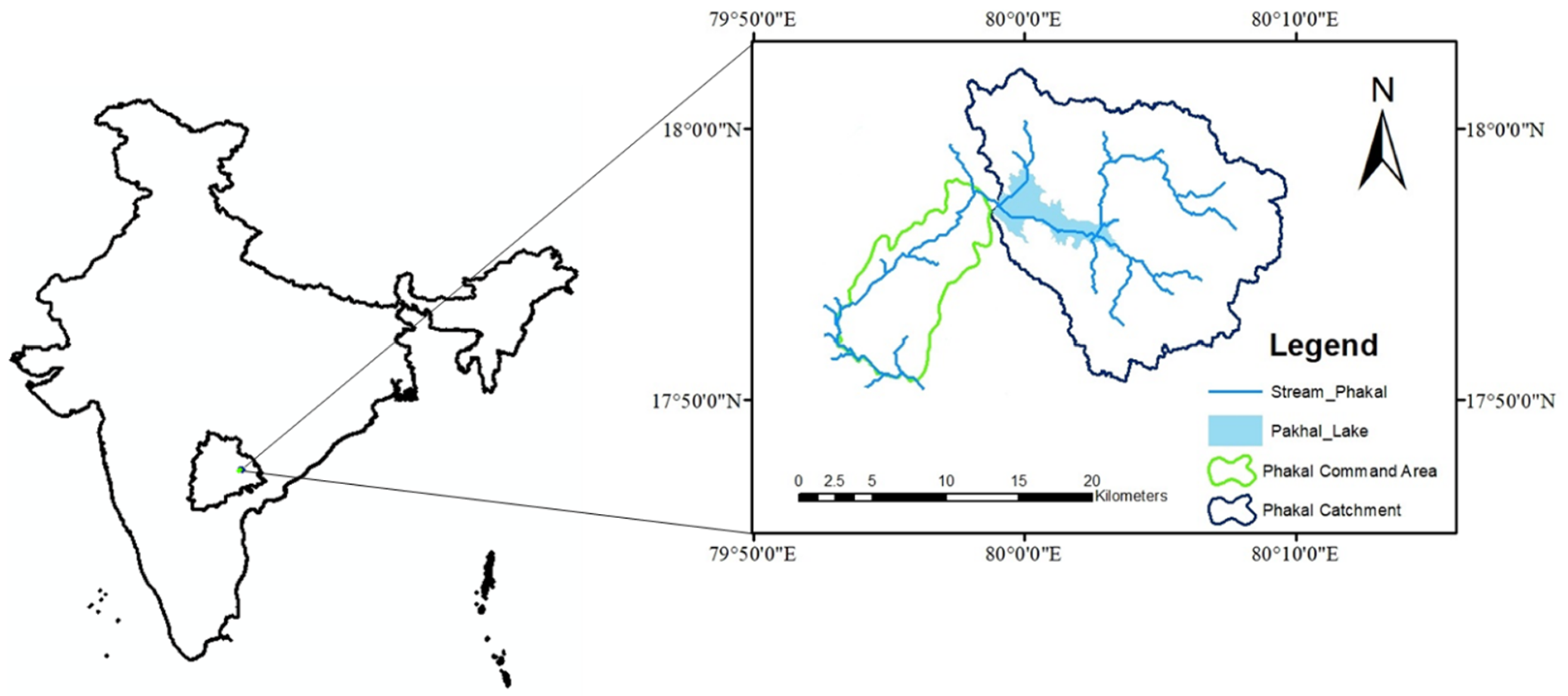
2.1. Study Area Description

The Pakhal lake is situated in Warangal district, Telangana, India, with its command area in Mahbubabad district. Figure 1 depicts the location map of Phakal lake, its catchment area, and command area. It is an artificial lake constructed by Kakatiya rulers on the Munneruvagu tributary of the Krishna River to provide irrigation water to the surrounding semiarid regions. The average rainfall in the study area is about 1000 mm. The minimum and maximum temperatures varies from 15 °C to 45 °C, respectively. The Pakhal lake is spread over an area of 30 km² and drawing water from a catchment area of 271.95 km², with a storage capacity of 95.86 Mm³. The lake is the main source of agricultural water for the surrounding villages. The Pakhal Lake was designed to irrigate 30,000 acres, but according to modern official figures, it only irrigates 18,193 acres. According to annual crop area statistics from Irrigation & CAD Department of Telangana, India [46], over 70% of this command area is cultivated in the Kharif season and just 30% in the rabi season (Figure 2). This is due to a shortage of lake water availability during the rabi season. As a result, the Telangana State Irrigation department planned to stabilise Pakhal Lake’s command area by linking it with Ramappa Lake. The linking project started its operation in April 2021, under which Pakhal Lake receives water from the Godavari River during the rabi season. Before planning the lake water augmentation by different methods, it is important to study current and future lake water availability under various climate change scenarios.

2.2. Methodology

The lack of observational data in the study area makes it difficult to set up a hydrological model for the catchment (ungauged) and predict future water availability in the lake, which is a major challenge for these studies. The hydrological modeling for the Pakhal catchment area was addressed using regionalization approach in Jayanthi and Keesara [13]. Because the Pakhal watershed lacks a gauge station, the SWAT model was put up for the Konduru watershed, which is located downstream of the present study area. The proximity method is used to transfer parameters from the source watershed to the Pakhal watershed [47,48,49]. This method can be applied if the source watershed has physical similarity and proximity to the ungauged watershed. The details of SWAT model calibration and validation for the Pakhal lake watershed can be found in Jayanthi and Keesara [13].

The current study focuses on predicting future water availability in the lake under climate change scenarios using the SVR technique. Future climate projections are based on an ensemble model generated from the NASA Earth Exchange Global Daily Downscaled Projections (NEX-GDDP) dataset. The SWAT model outputs are combined with the SVR model to estimate lake water levels. Furthermore, the impact of climate change on lake water availability during the rabi and kharif seasons is assessed.

2.3. Data Used

The NASA Earth Exchange Global Daily Downscaled Projections (NEX-GDDP) dataset is used for the climate change analysis. The dataset is obtained from the Centre for Climate Change Indian Institute of Tropical Meteorology, Pune, India (http://cccr.tropmet.res.in/, accessed on 29 November 2021). The NEX-GDDP dataset contains downscaled climate change scenarios derived from the Coupled Model Intercomparison Project Phase 5 GCM simulations (CMIP5). The NEX-GDDP dataset is based on RCP4.5 and RCP8.5, two of the four Representative Concentration Pathways for greenhouse gas emissions. The spatial granularity of the dataset is 0.25°. These datasets provide bias-corrected and spatially disaggregated high-resolution gridded global climate projections [50]. Climate change projections can be used to assess climate change impacts on smaller scales [51,52,53,54]. Each climatic projection includes daily maximum and minimum temperatures, as well as daily precipitation, from 1950 to 2005 (retrospective run) and from 2006 to 2099 (future run).

Table 1. List of the 21 Coupled Model Intercomparison Project 5 (CMIP5) General Circulation Models (GCMs) used in the study.

Model	Country and Institution
ACCESS	Commonwealth Scientific and Industrial Research Organization and Bureau of Meteorology, Australia
BCC-CSM1	Beijing Climate Center, China Institute of global change and Earth System Sciences, Beijing Normal University, China
BNU-ESM	Institute of global change and Earth System Sciences, Beijing Normal University, China
CCSM4	National Center for Atmospheric Research, America
MIROC5	Atmosphere and Ocean Research Institute, Japan Atmosphere
MIROCESM	Atmosphere and Ocean Research Institute, Japan Atmosphere
MIROCHEM	Atmosphere and Ocean Research Institute, Japan Atmosphere
CanEsm	Canadian Centre for Climate Modelling and Analysis, Canada
CESM1-BGC	National Center for Atmospheric Research, America Centre National de Recherches Meteorologiques, Centre.
CNRM-CM5	Centre Europeen de Recherche et Formation Avancees en Calcul Scientifique, France Commonwealth Scientific and Industrial Research
CSIRO-MK3	Organization/Queensland Climate Change Centre of Excellence, Australia
GFDL-CM3	Geophysical Fluid Dynamics Laboratory, America
GFDL-ESM2G	Geophysical Fluid Dynamics Laboratory, America
GFDL-ESM2M	Geophysical Fluid Dynamics Laboratory, America
INMCM4	Institute of Numerical Calculation, Russia
IPSL-CM5A-LR	Institut Pierre-Simon Laplace, France
IPSL-CM5A-MR	Institut Pierre-Simon Laplace, France
MPI-ESM-LR	Max Planck Institute for Meteorology, Germany
MPI-ESM-MR	Max Planck Institute for Meteorology, Germany
MPRI-CGCM3	Max Planck Institute for Meteorology, Germany
NORESM1-M	Norway Consumer Council, Norway

describes the 21 GCM models that were downscaled to obtain NEX-GDDP data. The gridded data set from the Indian Meteorological Department (IMD) in Pune, India, was used in this investigation, and it has a resolution of 0.25° for precipitation and 1° for temperature [55,56]. A regridding technique is employed at each grid point in order to match the IMD and NEX-GDDP grids. The nearest neighbourhood technique is used for precipitation data and bilinear interpolation is used for temperature data. The grids points considered for the study are shown in Supplementary Material (Figure S1 in Supplementary Materials).

Several studies were carried out using the high resolution NEX-GDDP data for regional scale climate change analysis. Previous research has found that the NEX-GDDP data set is only consistent with observed data for Southeast Asia on a monthly time frame [57]. Furthermore, it was suggested that using multi-model ensemble techniques paired with bias correction methods was more effective than using a single model both for short-term and long-term studies [24,57,58]. In the present study, the precipitation and temperature parameters from the 21 GCM’s were used for the future climate change analysis. The uncertainty associated with the use of multiple climate models is quantified by developing an ensemble model for each of the RCP scenario using the Reliability Ensemble Averaging (REA) method paired with the non-parametric quantile mapping (QM) method for bias correction. This method will be referred to as the REA_QM method further in the paper.

2.4. REA_QM Method

In the present study, the uncertainty due to the usage of multiple GCMs is treated using the Reliability Ensemble Averaging (REA) method. The REA technique was initially developed by Giorgi and Mearns [59]. REA method is a quantitative method that assigns weights to GCMs based on their ability to represent observed data and convergence of the simulated changes across GCMs [60]. Unlike the simple ensemble averaging (SEA) method, which gives equal weight to all models, the REA method gives more weight to more reliable models [61]. This method enables to minimize the higher uncertainty associated with the less reliable models during multi-model analysis. The REA approach developed by Chandra et al. [62] for climate variables (precipitation, minimum and maximum temperature) is used in this work.

REA includes two reliability criteria namely “model performance” (M_P) and “model convergence” (M_c). The former criteria is the capability of the model to capture the observed time series and the latter is the convergence of the model simulation for a given RCP scenario [63]. M_P is estimated based on errors obtained from the difference between GCM simulated in cumulative distribution functions (CDFs)and observed time series CDFs; subsequently, M_c is calculated using the weighted mean CDF obtained in future simulations from multiple GCM. Furthermore, the M_c assesses the correlation of future projections from one model with the projections from the remaining models. In REA, initial weights (Equation (2)) are calculated based on the GCMs’ capacity to simulate historical climate in terms of root mean square error (RMSE) (Equation (1)), which represents M_p.

$$RMSE=\frac{1}{N}{\displaystyle \sum }_{i=1}^N{\left(Observe{d}_i-GC{M}_i\right)}^{1/2}$$

(1)

$$w_{ini}=\frac{\left(\raisebox{1ex}{$1$}\!\left/ \!\raisebox{-1ex}{$RMS{E}_i$}\right.\right)}{\left({{\displaystyle \sum }}_{i=1}^N\raisebox{1ex}{$1$}\!\left/ \!\raisebox{-1ex}{$RMS{E}_i$}\right.\right)}$$

(2)

where, $w_{ini}$ refers to the initial weight of ith GCM. The M_c calculation is done based on weighted mean CDF. It is estimated by multiplying $w_{ini}$ with the future CDF values for the corresponding GCM. Then, the deviation of the CDF from the weighted mean CDF is then measured individually in terms of RMSE. This process is iterated until the final weights for each of the GCMs are identical to the weights from the previous iteration. The finals weights are applied to the original data at each daily time step, and then the mean is calculated to get the ensemble model. This REA ensemble model is bias corrected model using the non-parametric quantile mapping (QM) method. QM is a distribution-based bias correction method that which tries to match the CDF of observed and simulated data series [64,65,66,67].

2.5. Support Vector Regression (ν-SVR)

The Support Vector Machine (SVM) is a popular machine learning technique for classifying and predicting data [68]. Support Vector Regression (SVR) is characterized by the use of kernels, sparse solutions, and control of the margin and the number of support vectors. SVR is considered as a nonparametric technique because it relies on kernel functions. SVR has been proven to be a reliable method for estimating real-value functions. The main advantage of SVR is that it incorporates the principle of structural risk minimization [43,45]. It also has excellent generalization capabilities and high prediction accuracy [42]. Recently, SVR has been used in a variety of water resources research areas, which include the prediction of water level changes. There are two types of SVM regression with a general formula which is given in Equation (3)

$$\mathrm{y}=\mathrm{f}\left(\mathrm{x}\right)+\mathrm{Z}$$

(3)

where, y is dependent variable, f(x) is a function independent variable(s) and Z is the additive noise. The first type of SVM regression is known as Epsilon (ξ). This type of error function is given by the formula shown as follows:

$$\frac{1}{2}{w}^{T}w+C{\displaystyle \sum }_{i=1}^N{\mathsf{\xi }}_i+C{\displaystyle \sum }_{i=1}^N{\mathsf{\xi }}_i^{*}$$

(4)

where, w is the vector of coefficients, C denotes the capacity constant, ξ_i and ${\mathsf{\xi }}_i^{*}$ are the distances of the training data sets points from the zone where the errors less than ε are ignored. The index i labels the N training cases. The subject is then minimized to obtain the following:

$$w^T\varnothing \left(x_i\right)+b-y_i\le \epsilon +{\mathsf{\xi }}_i^{*}$$

(5)

$$y_i-w^T\varnothing \left(x_i\right)-b\le \epsilon +{\mathsf{\xi }}_i$$

(6)

$${\mathsf{\xi }}_i{\mathsf{\xi }}_i^{*}\ge 0, i=1,...., N$$

where b is a constant, y ∈ ±1 is the class labels and x_i is the independent variable(s). The kernel function Ø assists in transforming the input (independent) data to the feature space. As the C value increase, higher errors are penalized. Thus, to avoid over fitting, C should be chosen with caution. The second type of regression is Nu(ν) regression. The error function for Nu(ν) regression is given by Equation (7).

$$\frac{1}{2}{w}^{T}w-C\left(v\epsilon +\frac{1}{N}{\displaystyle \sum }_{i=1}^N\left({\mathsf{\xi }}_i+{\mathsf{\xi }}_i^{*}\right)\right)$$

(7)

Similarly, the subject is minimized to obtain the following:

$$\left(w^T\varnothing \left(x_i\right)+b\right)-y_i\le \epsilon +{\mathsf{\xi }}_i^{*}$$

(8)

$$\begin{array}{c}{y}_i-\left(w^T\varnothing \left(x_i\right)-b\right)\le \epsilon +{\mathsf{\xi }}_i\\ {\mathsf{\xi }}_i{\mathsf{\xi }}_i^{*}\ge 0, i=1,...., N\end{array}$$

(9)

In this study, Nu(ν) SVR with the radial basis function (RBF) kernel was used:

$$K\left(X,X^{\prime }\right)=\exp (-\mathsf{\gamma }|\left|X-X^{\prime }\right|{|}^2)$$

(10)

where, γ denotes the width of the RBF kernel [43,45,46].

2.6. Linking SWAT with ν-SVR

Because observational data (precipitation and inflows) from Pakhal Lake is scarce and water abstraction is non-systematic in the current study area, predicting future water levels by calculating the lake’s water balancing components is difficult. In order to address the challenge of predicting future lake water levels, the SWAT model outputs are linked with SVR [39]. Precipitation, monthly outflow volume, and potential evapotranspiration (PET) and inflows from SWAT outputs, were used as inputs for the ν-SVR model. The ν-SVR model was trained from 2003 to 2015, and data from 2016 to 2018 were used for testing the model’s water level (validation). While applying the ν-SVR model, e1701 package from R (Version 3.6.2) programming software is used for obtaining the optimised values of error term (ε), configuration factor (C), and gamma parameter (γ). The performance of ν-SVR model is evaluated by using the root mean square error (RMSE), the mean absolute error (MAE) and the coefficient of determination (R²). The calibrated and validated ν-SVR model was run for 2021–2050 time period to estimate the water level of the lake in response to future scenarios of climate changes namely RCP 4.5 and 8.5.

3. Results

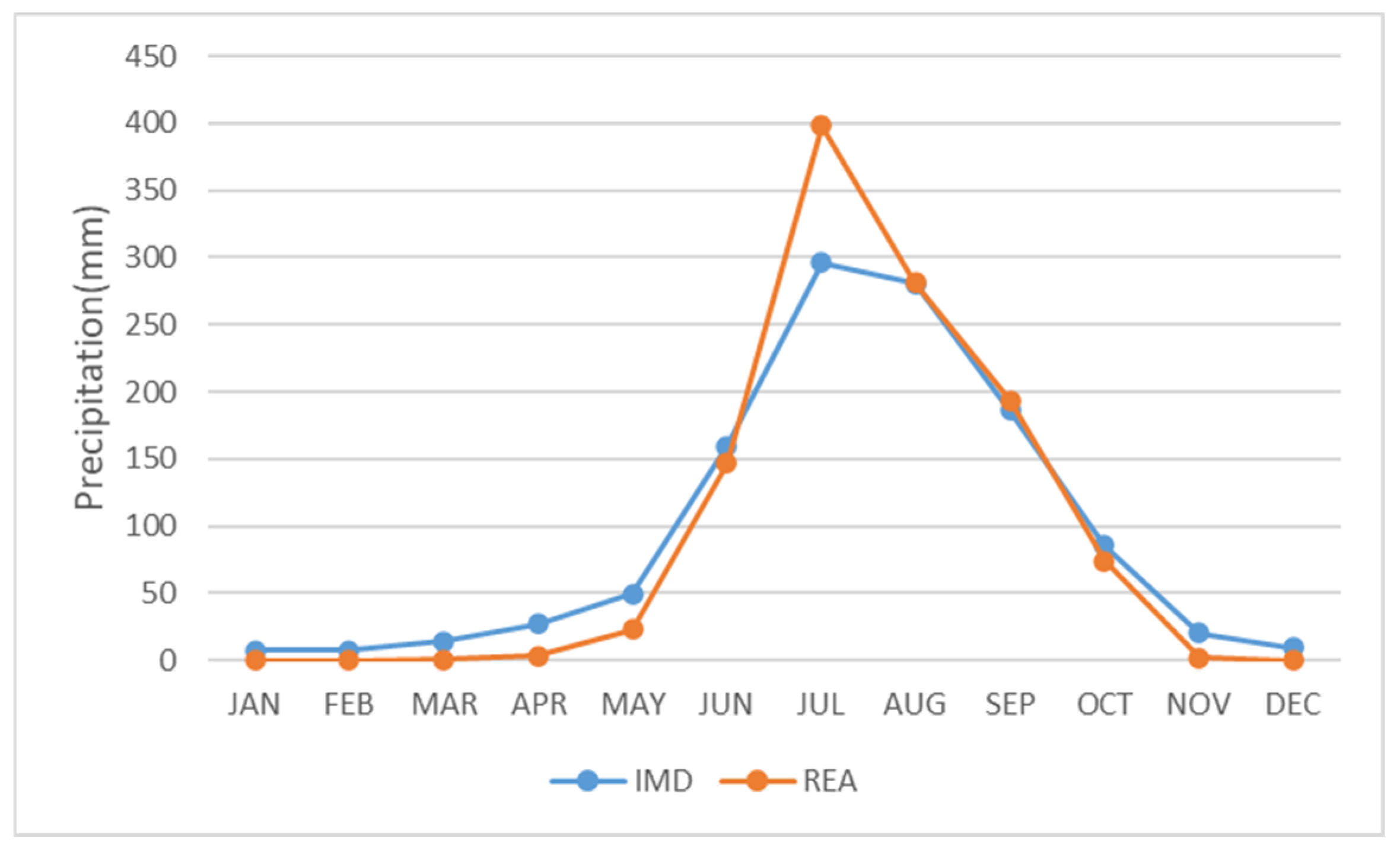
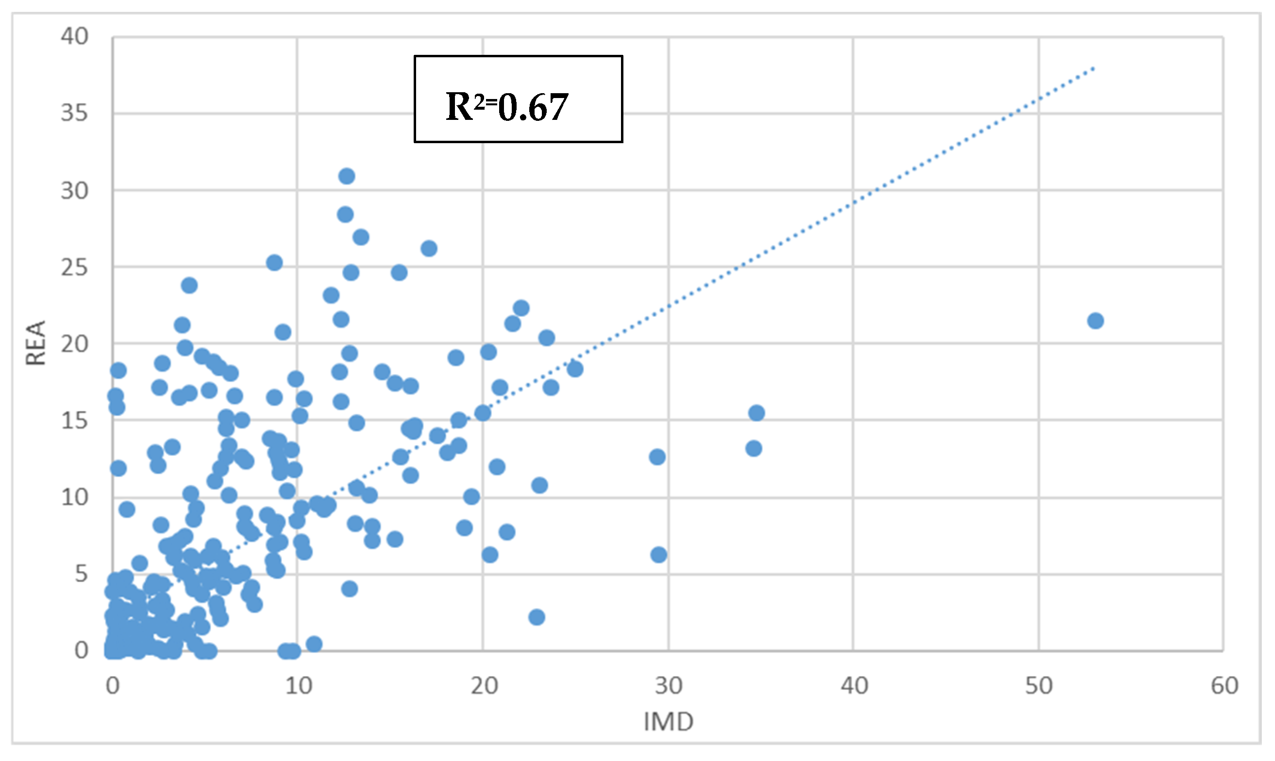
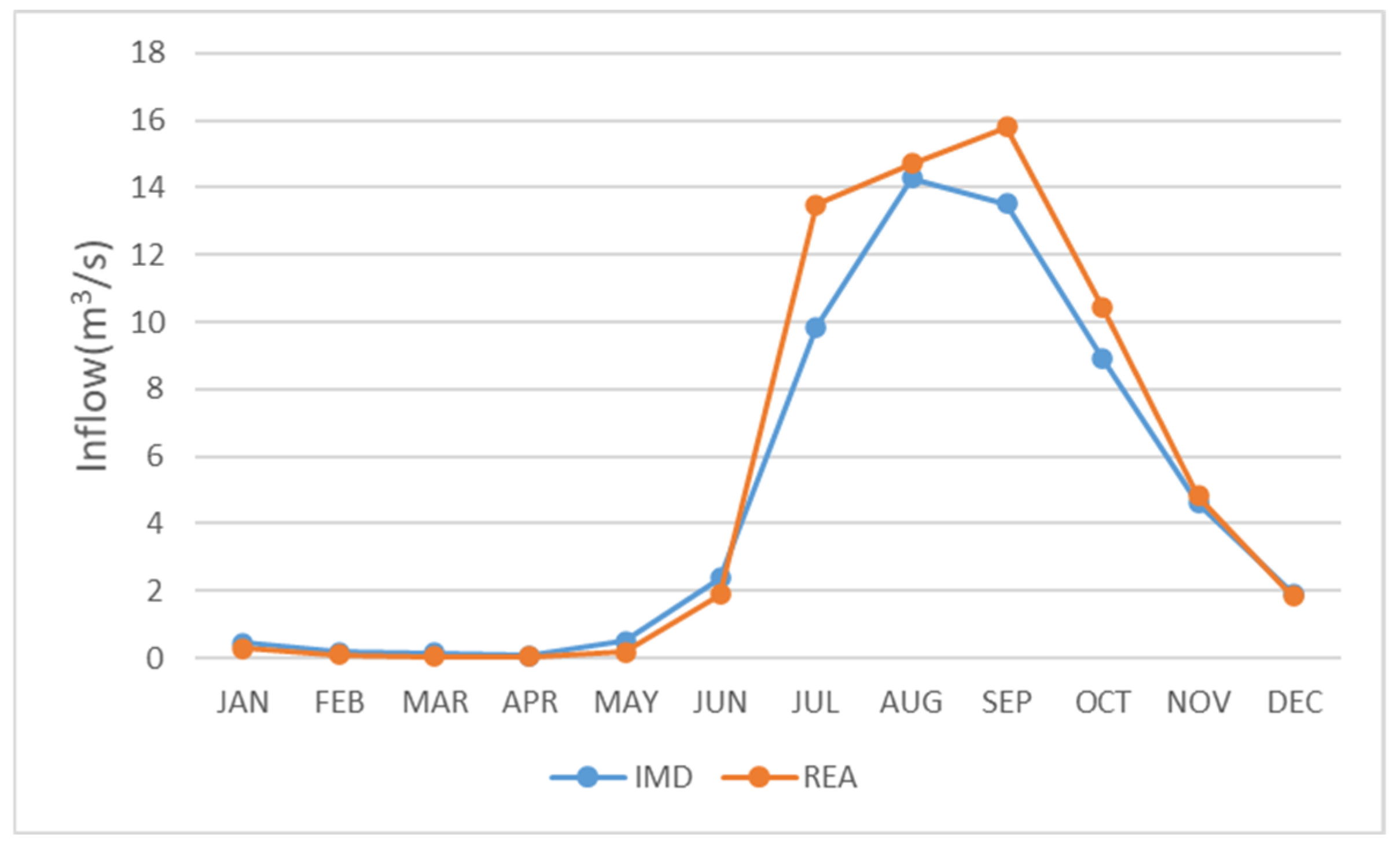
3.1. Climate Variables from REA_QM

The hydrologic components of the Pakhal Watershed were simulated using the calibrated and validated SWAT model for historic (1988–2018) and future (2021–2050) periods using an REA ensemble of 21 NEX-GDDP models. For the analysis of climate change, the simulated hydrologic conditions are compared to the observed data at each grid point level. The precipitation and temperature from 21 NEX-GDDP models are compared with the IMD data to determine the correlation. It was observed that the R² values for the climate variables were found to be less than 0.5, indicating that none of the models have a good correlation with the observed data. In order to account for model uncertainty, the REA_QM method is performed to obtain an ensemble model for both historic and future time periods.

Table 2. REA weights for the three climate variables for two climate scenarios at grid 18.785, 78.375.

	Precipitation			Maximum Temperature			Minimum Temperature
Model	Historic	RCP 4.5	RCP 8.5	Historic	RCP 4.5	RCP 8.5	Historic	RCP 4.5	RCP 8.5
ACCESS1-0	0.0848	0.0379	0.0091	0.0531	0.0470	0.0454	0.0356	0.0480	0.0480
BCC-CSM1-1	0.0229	0.0527	0.0575	0.0437	0.0482	0.0475	0.0438	0.0469	0.0469
BNU-ESM	0.0272	0.0560	0.0612	0.0492	0.0481	0.0483	0.0398	0.0484	0.0484
CanESM2	0.0166	0.0640	0.0424	0.0392	0.0479	0.0472	0.0332	0.0472	0.0472
CCSM4	0.0309	0.0355	0.0480	0.0542	0.0472	0.0475	0.0576	0.0483	0.0483
CESM1-BGC	0.1612	0.0543	0.0255	0.0409	0.0466	0.0454	0.0427	0.0449	0.0449
CNRM-CM5	0.0403	0.0390	0.0427	0.0508	0.0480	0.0486	0.0439	0.0483	0.0482
CSIRO-Mk3-6-0	0.0322	0.0360	0.0353	0.0541	0.0484	0.0487	0.0799	0.0486	0.0485
GFDL-CM3	0.0311	0.0424	0.0420	0.0445	0.0473	0.0483	0.0592	0.0468	0.0468
GFDL-ESM2G	0.0362	0.0439	0.0555	0.0525	0.0494	0.0486	0.0420	0.0498	0.0498
GFDL-ESM2M	0.1678	0.0361	0.0450	0.0413	0.0477	0.0483	0.0408	0.0479	0.0479
INMCM4	0.0613	0.0467	0.0330	0.0518	0.0485	0.0479	0.0703	0.0490	0.0491
IPSL-CM5A-LR	0.0281	0.0535	0.0613	0.0426	0.0478	0.0476	0.0498	0.0493	0.0493
IPSL-CM5A-MR	0.0400	0.0392	0.0493	0.0462	0.0474	0.0484	0.0365	0.0482	0.0481
MIROC5	0.0285	0.0441	0.0657	0.0473	0.0478	0.0485	0.0719	0.0475	0.0475
MIROCESM	0.0222	0.0740	0.0786	0.0452	0.0473	0.0474	0.0363	0.0470	0.0471
MIROCHEM	0.0285	0.0572	0.0720	0.0459	0.0473	0.0473	0.0297	0.0467	0.0467
MPI-ESM-LR	0.0328	0.0454	0.0312	0.0502	0.0469	0.0473	0.0415	0.0464	0.0464
MPI-ESM-MR	0.0220	0.0499	0.0412	0.0535	0.0472	0.0464	0.0348	0.0462	0.0462
MRI-CGCM3	0.0637	0.0411	0.0456	0.0478	0.0471	0.0477	0.0612	0.0469	0.0469
NorESM1-M	0.0219	0.0511	0.0578	0.0460	0.0468	0.0477	0.0497	0.0478	0.0478

shows the REA ensemble initial (historic) and final weights (future) for the climate models corresponding to each climate variable. The weights for each grid point are shown in Table 2. The same procedure is applied for all of the grid points in the study area. The obtained weights are applied to the climate data and REA mean is calculated for each climate variable and then used for SWAT model simulation after performing bias correction using QM. The bias correction results obtained using the QM method are given in the Supplementary Material (Figure S2).

The scatter plot for REA and IMD monthly precipitation is shown in Figure 3. It is seen that the REA model has a good match with the observed data, with a correlation coefficient (R²) of 0.74. The average monthly precipitation from REA and IMD is shown in Figure 4. The R² value for REA temperature and observed temperature are 0.94 and 0.96 for maximum and minimum temperature, respectively. The scatter plot for monthly streamflow (tank inflow) with REA and IMD as input are shown in Figure 5. It seen that the REA model has a good fit to the observed data with a value of R² as 0.67. The average monthly precipitation from REA and IMD is shown in Figure 6. The REA model monthly streamflow is comparable to IMD data.

3.2. Historic and Future NEX-GDDP Climate Data Analysis

Table 3. Change in NEX-GDDP simulated climate variables compared to observed data.

Period	P (mm)	ΔP (%)	SF	ΔSF (%)	Tmax (°C)	ΔTmax	Tmin (°C)	ΔTmin	ET (mm)	ΔET (%)
IMD	1143.04		56.76		33.42		22.07		595.66
1988–2018
Historic	1120.81	−1.95	63.63	12.10	33.35	−0.07	22.10	0.03	510.55	−14.29
1988–2018
Future RCP4.5	1020.25	−10.74	54.99	−3.12	34.63	1.21	23.29	1.22	511.62	−14.11
2021–2050
Future RCP8.5	1178.94	3.14	68.53	20.73	34.84	1.42	23.55	1.48	517.63	−13.10
2021–2051

depicts the changes in NEX-GDDP hydroclimatic variables with respect to observed data under historic and future time periods. It is observed that precipitation is under predicted by 2% in the past. While the streamflow is over predicted by 12% during the historic period. The streamflow over prediction can be attributed to the changes in minimum and maximum temperatures. When compared to observation data under RCP 4.5, both precipitation and streamflow are reduced in the future (2021–2050). Precipitation and streamflow, on the other hand, show an increasing trend under the RCP 8.5 scenario. They are similar to observed data during the historical period. In future period, under the RCP 4.5 scenario both the maximum and minimum temperatures increased by 1.21 °C and 1.22 °C, respectively. Under RCP 8.5, the changes are 1.42 °C and 1.48 °C for minimum and maximum temperatures, respectively. The changes in evapotranspiration showed a decreasing trend in both future RCP scenarios.

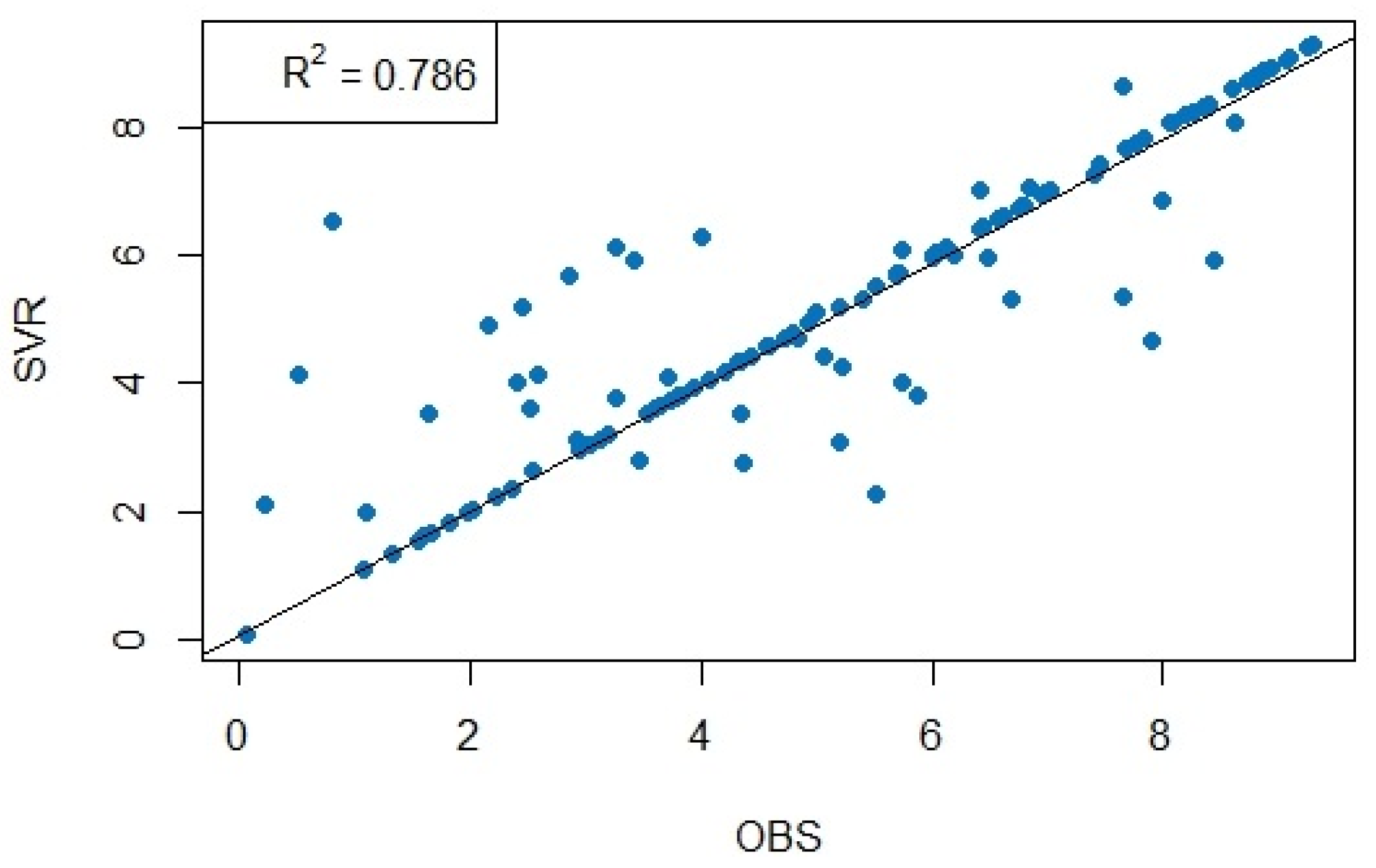
3.3. Performance of the ν-SVR Model

The parameter combination of C = 34, v = 0.5, γ = 0.91 with the radial basis kernel function produced the best match between the predicted and observed water level change (Figure 7). The R² value was 0.79, MAE was 0.018 m, and RMSE was 0.13 m for the training period. The scatter plot between the observed and SVR model generated tank water levels during the training period is shown in Figure 8. In the validation period, the R², MAE and RMSE values changed slightly to 0.72, 0.6 m and 0.25 m, respectively. The scores of the three metrics (R, MAE and RMSE) during the training and validation periods suggest that the model performance is satisfactory in capturing the observed lake water level trends. The time series plot of observed and SVR model monthly lake water level changes suggests that the model performance is good (Figure 9).

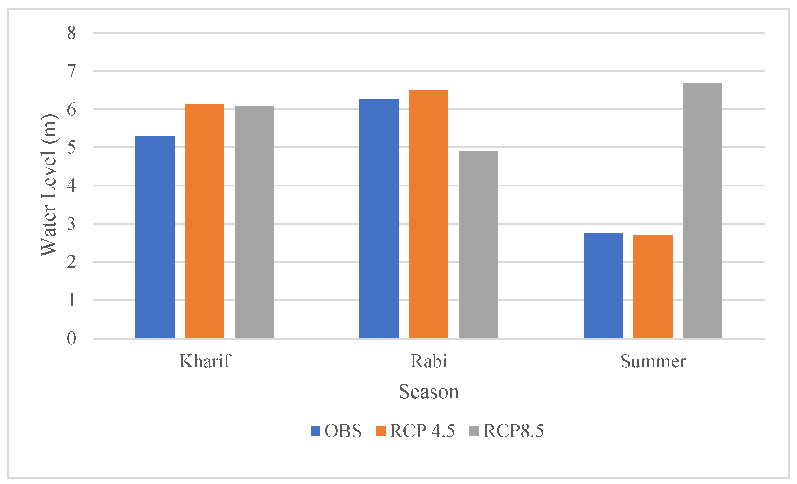
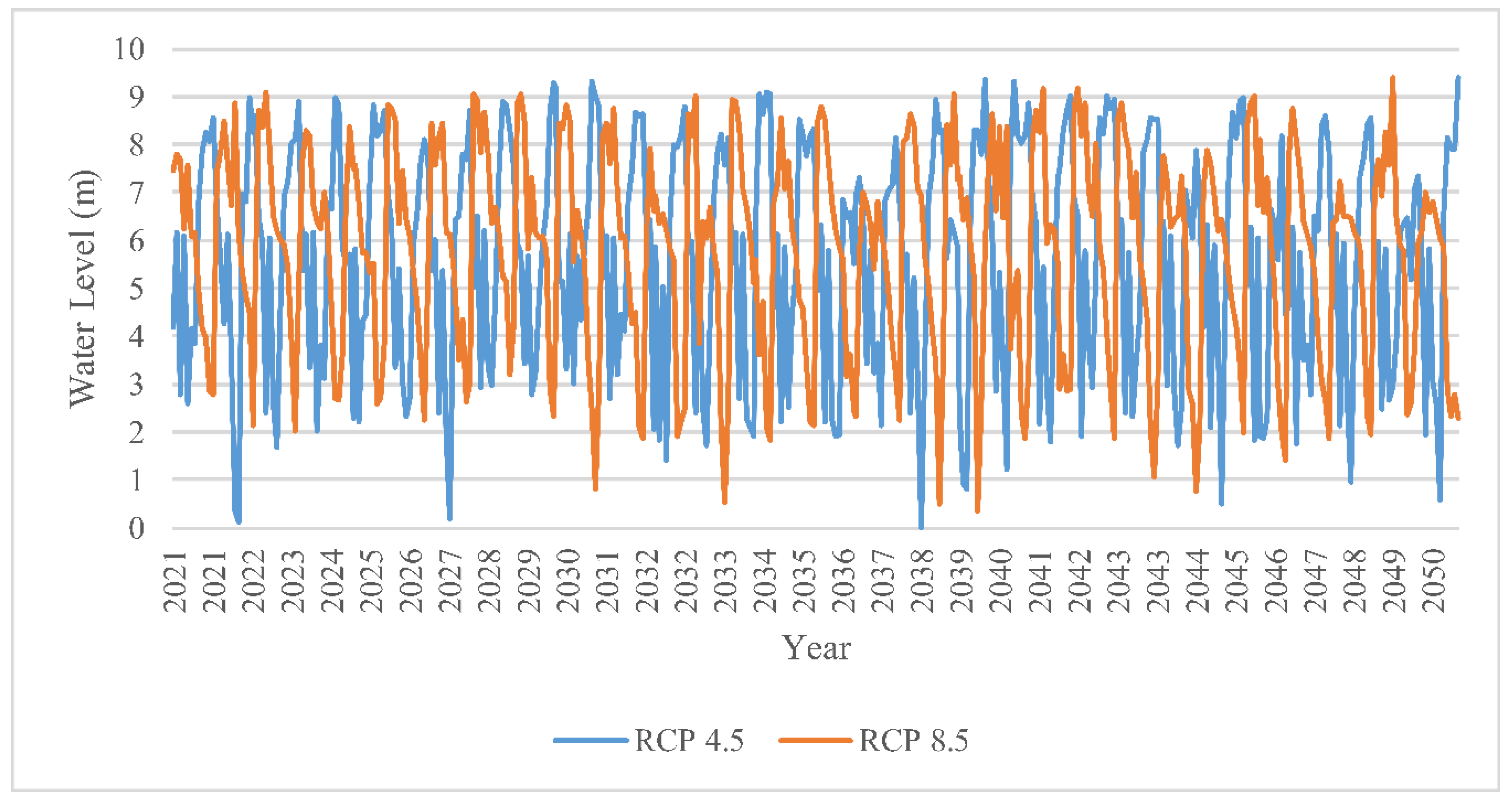
3.4. Effect of Climate Change on Water Availability

The calibrated and validated SVR model is used to make monthly tank water level predictions under RCP 4.5 and RCP 8.5 scenarios for the period 2021–2050. The changes in predicted monthly lake water level is shown in Figure 10. The lake water level ranges during the observation period (2003–2018) are 0.05–9.3 m. The future lake water level ranges under RCP 4.5 and RCP 8.5 are 0.0–9.2 m, 0.35–9.8 m, respectively. The average water level observed during the SVR modeling period (2003–2018) is 5.2 m. Whereas, the average water level range during future scenarios was between 5.6 m and 5.8 m under both RCPs. The average lake water levels for the future scenarios are similar to the historic trends.

Seasonal analysis is performed in order to assess the changes in water levels during rabi and kharif seasons. Three crop growth seasons are considered for the analysis are rabi (July–October), kharif (October–April) and summer (May–June). The average changes in water levels during each season are shown in Figure 11. The results under RCP 4.5 signify an increase water levels in rabi and kharif season, while a decrease in water levels in summer season. Under RCP 8.5, the water levels showed an increase in water elevels in Kharif while a significant decrease in levels can be in the rabi season. High increase in water levels can be observed in Summer under RCP 8.5. These changes can be attributed to changes in the climate variables.

4. Discussion

In the current study, the NEX-GDDP climate data is preprocessed first, and then an ensemble model is generated using the REA QM method. The REA method utilizes all 21 of the models in the dataset. The approach uses weights for both historical and future time periods. The weights obtained for the historical time period are known as initial weights, and they determine the model’s reliability in representing the observed data. The initial weights for precipitation range from 0.016 to 0.167, indicating that none of the models is reliable in capturing the observed precipitation profiles. The REA method effectively accounts for model uncertainty on future projections by providing different sets of weights for each RCP scenario. Although the NEX-GDDP dataset is a bias-corrected product, significant biases were discovered when the climate parameters from the ensemble model were compared to the observed data for the study area (IMD data). The quantile mapping bias correction method is used to account for the biases in the ensemble model. The results of the QM method, as shown in Figure S1, indicate that the QM method is effective in eliminating biases.

The climate variables from the ensemble model are used in the SWAT model to predict the future water balancing components in the Phakal lake catchment. The results show that the RCP 4.5 is vulnerable to climate change due to a decrease in precipitation and streamflow. In comparison, the RCP 8.5 scenario results show an increase in precipitation and streamflow. Temperature and evapotranspiration changes are comparable in both RCP scenarios. The results are consistent with previous literature [52]. The linking of SWAT outputs with the SVR model proved effective in predicting lake water levels because the performance metrics are satisfactory. When compared to observed levels, predicted lake water levels show a similar pattern under both climate scenarios. The findings indicate that lake level fluctuations are highly dependent on evapotranspiration in the lake catchment. More research is needed to correlate the catchment water balance components and lake levels on a monthly and seasonal scale. The monthly water level results in both RCP 4.5 and 8.5 show nearly zero values in some cases (Figure 9). As a result, research into extreme event analysis is required in order to identify events in which the lake dries up completely.

5. Conclusions

In the present study, an integrated approach of linking SWAT model outputs with support vector regression (v-SVR) has been developed for the prediction of future lake water levels of a tank located in a semi-arid region. Realiability Ensemble Averaging paired with Quantile mapping (REA_QM) method is used for 21 NEX-GDDP climate model data, in order to obtain a single reliable ensemble future climate model data under both RCP 4.5 and 8.5 scenarios. These climate datasets are used as input in future water level prediction of Pakhal Lake. The key findings of the study are as follows: (1) The climate variables obtained from REA_QM method have a high correlation with observed data, (2) the outcomes of both future climate scenarios are different. A decrease in streamflow is obeserved in RCP 4.5 which can be attributed to decreased precipitation and enhanced potential evapotranspiration (PET). An increased streamflow is predicted in RCP 8.5, and (3) precipitation, outflow volume, PET and inflows from SWAT can be used as input variables in SVR to estimate lake water level when direct estimation of surface evaporation from the lake is not possible. This method can be an effective way for estimating water levels, since the changes in future lake area information is unavailable, (4) The predicted lake water levels indicate a similar pattern under both the climate scenarios when compared to observed levels. Seasonal analysis suggests a decrease in water availability in the rabi season under RCP 8.5 scenario. Significant extreme events are observed in the RCP 4.5 scenario. As majority of the lake waters are used for agricultural purpose, adaptation strategies are required for sustainable management of water resources. This study aids in planning necessary water management options of Pakhal Lake in the face of changing climate. The seasonal analysis aids in developing policies for water augmentation from the lake linking project in order to sustain agriculture during periods of water scarcity. The methodology developed in the present study can be extended to other semi-arid lake systems with limited observed data.

References

1. Kwarteng, E.A.; Gyamfi, C.; Anyemedu, F.O.K.; Adjei, K.A.; Anornu, G.K. Coupling SWAT and Bathymetric Data in Modelling Reservoir Catchment Hydrology. Spat. Inf. Res. 2021, 29, 55–69. [Google Scholar] [CrossRef]
2. Chen, Y.D.; Chen, X.; Xu, C.-Y.; Shao, Q. Downscaling of Daily Precipitation with a Stochastic Weather Generator for the Subtropical Region in South China. Hydrol. Earth Syst. Sci. Discuss. 2006, 3, 1145–1183. [Google Scholar] [CrossRef]
3. Qin, X.S.; Huang, G.H.; Chakma, A.; Nie, X.H.; Lin, Q.G. A MCDM-Based Expert System for Climate-Change Impact Assessment and Adaptation Planning—A Case Study for the Georgia Basin, Canada. Expert Syst. Appl. 2008, 34, 2164–2179. [Google Scholar] [CrossRef]
4. Das, J.; Umamahesh, N.V. Assessment of Uncertainty in Estimating Future Flood Return Levels under Climate Change. Nat. Hazards 2018, 93, 109–124. [Google Scholar] [CrossRef]
5. Lenderink, G.; Buishand, A.; Van Deursen, W. Estimates of Future Discharges of the River Rhine Using Two Scenario Methodologies: Direct versus Delta Approach. Hydrol. Earth Syst. Sci. 2007, 11, 1145–1159. [Google Scholar] [CrossRef]
6. Mohammed, R.; Scholz, M. Adaptation Strategy to Mitigate the Impact of Climate Change on Water Resources in Arid and Semi-Arid Regions: A Case Study. Water Resour. Manag. 2017, 31, 3557–3573. [Google Scholar] [CrossRef] [Green Version]
7. Sowjanya, P.N.; Reddy, V.K.; Shashi, M. Intra- and Interannual Streamflow Variations of Wardha Watershed under Changing Climate. ISH J. Hydraul. Eng. 2018, 26, 197–208. [Google Scholar] [CrossRef]
8. Ramabrahmam, K.; Keesara, V.R.; Srinivasan, R.; Pratap, D.; Sridhar, V. Flow Simulation and Storage Assessment in an Ungauged Irrigation Tank Cascade System Using the SWAT Model. Sustainability 2021, 13, 13158. [Google Scholar] [CrossRef]
9. Buri, E.S.; Keesara, V.R.; Loukika, K.N. Spatio-Temporal Analysis of Climatic Variables in the Munneru River Basin, India, Using NEX-GDDP Data and the REA Approach. Sustainability 2022, 14, 1715. [Google Scholar] [CrossRef]
10. Güntner, A.; Krol, M.S.; De Araújo, J.C.; Bronstert, A. Simple Water Balance Modelling of Surface Reservoir Systems in a Large Data-Scarce Semiarid Region/Modélisation Simple Du Bilan Hydrologique de Systèmes de Réservoirs de Surface Dans Une Grande Région Semi-Aride Pauvre En Données. Hydrol. Sci. J. 2004, 49, 37–41. [Google Scholar] [CrossRef]
11. Huang, J.; Ji, M.; Xie, Y.; Wang, S.; He, Y.; Ran, J. Global Semi-Arid Climate Change over Last 60 Years. Clim. Dyn. 2016, 46, 1131–1150. [Google Scholar] [CrossRef] [Green Version]
12. Ge, Y.; Li, X.; Huang, C.; Nan, Z. A Decision Support System for Irrigation Water Allocation along the Middle Reaches of the Heihe River Basin, Northwest China. Environ. Model. Softw. 2013, 47, 182–192. [Google Scholar] [CrossRef]
13. Jayanthi, S.L.S.V.; Keesara, V.R. Climate Change Impact on Water Resources of Medium Irrigation Tank. ISH J. Hydraul. Eng. 2019, 27, 322–333. [Google Scholar] [CrossRef]
14. Dong, H.; Song, Y.; Zhang, M. Hydrological Trend of Qinghai Lake over the Last 60 Years: Driven by Climate Variations or Human Activities? J. Water Clim. Chang. 2018, 10, 524–534. [Google Scholar] [CrossRef]
15. Wang, Z.; Ficklin, D.L.; Zhang, Y.; Zhang, M. Impact of Climate Change on Streamflow in the Arid Shiyang River Basin of Northwest China. Hydrol. Processes 2012, 26, 2733–2744. [Google Scholar] [CrossRef]
16. Palanisami, K.; Meinzen-Dick, R.; Giordano, M. Climate Change and Water Supplies: Options for Sustaining Tank Irrigation Potential in India. Econ. Political Wkly. 2010, 45, 183–190. [Google Scholar]
17. Sanchez-Cohen, I.; Díaz-Padilla, G.; Velasquez-Valle, M.; Slack, D.C.; Heilman, P.; Pedroza-Sandoval, A. A Decision Support System for Rainfed Agricultural Areas of Mexico. Comput. Electron. Agric. 2015, 114, 178–188. [Google Scholar] [CrossRef]
18. Lin, P.; Yang, Z.L.; Cai, X.; David, C.H. Development and Evaluation of a Physically-Based Lake Level Model for Water Resource Management: A Case Study for Lake Buchanan, Texas. J. Hydrol. Reg. Stud. 2015, 4, 661–674. [Google Scholar] [CrossRef] [Green Version]
19. Davraz, A.; Sener, E.; Sener, S. Evaluation of Climate and Human Effects on the Hydrology and Water Quality of Burdur Lake, Turkey. J. Afr. Earth Sci. 2019, 158, 103569. [Google Scholar] [CrossRef]
20. Rani, S.; Sreekesh, S. Evaluating the Responses of Streamflow under Future Climate Change Scenarios in a Western Indian Himalaya Watershed. Environ. Processes 2019, 6, 155–174. [Google Scholar] [CrossRef]
21. Chien, H.; Yeh, P.J.F.; Knouft, J.H. Modeling the Potential Impacts of Climate Change on Streamflow in Agricultural Watersheds of the Midwestern United States. J. Hydrol. 2013, 491, 73–88. [Google Scholar] [CrossRef]
22. Rocha, J.; Carvalho-Santos, C.; Diogo, P.; Beça, P.; Keizer, J.J.; Nunes, J.P. Impacts of Climate Change on Reservoir Water Availability, Quality and Irrigation Needs in a Water Scarce Mediterranean Region (Southern Portugal). Sci. Total Environ. 2020, 736, 139477. [Google Scholar] [CrossRef]
23. Gosain, A.K.; Rao, S.; Arora, A. Climate Change Impact Assessment of Water Resources of India. Curr. Sci. 2011, 101, 356–371. [Google Scholar]
24. Musie, M.; Sen, S.; Srivastava, P. Application of CORDEX-AFRICA and NEX-GDDP Datasets for Hydrologic Projections under Climate Change in Lake Ziway Sub-Basin, Ethiopia. J. Hydrol. Reg. Stud. 2020, 31, 100721. [Google Scholar] [CrossRef]
25. Abbaspour, K.C.; Faramarzi, M.; Ghasemi, S.S.; Yang, H. Assessing the Impact of Climate Change on Water Resources in Iran. Water Resour. Res. 2009, 45, 1–16. [Google Scholar] [CrossRef] [Green Version]
26. Pandey, B.K.; Gosain, A.K.; Paul, G.; Khare, D. Climate Change Impact Assessment on Hydrology of a Small Watershed Using Semi-Distributed Model. Appl. Water Sci. 2017, 7, 2029–2041. [Google Scholar] [CrossRef] [Green Version]
27. Narsimlu, B.; Gosain, A.K.; Chahar, B.R. Assessment of Future Climate Change Impacts on Water Resources of Upper Sind River Basin, India Using SWAT Model. Water Resour. Manag. 2013, 27, 3647–3662. [Google Scholar] [CrossRef]
28. Moriasi, D.N.; Arnold, J.G.; Van Liew, M.W.; Bingner, R.L.; Harmel, R.D.; Veith, T.L. Model Evaluation Guidelines for Systematic Quantification of Accuracy in Watershed Simulations. Trans. ASABE 2007, 50, 885–900. [Google Scholar] [CrossRef]
29. Gassman, P.W.; Reyes, M.R.; Green, C.H.; Arnold, J.G. The Soil and Water Assessment Tool: Historical Development, Applications, and Future Research Directions. Trans. ASABE 2007, 50, 1211–1250. [Google Scholar] [CrossRef] [Green Version]
30. Neitsch, S.L.; Arnold, J.G.; Kiniry, J.R.; Srinivasan, R.; Williams, J.R. Soil and Water Assessment Tool User’s Manual; TWRI Report TR-192; Texas Water Resources Institute, USDA Agricultural Research Service: College Station, TX, USA, 2002; Volume 202, p. 412. [Google Scholar]
31. Gosain, A.K.; Rao, S.; Basuray, D. Special section: Climate change and india climate change impact assessment on hydrology of indian river basins. Curr. Sci. 2006, 90, 346–353. [Google Scholar]
32. Yin, Z.; Feng, Q.; Zou, S.; Yang, L. Assessing Variation in Water Balance Components in Mountainous Inland River Basin Experiencing Climate Change. Water 2016, 8, 472. [Google Scholar] [CrossRef] [Green Version]
33. Uniyal, B.; Jha, M.K.; Verma, A.K. Assessing Climate Change Impact on Water Balance Components of a River Basin Using SWAT Model. Water Resour. Manag. 2015, 29, 4767–4785. [Google Scholar] [CrossRef]
34. Ficklin, D.L.; Luo, Y.; Luedeling, E.; Zhang, M. Climate Change Sensitivity Assessment of a Highly Agricultural Watershed Using SWAT. J. Hydrol. 2009, 374, 16–29. [Google Scholar] [CrossRef]
35. Khalilian, S.; Shahvari, N. A SWAT Evaluation of the Effects of Climate Change on Renewable Water Resources in Salt Lake Sub-Basin, Iran. AgriEngineering 2018, 1, 44–57. [Google Scholar] [CrossRef]
36. Devia, G.K.; Ganasri, B.P.; Dwarakish, G.S. A Review on Hydrological Models. Aquat. Procedia 2015, 4, 1001–1007. [Google Scholar] [CrossRef]
37. Mehan, S.; Neupane, R.P.; Kumar, S. Coupling of SUFI 2 and SWAT for Improving the Simulation of Streamflow in an Agricultural Watershed of South Dakota. Hydrol. Curr. Res. 2017, 8, 1–11. [Google Scholar] [CrossRef]
38. Saade, J.; Atieh, M.; Ghanimeh, S.; Golmohammadi, G. Modeling Impact of Climate Change on Surface Water Availability Using Swat Model in a Semi-Arid Basin: Case of El Kalb River, Lebanon. Hydrology 2021, 8, 134. [Google Scholar] [CrossRef]
39. Bucak, T.; Trolle, D.; Andersen, H.E.; Thodsen, H.; Erdoğan, Ş.; Levi, E.E.; Filiz, N.; Jeppesen, E.; Beklioğlu, M.; Bucak, T. Future Water Availability in the Largest Freshwater Mediterranean Lake Is at Great Risk as Evidenced from Simulations with the SWAT Model. Sci. Total Environ. 2017, 581–582, 413–425. [Google Scholar] [CrossRef]
40. Kisi, O.; Shiri, J.; Karimi, S.; Shamshirband, S.; Motamedi, S.; Petković, D.; Hashim, R. A Survey of Water Level Fluctuation Predicting in Urmia Lake Using Support Vector Machine with Firefly Algorithm. Appl. Math. Comput. 2015, 270, 731–743. [Google Scholar] [CrossRef]
41. Buyukyildiz, M.; Tezel, G.; Yilmaz, V. Estimation of the Change in Lake Water Level by Artificial Intelligence Methods. Water Resour. Manag. 2014, 28, 4747–4763. [Google Scholar] [CrossRef]
42. Mohammadi, B.; Guan, Y.; Aghelpour, P.; Emamgholizadeh, S.; Zolá, R.P.; Zhang, D. Simulation of Titicaca Lake Water Level Fluctuations Using Hybrid Machine Learning Technique Integrated with Grey Wolf Optimizer Algorithm. Water 2020, 12, 3015. [Google Scholar] [CrossRef]
43. Khan, M.S.; Coulibaly, P. Application of Support Vector Machine in Lake Water Level Prediction. J. Hydrol. Eng. 2006, 11, 199–205. [Google Scholar] [CrossRef]
44. Çimen, M.; Kisi, O. Comparison of Two Different Data-Driven Techniques in Modeling Lake Level Fluctuations in Turkey. J. Hydrol. 2009, 378, 253–262. [Google Scholar] [CrossRef]
45. Hipni, A.; El-shafie, A.; Najah, A.; Karim, O.A.; Hussain, A.; Mukhlisin, M. Daily Forecasting of Dam Water Levels: Comparing a Support Vector Machine (SVM) Model With Adaptive Neuro Fuzzy Inference System (ANFIS). Water Resour. Manag. 2013, 27, 3803–3823. [Google Scholar] [CrossRef]
46. TWRIS Dashboard. Available online: https://bhuvan-app1.nrsc.gov.in/twris/geoportal/twris.php?type=Medium&status=Completed&project=Pakhal%20Lake# (accessed on 21 April 2022).
47. Gitau, M.W.; Chaubey, I. Regionalization of SWAT Model Parameters for Use in Ungauged Watersheds. Water 2010, 6, 849–871. [Google Scholar] [CrossRef]
48. Yang, X.; Magnusson, J.; Rizzi, J.; Xu, C.Y. Runoff Prediction in Ungauged Catchments in Norway: Comparison of Regionalization Approaches. Hydrol. Res. 2018, 49, 487–505. [Google Scholar] [CrossRef]
49. Emam, A.R.; Kappas, M.; Hoang, L.; Nguyen, K.; Renchin, T. Hydrological Modeling in an Ungauged Basin of Central Vietnam Using SWAT Model. Hydrol. Earth Syst. Sci. 2016, 44. [Google Scholar] [CrossRef] [Green Version]
50. Thrasher, B.; Maurer, E.P.; McKellar, C.; Duffy, P.B. Technical Note: Bias Correcting Climate Model Simulated Daily Temperature Extremes with Quantile Mapping. Hydrol. Earth Syst. Sci. 2012, 16, 3309–3314. [Google Scholar] [CrossRef] [Green Version]
51. Sajjad, H.; Ghaffar, A. Observed, Simulated and Projected Extreme Climate Indices over Pakistan in Changing Climate. Theor. Appl. Climatol. 2019, 137, 255–281. [Google Scholar] [CrossRef]
52. Nauman, S.; Zulkafli, Z.; Bin Ghazali, A.H.; Yusuf, B. Impact Assessment of Future Climate Change on Streamflows Upstream of Khanpur Dam, Pakistan Using Soil and Water Assessment Tool. Water 2019, 11, 1090. [Google Scholar] [CrossRef] [Green Version]
53. Raghavan, S.V.; Hur, J.; Liong, S.Y. Evaluations of NASA NEX-GDDP Data over Southeast Asia: Present and Future Climates. Clim. Chang. 2018, 148, 503–518. [Google Scholar] [CrossRef]
54. Bao, Y.; Wen, X. Projection of China’s near- and Long-Term Climate in a New High-Resolution Daily Downscaled Dataset NEX-GDDP. J. Meteorol. Res. 2017, 31, 236–249. [Google Scholar] [CrossRef]
55. Pai, D.S.; Sridhar, L.; Rajeevan, M.; Sreejith, O.P.; Satbhai, N.S.; Mukhopadhyay, B. Development of a New High Spatial Resolution (0.25° × 0.25°) Long Period (1901–2010) Daily Gridded Rainfall Data Set over India and Its Comparison with Existing Data Sets over the Region. Mausam 2014, 65, 1–18. [Google Scholar] [CrossRef]
56. Srivastava, A.K.; Rajeevan, M.; Kshirsagar, S.R. Development of a High Resolution Daily Gridded Temperature Data Set (1969–2005) for the Indian Region. Atmos. Sci. Lett. 2009, 10, 249–254. [Google Scholar] [CrossRef]
57. Chen, H.P.; Sun, J.Q.; Li, H.X. Future Changes in Precipitation Extremes over China Using the NEX-GDDP High-Resolution Daily Downscaled Data-Set. Atmos. Ocean. Sci. Lett. 2017, 10, 403–410. [Google Scholar] [CrossRef] [Green Version]
58. Xu, R.; Chen, Y.; Chen, Z. Future Changes of Precipitation over the Han River Basin Using NEX-GDDP Dataset and the SVR_QM Method. Atmosphere 2019, 10, 688. [Google Scholar] [CrossRef] [Green Version]
59. Giorgi, F.; Mearns, L.O. Calculation of Average, Uncertainty Range, and Reliability of Regional Climate Changes from AOGCM Simulations via the “Reliability Ensemble Averaging” (REA) Method. J. Clim. 2002, 15, 1141–1158. [Google Scholar] [CrossRef]
60. Mujumdar, P.P.; Ghosh, S. Modeling GCM and Scenario Uncertainty Using a Possibilistic Approach: Application to the Mahanadi River, India. Water Resour. Res. 2008, 44, 1–15. [Google Scholar] [CrossRef]
61. Xu, Y.; Gao, X.; Giorgi, F. Upgrades to the Reliability Ensemble Averaging Method for Producing Probabilistic Climate-Change Projections. Clim. Res. 2010, 41, 61–81. [Google Scholar] [CrossRef] [Green Version]
62. Chandra, R.; Saha, U.; Mujumdar, P.P. Model and Parameter Uncertainty in IDF Relationships under Climate Change. Adv. Water Resour. 2015, 79, 127–139. [Google Scholar] [CrossRef]
63. Das, J.; Treesa, A.; Umamahesh, N.V. Modelling Impacts of Climate Change on a River Basin: Analysis of Uncertainty Using REA & Possibilistic Approach. Water Resour. Manag. 2018, 32, 4833–4852. [Google Scholar] [CrossRef]
64. Teutschbein, C.; Seibert, J. Bias Correction of Regional Climate Model Simulations for Hydrological Climate-Change Impact Studies: Review and Evaluation of Different Methods. J. Hydrol. 2012, 456–457, 12–29. [Google Scholar] [CrossRef]
65. Fang, G.H.; Yang, J.; Chen, Y.N.; Zammit, C. Comparing Bias Correction Methods in Downscaling Meteorological Variables for a Hydrologic Impact Study in an Arid Area in China. Hydrol. Earth Syst. Sci. 2015, 19, 2547–2559. [Google Scholar] [CrossRef] [Green Version]
66. Ringard, J.; Seyler, F.; Linguet, L. A Quantile Mapping Bias Correction Method Based on Hydroclimatic Classification of the Guiana Shield. Sensors 2017, 17, 1413. [Google Scholar] [CrossRef] [Green Version]
67. Bong, T.; Son, Y.-H.; Yoo, S.-H.; Hwang, S.-W. Nonparametric Quantile Mapping Using the Response Surface Method–Bias Correction of Daily Precipitation. J. Water Clim. Chang. 2017, 9, 525–539. [Google Scholar] [CrossRef]
68. Yang, T.; Asanjan, A.A.; Welles, E.; Gao, X.; Sorooshian, S.; Liu, X. Developing Reservoir Monthly Inflow Forecasts Using Artificial Intelligence and Climate Phenomenon Information. Water Resour. Res. 2017, 53, 2786–2812. [Google Scholar] [CrossRef]
Figure 1. Location map of Pakhal Lake and its catchment and command area.
Sustainability 14 06974 g001
Figure 2. Annual Crop Area Statistics for Phakal Lake (Source: TWRIS-ISRO, 2021 [46]).
Sustainability 14 06974 g002
Figure 3. The scatter plot between REA and IMD monthly precipitation in mm for historic period from 1986 to 2018.
Sustainability 14 06974 g003
Figure 4. Average monthly precipitation for REA model and observed data during the historic period (1986–2018).
Sustainability 14 06974 g004
Figure 5. The scatter plot between monthly streamflow (m3/s) simulated with REA and IMD data for the historic period (1986–2018).
Sustainability 14 06974 g005
Figure 6. Average monthly streamflow simulated with REA model and IMD data during the historic period (1986–2018).
Sustainability 14 06974 g006
Figure 7. Observed and modelled water level changes in the ν—SVR model during the training and validation periods.
Sustainability 14 06974 g007
Figure 8. Scatter Plot between observed and SVR simulated tank water levels during the training period.
Sustainability 14 06974 g008
Figure 9. Observed and SVR model average monthly lake water level changes for the period 2003–2018.
Sustainability 14 06974 g009
Figure 10. Changes in predicted monthly lake water level during 2021–2050 under climate changes scenarios.
Sustainability 14 06974 g010
Figure 11. Changes in water levels during each season compared to observed levels under RCP climate change scenarios.
Sustainability 14 06974 g011