Abstract
Hybrid aerial and ground vehicles are seen as a promising option for deployment in a post-disaster assessment due to the risk of infrastructure damage that may hinder the assessment operation. The efficient operation of the hybrid aerial and ground vehicle, particularly routings, remains a challenge. The present study proposed a collaborative hybrid aerial and ground vehicle to support the operation of post-disaster assessment. The study developed two models, i.e., the Two-Echelon Vehicle Routing Problem combined with Assignment (2EVRPA) and the Two-Echelon Collaborative Vehicle Routing Problem (2ECoVRP) to evaluate optimal routings for both aerial and ground vehicles. The difference lies in the second echelon in which the 2EVRPA uses a single point-to-point assignment, whereas the 2ECoVRP considers the collaborative routings between the ground vehicle and the aerial vehicle. To demonstrate its applicability, the developed models were applied to solve the post-disaster assessment for the Mount Merapi eruption in Yogyakarta, Indonesia. Sets of numerical experiments based on the empirical case were conducted. The findings indicate that the 2ECoVRP performs better than 2EVRPA in terms of the total operation time. The tabu search algorithm was found to be a promising method to solve the models due to its good quality solution and computational efficiency. The deployment of eight drones appears to be optimum for the given network configuration of the studied case. Flight altitude and battery capacity were found to be influential to the operation time, hence requiring further exploration. Other potential avenues for future research are also discussed.
1. Introduction
In humanitarian operations, a faster response is critical to save more human lives and reduce casualties [1]. Due to their quick, flexible, and cheap operation, unmanned aerial vehicles (UAVs), commonly known as drones, are seen as a promising technology to support humanitarian operations, particularly with respect to post-disaster assessment and last-mile delivery for aid. The drone has been widely implemented in diverse applications such as military, agriculture, forestry, geographical surveillance, sports, and entertainment [2,3]. The application of the drone in humanitarian operations is, however, very rare. Nevertheless, there is growing interest to deploy drones in humanitarian operations [4].
Humanitarian operations are characterized by high uncertainty, dynamicity, and the goal of alleviating human suffering/saving human life, implying that time is a critical factor [1]. Typical disasters such as earthquakes, tsunamis, volcano eruptions, and pandemics are unpredictable. They pose challenges on humanitarian operations in which affected areas, infrastructure damage (e.g., roads, bridges), and the number and location of victims are unknown. That uncertainty is increased as the conditions change over time. Although most disasters are barely predictable, several efforts have been conducted to minimize the impacts. For instance, during the preparedness phase, prepositioning inventory, dedicated shelters, and evacuation routes have been pre-arranged [5]. During emergency response (post-disaster), humanitarian operations such as search and rescue missions and aid delivery focus on providing a fast response in an efficient way (due to limited resources). To perform efficient and immediate emergency response, information on the number and location of victims, incurred damage, and logistics capability should be on-hand. Post-disaster assessment to provide accurate and timely required information is therefore necessary. The assessment should be conducted as quickly as possible: the faster the rescue operations can be performed, the more likely the victims are to be rescued. This is also the case for aid delivery. The faster the demands for aids are known, the faster the required aids can be delivered, and consequently, the more likely people will be saved [4]. Another challenge encountered by the post-disaster assessment is the widespread areas needing to be evaluated. Some areas may be inaccessible due to challenging terrain, debris blockage, damaged infrastructure, or other hazards. Resources available for the post-disaster assessment are limited, particularly in developing countries where vehicle resources are quite limited and costly and there are few means of transport. In contrast, drones that are equipped with a high-resolution camera and global positioning system (GPS) modules can provide spatial imaging in a relatively short time and at a low cost. Due to its flexibility and its speed, the drone is particularly useful for post-disaster assessment to collect critical data that are unavailable to the response team. In many cases, disaster-affected areas are inaccessible and unsafe for people. The drone, which is operated remotely, opens new possibilities for inaccessible, hazardous, or cut-off regions. McRae, et al., [6] have demonstrated that drone real-time imagery and GPS coordinates have provided rescuers with valuable information on victim status and location as well as terrain, which allows the rescuers to judiciously plan routes and allocate appropriate resources and personnel. In pandemic situations, drones are useful as transportation modes for delivering aid to reach inaccessible areas [7,8] and reducing the risk of disease spread [9,10]. Furthermore, drones are more efficient in terms of energy consumption/emissions per unit distance than conventional diesel vans [11,12], thus supporting sustainability in humanitarian operations. In light of Sopha, et al., [13], who have highlighted the importance of incorporating sustainability in humanitarian operations to enable long-term solutions, drones contribute toward a more sustainable operation in post-disaster assessment.
Despite the significant role of the drone in humanitarian operations, existing studies addressing this issue are few. Current literature related to the application of drones for humanitarian operations focuses on the technical aspects of drones, such as wireless sensor networks [14], technical evaluation of the effectiveness of the drones [15] and developing image datasets for human detection for search and rescue [4]. In addition to the drones’ technicalities, the operation of the drones such as location, allocation, and routing should also be optimized to support efficient and effective post-disaster assessment. Location addresses where the drones are launched, e.g., at a single depot or multiple depots. Owing to the limited number of drones to perform the post-disaster assessment, the allocated number of drones to each depot is important. The routing of the drones determining the optimal sequence of the area visited by the drones should also be optimized. The present paper, therefore, explores potential models for route planning of the hybrid unmanned aerial and ground vehicles during the post-disaster assessment. Two routing models, i.e., Two-Echelon Vehicle Routing Problem combined with Assignment (2EVRPA) and Two-Echelon Collaborative Vehicle Routing Problem (2ECoVRP) are proposed and contrasted. Post-disaster assessment during the Mount Merapi eruption in Yogyakarta, Indonesia, was used as a studied case to demonstrate the models’ applicability. Tabu search heuristics was developed to solve the medium- and large-scale routing problems.
Because post-disaster assessment should be conducted in widespread areas as quickly as possible, the hybrid aerial and ground vehicle approach should be deployed. Ground vehicles have more capacity and longer operation time than drones. However, ground vehicles are constrained by road network and congestion, consequently having limited accessibility to disaster-affected areas, and they also move more slowly. In contrast, drones can move faster than ground vehicles because the road network is not a constraint. Drones do not experience congestion, and they consume less energy because they are lightweight. However, the drone has a limited operation time due to its battery life. The idea of the hybrid system is basically to take advantage of both vehicles. The typical combination of ground vehicles and drones has been used in commercial last-mile delivery [16,17,18]. Hence, instead of optimizing the drone’s routings, the present study simultaneously optimizes the routings of both the ground vehicle and the drone to globally optimize the assessment operation.
Motivated by the requirement toward practical application of the hybrid ground vehicle and drone operation, the present study developed two models, 2EVRPA and 2ECoVRP, to evaluate optimal routings of both ground vehicle and drone. The first echelon addresses the routing of the ground vehicle, whereas the second echelon addresses the routing of the drone. The 2EVRPA model uses the routing problem in the first echelon and the assignment problem in the second echelon. Unlike the 2EVRP, the 2ECoVRP includes the collaborative operation between the ground vehicle and drone operations (implementing routing problems for both echelons). The 2ECoVRP allows the drone to visit multiple targets in one go in the second echelon.
Some studies using drones in humanitarian operations have existed, such as Mishra, et al., [4], Chowdhury, et al., [19], Cannioto, et al., [20], Oruc and Kara [21], and Luo, et al., [22]. For the hybrid of ground vehicle and drone for post-disaster assessment, Luo, et al., [22] developed the model and tested it through experiments using hypothetical datasets. Otto, et al., [23] indicated that the literature using the combined system of ground vehicle and drone is dominated by experimental and hypothetical studies, in which only 10% were based on the empirical case. In contrast, Asih, et al., [24] demonstrated that the metaheuristics performance applied to hypothetical data is slightly different from that using empirical data. Complementing the previous studies, the present study focuses on the quantitative evaluation of the 2EVRP and its variants. The two proposed models are then implemented in a real/empirical case of post-disaster assessment of the Mount Merapi eruption.
Hence, the present study contributes in two ways. First, the study develops and compares the two models capturing the operational characteristics of post-disaster assessment by introducing the hybrid ground vehicle and drone system. Second, it provides an empirical contribution to evaluating efficient routing strategy for the hybrid ground vehicle and drone in post-disaster assessment for the Mount Merapi eruption.
The paper is structured as follows. This section has highlighted the motivation and the contribution of the paper. Section 2 provides brief reviews of the literature on drone operations, particularly related to the routing problem. Section 3 describes the development of the mathematical models and the solution method, which is followed by the description of the empirical case, the numerical results and analysis, and the practical implications in Section 4. Section 5 concludes and discusses future research.
2. Literature Review
Literature on drones has increased rapidly in recent years and that trend seems likely to continue in the future. The first drone literature was published in 2001 for civil operations dealing with routing problems [23] and was followed by the second publication in 2005 [3]. Since then, the numbers of drone studies were stagnant until 2013, when the body of drone literature began growing dramatically. The development was triggered by Amazon, who had started to develop delivery drones in 2013 [25]. Further, Otto, et al., [23] indicated that more than 75% of the articles have been published in the last seven years. To date, four literature reviews on drone operations exist. Otto, et al., [23] surveyed the optimization approaches for drone operations in civil applications, Khoufi, et al., [26] and Viloria, et al., [3] narrowed the review focusing on the routing aspect including types of problems and resolution methods, and Kellerman, et al., [27] focused on the potential barriers, proposed solutions, and expected benefits of drones for parcel and passenger transportation.
Based on those reviews, drones have been used in diverse applications such as transportation (delivery), communication, logistics processes, surveillance, and monitoring [3]. It is worth noting that drone applications in disaster operations are still very limited, as most drone applications are for commercial delivery. The articles for commercial transportation/delivery applications account for 54% and 41% of the total surveyed articles based on Khoufi, et al., [26] and Viloria, et al., [3], respectively. In contrast, only 3% and 4% of the surveyed articles support disaster operations according to Otto, et al., [23] and Khoufi, et al., [26], respectively. The most recent survey by Viloria, et al., [3] indicated a slight increase of 6% of the articles addressing humanitarian operations, mostly addressing the delivery in humanitarian logistics. Only a few have dealt with post-disaster assessment.
Drones can support various operations such as mapping, monitoring/surveillance, communication, transporting/delivering, and data gathering. Otto, et al., [23] categorized the types of drone operations, which include area coverage (covering location problem), search operations, routing, data gathering and recharging in a wireless sensor network, allocating communication links, and flying wireless ad-hoc networks. Among the surveyed articles, 48% of the articles address routing operation, followed by allocating communication links and area coverage. Only a few papers dealt with routings in disaster operations [23]. A recent study on vehicle routing for post-disaster assessment has been conducted by Bruni, et al., [28], who developed a selective routing problem to minimize the sum of arrival times (total latency) at all nodes.
Concerning routing problems in humanitarian operations, two issues have to be addressed simultaneously: reaching the target and minimizing the operation time. For post-disaster assessment operations when the gathered information depends on the arrival time at the node, the total latency should also be considered. Two classes of routing problems, i.e., the traveling salesman problem (TSP) and the vehicle routing problem, (VRP) have commonly been used in the literature. TSP computes the shortest possible route that visits all targets and returns to the starting position, whereas VRP assigns a set of vehicles that visits all targets in such a way that the routings with the minimum completion time or total operation cost are achieved. According to Viloria, et al., [3], 69% of the surveyed articles consider the routing problem for drones only, whereas 31% introduced the combined system of drones and a ground vehicle. The combined system between the drone and the ground vehicle is motivated by the drone limitations such as limited battery capacity (which constraints operating time) and limited load capacity.
The deployment of the combined system of drone and ground vehicle has accordingly given rise to new variants of TSP and VRP [29]. For a collaborative operation between drone and vehicle, the flying sidekick traveling salesman problem (FSTSP) which determines optimal assignment for a drone working in tandem with a ground vehicle, was developed by Murray and Chu [30]. FS-TSP models the drone that executes an operation to serve targets from the ground vehicle, which traverses at a node, and the drone is retrieved at a rendezvous node. Other TSP variants such as traveling salesman problem with a drone (TSP-D) [31], TSP with multiple drones (TSP-mD) [32], and multiple TSPD (mTSPD) [33] have also been developed. Luo, et al., [34] have further expanded mTSPD to the multi-visit traveling salesman problem with multi-drones (mTSP-mD).
Similarly, the VRP also has many extended variants such as VRP-D, which models a set of ground vehicles equipped with drones to serve the targets [35]. The drone can be launched and picked up at the depot or any of the target nodes. VRPTW-D (vehicle routing problem with time window with a drone) was developed from VRPD by addressing the time window and was even further developed to CVRPTW-D (capacitated vehicle routing problem with time window with a drone) to include payload capacity of drones so that each drone cannot deliver goods exceeding its capacity. Motivated by reducing the number of drones, green vehicle routing problem with drone (GVRP-D) was also proposed by Coelho, et al., [36] and extended to multi-trip vehicle routing problem with drone (MTVRP-D) to embrace the load capacity of drone [37].
The general routing problem (GRP) has also been implemented by Oruc and Kara [21] to deal with routing for post-disaster assessment. Oruc and Kara [21] implemented a bi-objective approach to maximize total value added to assess both road segments (arcs) and population centers (nodes). The GRP differs from VRP in that VRP considers node routing problems, whereas GRP includes both node routing problems (in which assessment targets are located at nodes) and arc routing problems (in which assessment targets are located at arcs on a directed network). As a result, the developed model by Oruc and Kara [21] did not require all nodes or edges to be traversed. Some nodes that lie within the drone’s angular point of view are not visited, and some nodes can be visited more than once.
Another approach, i.e., the two-echelon vehicle routing problem (2EVRP) was developed from the supply chain/logistics field [38]. The 2EVRP is a special case of the two-echelon location routing problem in which the location of all nodes is known. The 2EVRP can be deployed to solve the hybrid aerial and ground vehicle routing by segmenting the system into two echelons. The first echelon refers to the route from starting point (depot) to the stopover point or between stopover points, whereas the second echelon refers to the route from a stopover point to target points. The 2EVRP aims to find a set of first and second echelon routes so that the targets are visited with minimum time/cost. The approach simultaneously optimizes the routes of both a ground vehicle (first echelon) and drones (second echelon). The 2EVRP has been widely used in city logistics/commercial last-mile delivery such as Perboli, et al., [39]. Within the context of humanitarian operations, Luo, et al., [22] have developed the two-echelon ground vehicle and unmanned aerial vehicle routing problem (2E-GU-RP). The difference between the 2E-GU-RP and the developed model in the present study is that the 2E-GU-RP models the drone to be launched at a depot or stopover point and picked up at rendezvous node, whereas 2EVRPA and 2ECoVRP models the drone to be launched and picked up at a stopover point where the drone is launched. Table 1 compares various modeling approaches for the hybrid aerial and ground vehicle.

Table 1.
Modeling approaches for the hybrid aerial and ground vehicle routing.
3. Mathematical Models of the Hybrid Aerial and Ground Vehicle Routing
The 2EVRP is considered a suitable approach to solve the routing problem for post-disaster assessment because the approach allows for more efficient and flexible operations. The approach considers a circumstance when a ground vehicle collaborates with a drone. The 2EVRP can be presented as a two-echelon distribution network. The first echelon considers the ground-space network traveled from a depot to stopover points. The ground vehicle travels on a road network near the reconnaissance area and keeps launching and recycling the drone (first echelon). The second echelon considers the aerial-space network where the drone is launched from the stopover point to the target point(s). The target point is an area where the drone conducts mapping operations and collects the target information and then returns to the ground vehicle before the battery runs out (second echelon).
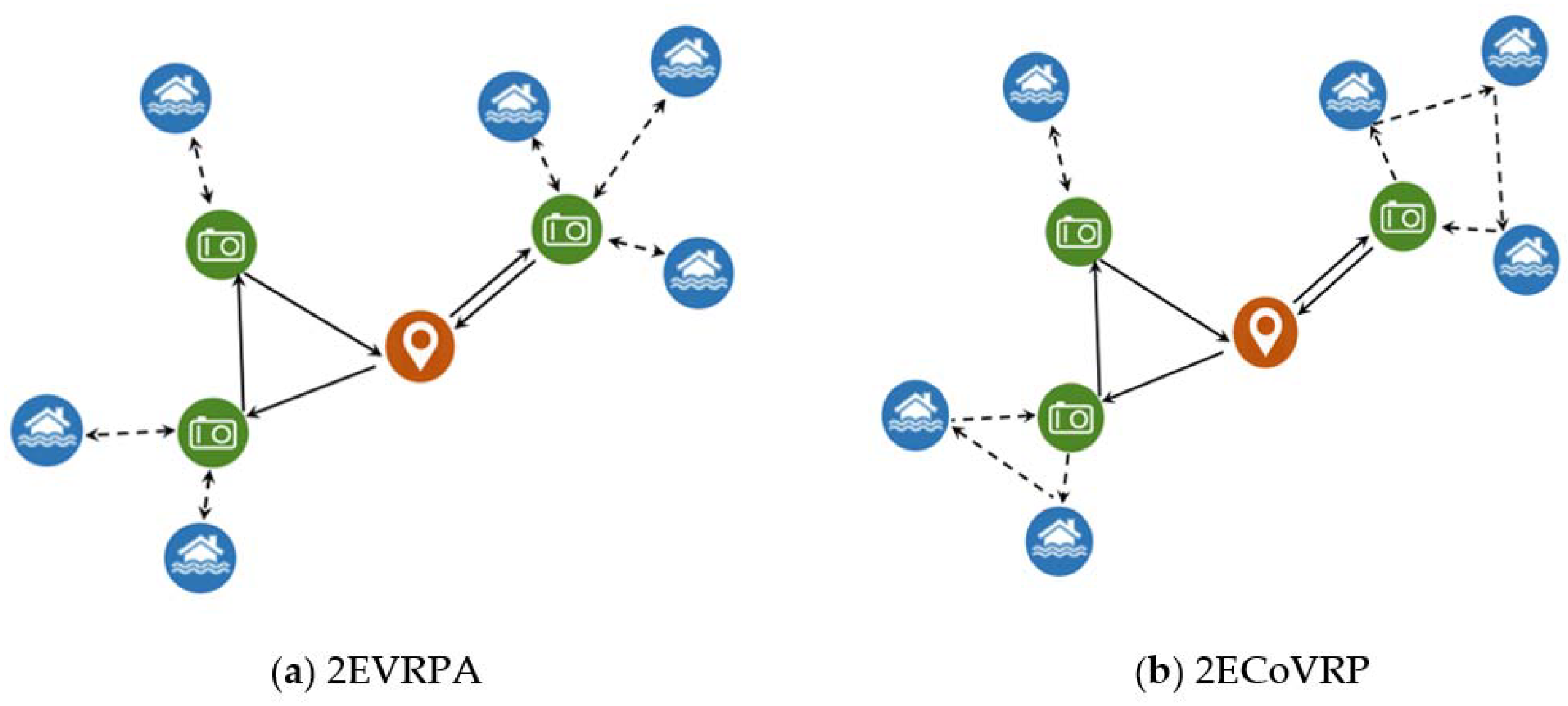
The first variant, the 2EVRPA, applies the routing problem in the first echelon and assignment problem as a sub-problem of the routing problem. The second variant, the 2ECoVRP, includes the collaborative operation between the ground vehicle and drone (implementing routing problems for both echelons). The models allow the drone to visit multiple targets. The schematic diagrams of both the 2EVRPA and the 2ECoVRP are presented in Figure 1.
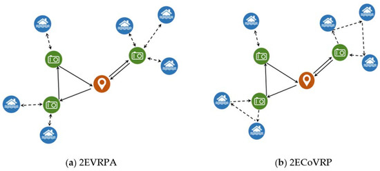
Figure 1.
Schematic diagram: (a) the 2EVRPA, (b) the 2ECoVRP. Note: red dots represent depots, green dots represent stopover points, blue dots represent target points, sold lines represent ground vehicle routing, dashed lines represent drone routing.
3.1. Problem Description and Assumptions
The 2EVRP considers a set of mapping points as targets, each of which must be visited exactly once by a drone. All the mapping points are inaccessible by a ground vehicle. The ground vehicle mounted with a drone departs from a depot and visits stopover points. The drone is launched at the stopover point, visits its mapping point(s), and returns to the launching point to swap its battery for the next flight. The 2EVRPA approach models that once the drone finishes the mapping at the respective target/mapping points, it will return to the launching point although it has still enough battery capacity to perform another mapping process. In contrast, the 2ECoVRP approach allows the drone to visit more than one target/mapping point and will return to the launching point once the battery capacity is insufficient for the next mapping operation. Both models aim to minimize the total operation time for post-disaster assessment.
The assumption used in the models are the following:
- The locations and service times for all mapping points are known;
- All mapping points are visited only once by the drone;
- The locations of the stopover points are known;
- The ground vehicle can only traverse on the road network;
- Each road arc traversed by the ground vehicle corresponds to a flight route of the drone;
- The drone has limited operation time, which is known;
- The time required for battery swap is negligible.
Based on the above description, the notations used in the mathematical models are shown below.
| Sets: | |
| Set of all nodes in the first echelon (includes depot) | |
| Set of all stopover points (without depot) | |
| Set of all mapping points | |
| Set of all vehicles in the first echelon | |
| Parameters: | |
| Travel time of vehicle from gathering point or stopover point to stopover point (includes depot) in the first echelon | |
| Travel time of drone from stopover point to mapping point in the second echelon | |
| Required mapping time for capturing the area of a mapping point | |
| Maximum flight time of the drone | |
| Sufficiently large number | |
| Decision variables | |
| A binary variable that equals one if vehicle v is traveled from node i to j where the edge ; otherwise zero | |
| A binary variable that equals one if the stopover point i is visited where ; otherwise zero | |
| A binary variable that equals one if the drone is traveled from node i to j where the edge ; otherwise zero | |
| The total amount of time needed for drone taking pictures in a stopover point j where | |
| The total amount of time needed for drone traveling in the second echelon where | |
| The total accumulated amount of information gathering time has been used up to stopover point i using vehicle v where and | |
| The total accumulated amount of transportation time has been used up to mapping point i using vehicle v where and | |
3.2. Two-Echelon Vehicle Routing Problem Combined with Assignment (2EVRPA)
The mathematical model of the 2EVRPA was developed based on the basic model of the two-echelon vehicle routing problem (2EVRP) developed by Perboli, et al., [39], which was then modified to facilitate single point-to-point assignment in the second echelon for the present study. A comparable model has been developed for the city logistics context [40]. The 2EVRPA is formulated as the following.
| Objective | ||
| (1) | ||
| Subject to | ||
| (2) | ||
| (3) | ||
| (4) | ||
| (5) | ||
| (6) | ||
| (7) | ||
| (8) | ||
| (9) | ||
| (10) | ||
| (11) | ||
| (12) | ||
| (13) | ||
| (14) | ||
The objective function (1) is to minimize the total operation time, comprising the traveling time of the ground vehicle to carry the drone, the flight time of the drone, and the mapping time of the drone. Constraints (2) and (3) limit that the nodes can only be visited once. Constraint (4) ensures that the vehicle moves consecutively. Constraints (5) and (6) ensure that the ground vehicle returns to the depot once the operation is completed. Constraints (7) and (8) evaluate the total mapping time at each stopover point. Constraints (9) and (10) are used to calculate the traveling time of the drone in the second echelon. Constraint (11) ensures that the mapping point is only visited once by the drone. Constraints (12) and (13) are used for validating the continuity of both ground vehicle’s routes and the drone assignments. Constraint (14) ensures that the drone’s flight time does not exceed the maximum flight time determined by the drone’s battery capacity.
3.3. Two Echelon Collaborative Vehicle Routing Problem (2ECoVRP)
The mathematical model of the 2ECoVRP was constructed by modifying the 2EVRPA model to include the collaborative operation between the ground vehicle and drone operations. The model allows the drone to visit multiple targets in one go (routing problem). The 2ECoVRP model is formulated as below.
| Sets: | ||
| Number of the drone routes in the second echelon | ||
| Decision variables | ||
| A binary variable that equals one if drone route k is traveled from node i to j where the edge ; otherwise zero | ||
| The total amount of time needed for drone mapping in a stopover point j and every routes k where and | ||
| The total amount of time needed for drone traveling in the second echelon where and | ||
| The total amount of time needed for drone traveling in the second echelon where | ||
| The total accumulated amount of transportation time has been used up to mapping point j in route k where and | ||
| The total accumulated amount of information gathering time has been used up at stopover point j in route k where and | ||
| Objective | ||
| (15) | ||
| Subject to | ||
| (16) | ||
| (17) | ||
| (18) | ||
| (19) | ||
| (20) | ||
| (21) | ||
| , | (22) | |
| (23) | ||
| (24) | ||
| (25) | ||
| (26) | ||
| (27) | ||
| (28) | ||
| (29) | ||
| (30) | ||
| (31) | ||
| (32) | ||
| (33) | ||
| (34) | ||
| (35) | ||
| (36) | ||
| (37) | ||
The objective function (15) is to minimize the total operation time consisting of the traveling time of the ground vehicle to carry the drone, the flight time of the drone, and the mapping time of the drone. Constraints (16) and (17) ensure that the nodes can only be visited once. Constraint (18) guarantees that the vehicle moves sequentially. Constraints (19) and (20) ensure that the ground vehicle should return to the depot once the operation is completed. Constraint (21) makes sure all mapping points are visited once, and constraint (22) ensures that the drone visits the mapping points only once. Constraint (23) validates the second echelon vehicle routes and constraint (24) ensures that the drone moves consecutively. Constraint (25) denotes the duration spent at mapping points in the visited route k. Constraint (26) denotes the total accumulated mapping time of each route k. Constraint (27) denotes the accumulated total of mapping time at each stopover point as the accumulated time required to record in that area. Constraint (28) calculates the accumulated mapping time of each mapping point at the stopover point and indicates the stopover point has unlimited capacity. Constraint (29) ensures the total travel time of the drone starts from zero. Constraint (30) ensures the calculation of mapping time starts from zero, and Constraint (31) denotes the mapping duration of the mapping points on each route k, which can be more than zero due to the mapping operation. Constraints (32) and (33) calculate the accumulated travel time of the drone and the total travel time of all drones from the stopover point, respectively. Constraints (34) and (35) are used to validate the continuity of both the ground vehicle’s and the drone’s routing. Constraint (36) validates the mapping process, whereas Constraint (37) limits the flight time of the drone according to its battery capacity, ensuring that it operates below the maximum flight time.
3.4. Tabu Search Algorithm
An optimization problem can be solved by either exact methods or heuristics methods. Exact methods are suitable for solving small-scale problems. However, they may have difficulties in solving a large-scale problem in a reasonable computational time. Heuristics methods, specifically metaheuristics, in contrast, are tailored to find a good solution to large-size and complex problems. Tabu search (TS) is one of the metaheuristics algorithms that was discovered by Glover and formulated in 1989 [41]. Tabu search is an algorithm that incorporates “memory” of the searching history or moves recently applied known as tabu list, which makes it able to search the space economically and effectively. The TS algorithm can avoid the previously visited solution using a tabu list. The tabu list is a short-term set of the solutions, which are changed by the process of moving from one solution to another determined by a set of rules. Despite its adaptive memory, the TS algorithm is also able to accept a worse solution to evade the local optimal trap and can be applied on both discrete and continuous problems. The TS algorithm has been widely used to solve complex problems such as scheduling, quadratic assignment, and routing problems. Several studies, such as Semet and Taillard [42], Chao [43], Scheuerer [44], Boccia, et al., [45], and Venkatachalam, et al., [46], have implemented the tabu search algorithm to solve the two-echelon location-routing problem and the two-echelon routing problem, i.e., truck and trailer routing problem. Furthermore, Venkatachalam, et al., [46] applied the tabu search algorithm to solve the multiple-drone routing problem. It was found that the tabu search algorithm was not only providing a good-quality solution but was also computationally efficient. Similar evidence was also demonstrated by Luo, et al., [34] who solved the multi-visit traveling salesman problem with multi-drones using the tabu search algorithm. The present study thus selects the tabu search algorithm. The tabu search algorithm deployed for the present study is explained in pseudocode as shown in Algorithm 1.
| Algorithm 1. Pseudocode of the proposed tabu search algorithm. |
| Procedure: Tabu Search Input: a set of n neighborhood structure, Nnon-improving, Ncandidate Output: Xbest
|
The algorithm is initiated by constructing an initial solution (Xinit) using a random initial solution and constructing an empty tabu list. Other variables such as current iteration (Iteration = 1) and the number of iterations when the solution is not being improved from the best solution (NonImproveCount = 0) were also initiated. The initial solution is set as the current best solution (Xcurrent) and the best solution found so far (Xbest←Xcurrent←Xinit). At each iteration, a list of candidate solutions (a list of Xnew) is generated by applying a randomly chosen neighborhood n to the current solution (Xcurrent). This procedure is repeated until the number of solutions in the candidate list is equal to Ncandidate. The candidate list is then sorted based on its objective value in ascending order. Subsequently, the algorithm to replace the current solution (Xcurrent) with the new solution from the candidate list (Xnew) is implemented. The algorithm sets rules on the conditions allowing the replacement, i.e., when the new solution is not generated from a tabu move or it is not in the tabu list, and when the new solution passes the aspiration criteria. The aspiration criteria are set based on the condition that the new tabu solution is better than the current solution. Once the new obtained tabu solution is better than the current solution, the new tabu solution will be adopted. Otherwise, it will be taken out from the neighborhood set. The next step is to repeat the checking process of the neighborhood set. The new and the current solution are exchanged and the tabu movement is updated on the tabu list. The previous best-found solution (Xbest) is replaced by the current solution (Xcurrent) once the current solution is better. The count of non-improvement is hence reset (NonImproveCount = 0). However, if the current solution is not better than the best solution, the NonImproveCount is updated. The process is repeated until the termination criteria are met. Otherwise, another iteration for the neighborhood set will be conducted. The proposed TS uses NonImproveCount to decide when the algorithm should be terminated.
4. Computational Results and Analysis
4.1. Case Description: Post-Disaster Assessment for Mount Merapi Eruption
Mount Merapi, the most active volcano in the world, has erupted every four to six years. Within the last 100 years, the largest eruption occurred in 2010, which resulted in 61,154 people being evacuated and 341 casualties [5]. Due to its high occurrence, the regional disaster agency (BPBD–Badan Penanggulangan Bencana Daerah) has formulated a disaster contingency plan, which includes a post-disaster assessment. Due to difficult terrain, the post-disaster assessment becomes challenging. Steep and narrow roads have made some areas inaccessible. However, post-disaster assessment is a crucial operation to support accurate and timely responses.
Therefore, it is necessary to explore an efficient and effective way to support post-disaster assessment. The hybrid ground and aerial vehicle approach seems to be a favorable approach for several reasons. First, the pyroclastic flow of Mount Merapi is barely predictable, making the affected area highly unknown. Second, the pyroclastic flow may emit hazardous and poisonous gas to the surroundings so that it is hazardous for humans. Third, the infrastructure in the affected areas, such as bridges and roads, may be severely damaged, making the areas inaccessible. Using a drone that is mounted on a ground vehicle opens the opportunity to access the disaster-affected areas. Accurate and fast post-disaster assessment is urgently required as the aftermath conditions, such as the number and location of victims and incurred damage of roads and bridges should be known to plan the allocation of resources and personnel as well as to deliver aid efficiently.
Due to the narrow roads and difficult terrain, it appears that motorcycles rather than trucks are the suitable ground vehicles to be deployed for post-disaster assessment for the Mount Merapi eruption. The motorcycle has less carrying capacity than a truck, but the motorcycle has more flexibility to access areas that might be unreachable by truck. The motorcycle brings the drone to map post-disaster conditions. The drone is advantageous for reaching and maneuvering in very narrow terrain such as collapsed buildings. Due to the limited flight time of the drone, the motorcycle increases the mapping coverage. Therefore, the present study uses a motorcycle that is combined with a drone to conduct the post-disaster assessment. The motorcycle is assumed to operate at a constant speed of 45 km/h. The specification for the drones used for the present study is shown in Table 2.
Table 2.
Drone specification.
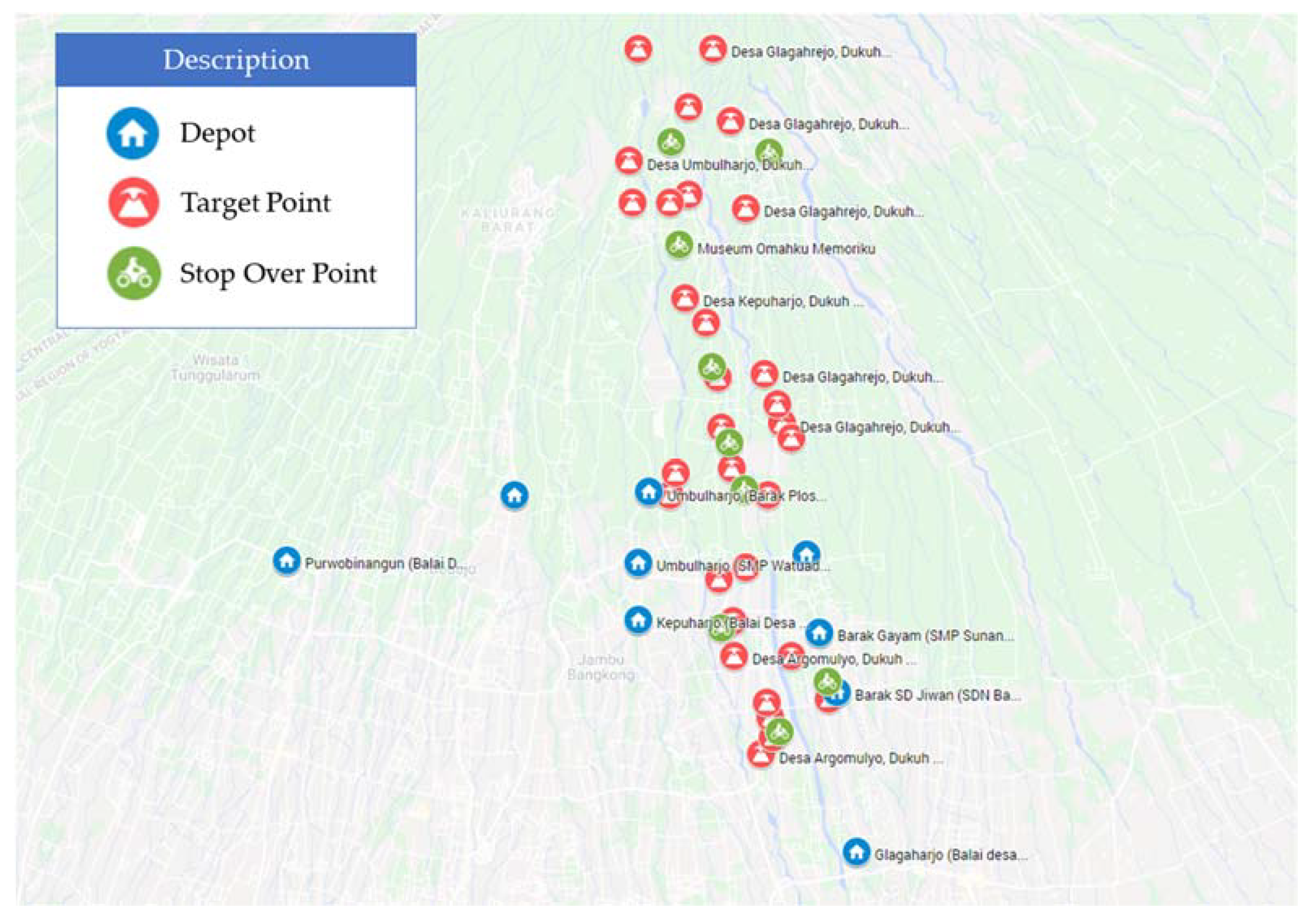
Figure 2 visualizes the network configuration for assessment operation represented by nodes including depots, stopover points, and target/mapping points for post-disaster assessment, which was implemented using Google MyMaps. It includes 49 nodes comprising nine existing depots, 31 target/mapping points, and 9 stopover points. The detailed location in terms of latitude and altitude as well as areas required to be mapped in each target/mapping point is provided in the Appendix A. QGIS was used to measure the time required to travel from one node to another. The area of the target/mapping points was converted into time units, i.e., minutes, by multiplying the area and the mapping rate of 0.00008125 min/m2, as shown in Table 2. The mapping rate was derived from the technical data, indicating the time required by the drones operated at the altitude of 70 m to map the area of 400 m × 400 m is 13 min.
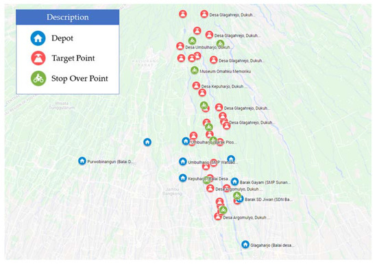
Figure 2.
The affected areas of the Mount Merapi eruption implemented using Google MyMaps with a scale of 1:25,000.
The depots are the starting points of the post-disaster assessment operation. Both motorcycles with mounted drones depart from the depots. The stopover points are the locations where the motorcycles stop and launch the drones for mapping operations. The target/mapping points represent the areas to be mapped by the drones. Each target/mapping point has different areas to be mapped, which then determines the mapping time. The post-disaster assessment operation starts from the depot where the motorcycle that is mounted by a drone is ridden to the stopover points where the drone is launched for mapping. Once the drone nearly reaches the total flight time (running out of its energy), the drone returns to the stopover points. When the mapping operation is accomplished, both the motorcycle and the drone return to the depots. The required total time for those operations is defined as the total operation time.
4.2. Test Instances and Experimental Parameters
To evaluate the consistency of the computational results for various scales, instance benchmarking was conducted. Three groups of instances, based on the procedure developed by Liperda, et al., [47], were conducted. Table 3 presents the three scale categories, i.e., small-, medium-, and large-size instances with various ranges of nodes to have experimented. A set of experiments were conducted for each scale as shown in Table 3. The total conducted computational experiments was 48. Both the results based on individual experiments and average experiments were then reported.
Table 3.
Test instances.
To compare the performance of the E2VRPA and the 2ECoVRP, the values of the objective function (Obj) of both models were contrasted and quantitatively evaluated using Equation (38) as shown below:
To compare the performance of the tabu search algorithm with the exact algorithm, Equations (39) and (40) were used for 2EVRPA and 2ECoVRPA, respectively.
The experiments were conducted using the operational parameters that represent the current conditions (such as the number and location of the depots, the stopover points, mapping/target points, motorcycle speed, and drone specifications). Eight drones with the specification shown in Table 2 were used, each of which was mounted on the motorcycle.
The computational experiments were carried out on a computer with an Intel Core i7-7700 3.6 GHz CPU and 16GB RAM. The model was solved using A Mathematical Programming Language (AMPL) with Gurobi solver using branch and bound method and branch and cut method. A time limit of 6 h (21,600 s) was imposed. The tabu search algorithm was implemented using the C# programming language. The results of the tabu search were reported in terms of the best solution and average solution from ten computational runs for each instance.
The proposed tabu search algorithm used four input parameters: a set of n neighborhood structures, Nnon-improving, Ncandidate, and . A set of n neighborhood structures was used by the algorithm to explore the solution space. The neighborhood operator was selected randomly among neighborhood and N = {Swap, Insert, Reverse}. The proposed tabu search used all of the neighborhoods. The parameter Nnon-improving determined the number of iterations where the best objective function value was not improved consecutively. It was used to terminate the algorithm after it converged to some value in several iterations. The parameter Ncandidate was the number of candidate solutions that were generated at each iteration. The parameter (tabu tenure) was the number of iteration where a move generated by a neighborhood operator was prohibited or considered as a tabu move.
The parameter setting was conducted to help the algorithm provide its best performance in terms of solution quality and computational time. The parameters were set following the procedure known as one factor at a time (OFAT). First, a set of candidate parameters were selected based on previous literature. Second, a preliminary run on the given parameter was conducted to reduce the number of candidates. Finally, the remaining parameters were analyzed iteratively by setting one parameter while the rest of the parameters were fixed. The list of candidate parameters for the final selection was as follows:
Nnon-improving: 25 *|C|*|S|, 50 *|C|*|S|, 100 *|C|*|S|;
Ncandidate: 5, 25, 50;
(tabu tenure): |C|*|S|, 2 *|C|*|S|, 5*|C|*|S|.
The notation |C| and |S| represent the number of nodes in the first echelon (depot and stopover points) and the number of nodes (mapping points) in the second echelon, respectively. The experiment was conducted by selecting three instances, each of which represented small-, medium-, and large-size instances for both the 2EVRPA and the 2ECoVRP. Each instance was solved ten times and the average performance was reported. Figure 3 shows the parameter calibration of the tabu search algorithm. It indicates that the higher value of Nnon-improving led the algorithm to take a longer time for termination. However, there is no significant improvement toward the objective value when changing the value of Nnon-improving from 50 *|C|*|S| to 100 *|C|*|S|. Using a similar approach, the rest of the parameters, i.e., Ncandidate and were analyzed and selected. The selected parameters for the tabu search algorithm were as follows: Nnon-improving = 50 *|C|*|S|, Ncandidate = 25, and = |C|*|S|.
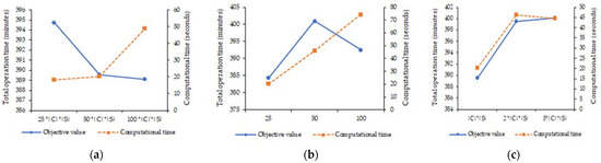
Figure 3.
Parameter settings of the tabu search algorithm: (a) Nnon-improving, (b) Ncandidate, and (c) tabu tenure (θ).
4.3. Performance Comparison of the 2EVRPA and the 2ECoVRP
The performance of the 2EVRPA and the 2ECoVRP in solving the routings of both ground vehicle (i.e., motorcycle) and the drone in the post-disaster assessment of the Mount Merapi eruption was measured using two performance indicators, i.e., the total operation time (which is the value of the objective function) and the computational time to obtain the objective value.
Table 4, Table 5 and Table 6 show the computational results for small-size, medium-size, and large-size instances, respectively. The first column of the tables indicates the identity of the instance. The values of the objective function based on the exact algorithm using AMPL for the 2EVRPA and the 2ECoVRP are reported in the second and the third columns, respectively. Concerning the tabu search algorithm, the values of the best and average objective function for the 2EVRPA are shown in the fourth and fifth columns, whereas those for the 2ECoVRP are shown in the sixth and seventh columns. It is worth noting that for the small-size instances, the comparison evaluation between the 2EVRPA and the 2ECoVRP is based on column 2 (2EVRPA) and column 3 (2ECoVRP). However, for the medium-size and large-size instances, the evaluation is based on column 4 (2EVRPA) and column 6 (2CoVRP) because the exact algorithm cannot obtain optimality. The higher the difference, the better performance of 2ECoVRP compared with that of 2EVRPA. In addition to the objective value, the computational time was also evaluated to measure the efficiency of the two models. The computational times for both the exact algorithm and the tabu search algorithm were also recorded in columns 11–14.
Table 4.
Computational results for small-size instances.
Table 5.
Computational results for medium-size instances.
Table 6.
Computational results for large-size instances.
The findings for small-size instances indicate that the 2ECoVRP performs 14.66% better than the 2EVRPA in terms of the total operation time. However, the 2ECoVRP requires a slightly longer computational time of about five seconds, which is considered insignificant. It is also interesting to highlight that the tabu search algorithm produces results as good as the exact algorithm. The average difference of the total operation time resulting from the tabu search compared to the exact algorithm is 0.34% and 0.30% for the 2EVRPA and the 2ECoVRP, respectively. The average computational time using the tabu search algorithm is about 2.7 s, which is insignificant. The findings imply that the 2ECoVRP approach solved by the tabu search performs reasonably well in small-size instances.
The findings in Table 5 and Table 6 indicate that the exact algorithm was not able to reach the optimal results within 6 h of computation time. When the operation time obtained by the tabu search algorithm is compared with the best feasible solution by the exact algorithm, it is found that the tabu search algorithm performs better, as indicated by the 3.1% and 1.7% lower operation time for the 2EVRPA and the 2ECoVRP, respectively. It becomes obvious for large-size instances in which the operation time is lower by as much as 6.06% and 4.46% for the 2EVRPA and the 2ECoVRP, respectively. When all target points are considered, it would take about 10 h for the assessment.
Furthermore, the findings demonstrate that the 2ECoVRP approach is better than the 2EVRPA as shown by the lower average of the total operation time by 15.73% for medium-size instances and 9.16% for large-size instances. Regarding the computational time, the 2ECoVRP generally requires a longer computational time than the 2EVRPA. When all nodes are being evaluated, the computational time for the 2ECoVRP is twice as long as that for the 2EVRPA. Nevertheless, the average computational time of the 2ECoVRP for large-size instances, which is about 60 s or one minute, is relatively short and acceptable to be used in practice/field.
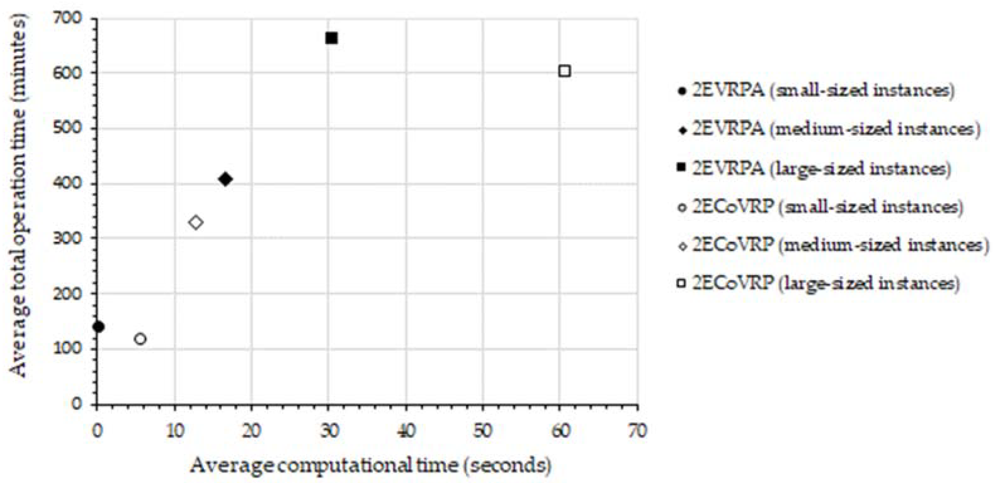
Figure 4 shows the comparative analysis for the two models, i.e., the 2EVRPA and the 2ECoVRP, and the solution methods, i.e., exact algorithm and tabu search algorithm. It is observed that the 2ECoVRP approach performs better than 2EVRPA for all scales of instances. It is important to note that a trade-off, however, exists between the achieved the best solution, i.e., the average total operation time, and the average computational time. To achieve lower total operation time, it generally requires longer computational time. An exception is, however, observed for medium-size instances in which the computational time for the best total operation time can be achieved with a shorter computational time. The result is of course desirable, but it is important to note that the medium-size instances were generated using 19–28 nodes out of 49 nodes, so the results are highly influenced by the selected node configurations. Detail analysis was further conducted to measure the standard deviation of the best solution for the 2ECoVRP approach. It was found that the standard deviation for medium-size instances was higher, at 126 min, than that of small-size instances. at 26 min, and that of large-size instances, at 33 min, indicating a wider variance of total operation time for medium-size instances.
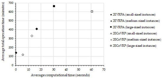
Figure 4.
Comparative analysis between the 2EVRPA and the 2ECoVRP.
With respect to the solution method, it seems that the tabu search algorithm is acceptable because it performs almost as well as the exact algorithm, as indicated by a slight difference when compared to the exact algorithm in the small-size instances. Because the tabu search algorithm has been able to solve the medium-size and large-size instances with a good-quality solution in sensible computational time, the tabu search is therefore suggested to be used as the solution method for the 2ECoVRP model.
4.4. Sensitivity Analysis
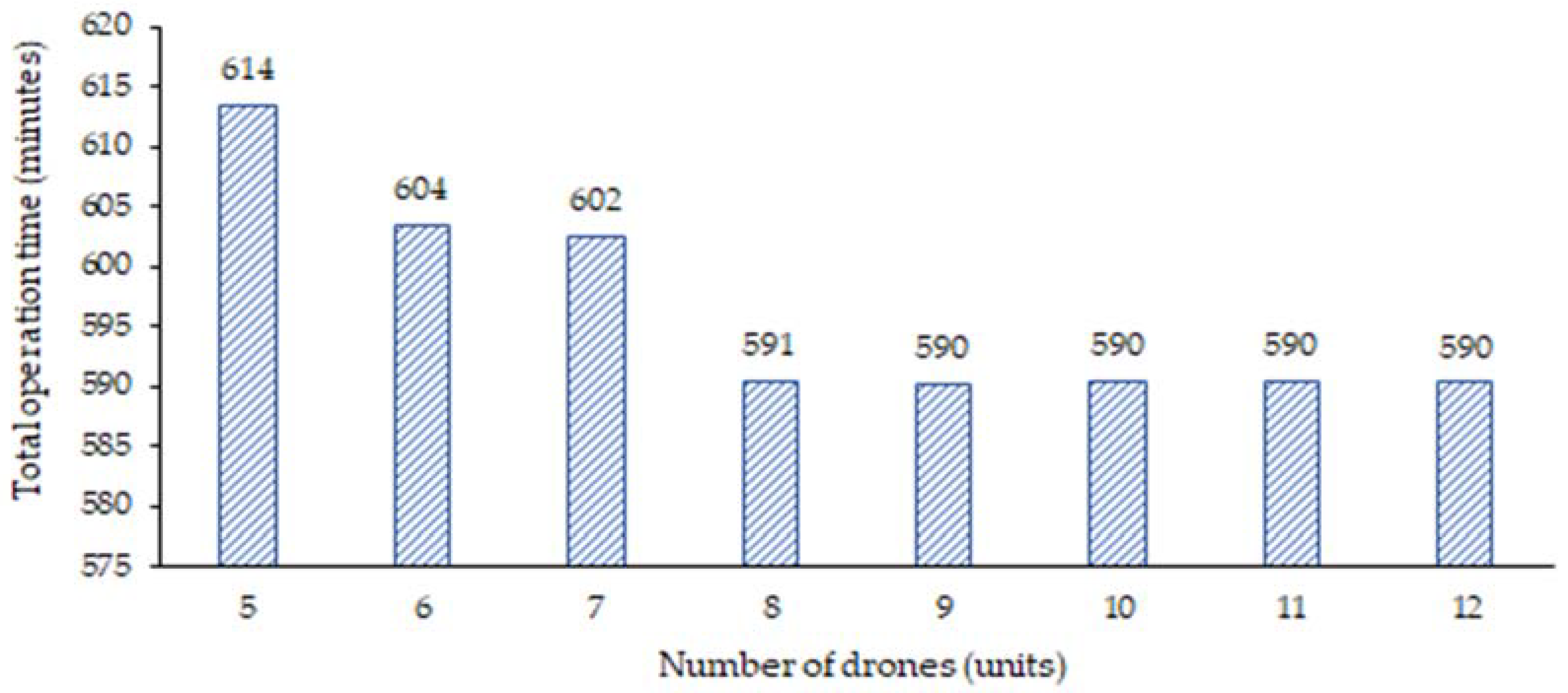
Sensitivity analysis is conducted to analyze the sensitivity of the total operation time due to changes in the number of drones. Figure 5 demonstrates that a lower number of drones corresponds to a higher total operation time of post-disaster assessment. In contrast, the more drones, the faster the assessment operation of post-disaster assessment. For instance, the addition of three drones, from five drones to eight drones, results in a shorter operation time of 23 min. Nevertheless, it is important to note that more drones are not always coupled with the faster operation. It appears that additional drones after the deployment of eight drones do not lead to a significant reduction of the total operation time. It can be argued that the operation time of post-disaster assessment is also constrained by the given network configuration, particularly the number and location of stopover points as shown in Figure 2, the total areas to be mapped, and the assumption that each motorcycle can only be mounted by one drone.

Figure 5.
Sensitivity analysis considering changes in the number of drones.
4.5. The Effect of Drone Configuration on the Operation Time
In addition to network configuration as previously discussed, the operation of hybrid aerial and ground vehicles is also influenced by drone configuration. This subsection, therefore, evaluates the effect of various drone configurations on the total operation time. Table 7 presents four drone configurations concerning flight altitude and battery capacity because these two parameters are considered to be influential factors in drone operation. The drone operated at a higher flight altitude has a higher capability to capture wider areas; however, the flight time is lower than that when operated at a lower altitude due to faster depletion of battery capacity. Similarly, the drone with a bigger battery capacity has a longer flight time. The large-size instances were used for the analysis.
Table 7.
Drone configurations.
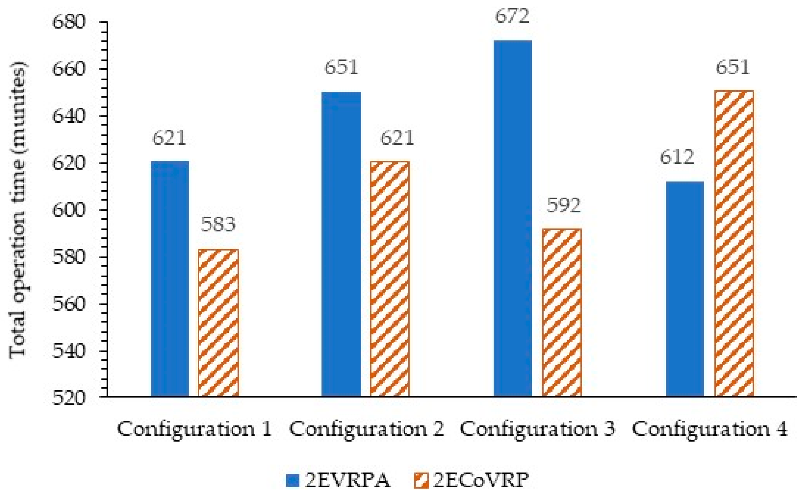
Figure 6 demonstrates that the 2ECoVRP performs better than 2EVRPA in all drone configuration settings, as indicated by the lower operation time. It is not surprising because the previous findings have demonstrated the superiority of the 2ECoVRP model. It can be argued that multi-visits in the 2ECoVRP helps to reduce the operation time significantly.

Figure 6.
Performance comparison of various drone configurations for the selected large-size instances.
The results indicate that the best drone configuration is when the drone with a battery capacity of 120 min and is operated at a flight altitude of 70 m. It is worth noting that when the battery capacity of the drone is reduced by 20 min, the total operation time is longer by 8.65 min and 51.5 min for 2ECoVRP and 2EVRPA, respectively (see Configuration 3). Similarly, when the flight altitude was set at about twice as high, the operation took an additional time of 28.88 min for 2ECoVRP and a lower time by 21.73 min for 2EVRPA (see Configuration 2). When comparing the result of Configuration 2 with that of Configuration 4, it was found that the reduction of battery capacity by 10 min results in a longer operation time of 29.77 min for 2ECoVRP and a lower operation time by 38.2 min for 2EVRPA. It appears that some inconclusive results were found for the effect of the flight altitude on the operation time and the effect of battery capacity on the operation time for the EVRPA.
Further investigation was conducted to explore the effect of a single operation parameter, i.e., battery capacity, on the best operation time. The investigation was based on Configuration 1 as the best configuration, which was modified by varying its battery capacities. Given the flight altitude of 70 m, Figure 7 indicates that higher battery capacity results in faster operation time. In contrast, using a lower battery capacity results in a significantly longer operation time. The improvement of the total operation time, however, does not seem to be linear. The increased battery capacity of more than 110 min does not lead to a significant reduction of the operation time. This implies that it is important to find the optimal battery capacity that fits a given post-disaster assessment operation so that the assessment operation is efficient.
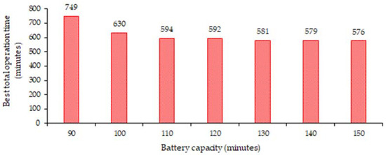
Figure 7.
The effect of battery capacity on operation time.
The aforementioned findings indicate that both flight altitude and battery capacity also contribute to the efficient assessment operation. It implies that further study exploring the optimal setting of drone operation for flight altitude and battery capacity is required.
4.6. Practical Implications
Although sustainability is not a new concept, its implementation within humanitarian operations has only recently been realized. A sustainable system generally rests on the continuous awareness that the objectives of sustainability, i.e., economic (e.g., cost), social (e.g., fairness), and ecological (e.g., emissions) goals are met. Therefore, the present study suggests that planning for post-disaster assessment such as the implementation of the hybrid aerial and ground vehicle system should be conducted not only to facilitate more quick and accurate assessment efficiently but also to reduce resources used.
Concerning the ecological goal, the deployment of the technology, i.e., the drone, for post-disaster assessment helps to reduce fuel consumption, consequently less GHG emissions and lower cost. Studies on life-cycle assessment for drones by Figliozzi [11] and Koiwanit [12] have indicated that drone is one of the most environmentally friendly transportation options. However, the deployment of the drone should also be accompanied by the efficient operation of the drone. The results imply that the efficiency of the hybrid aerial and ground vehicle operation depends on the network configuration, the routings of both vehicles, and the operation parameters such as flight altitude and battery capacity of the drone. To facilitate efficient routing of both the ground vehicle and the drone, the results imply that the 2ECoVRP approach solved by the tabu search algorithm seems to be promising as it only requires one minute to obtain the optimum routings of both vehicles. The findings also imply that operation settings should be explored further for a more efficient operation. For the studied case, it is suggested to deploy a maximum of eight drones with a flight altitude of 70 m and battery capacity of 120 min. The findings can be used by the search and rescue team of the Regional Disaster Agency to improve the efficiency and effectiveness of the post-disaster assessment.
Concerning the social aspect, the hybrid aerial and ground vehicle system allows accessing wider areas, as the drone can access areas that are inaccessible by the ground vehicle, thus facilitating fairness for the remote areas. Hence, the deployment of the hybrid aerial and ground vehicle at its optimal operation not only provides immediate and accurate assessment, which is crucial for emergency response operation, but also facilitates the sustainability aspect of the operations in terms of environmental, economic, and social goals.
5. Conclusions and Future Research
Due to its critical role of post-disaster assessment toward timely and effective response, an innovative and efficient approach to carry out the assessment is required. The present study proposes and evaluates the Two-Echelon Vehicle Routing Problem combined with Assignment (2EVRPA) and Two-Echelon Collaborative Vehicle Routing Problem (2ECoVRP) to evaluate optimal routings of both aerial and ground vehicles, which gives the minimum operation time for post-disaster assessment. The developed models were applied to solve the post-disaster assessment for the Mount Merapi eruption in Yogyakarta, Indonesia, to demonstrate its applicability to a real problem. A set of numerical experiments based on the empirical case were conducted. Both the exact algorithm and the tabu search algorithm were implemented to solve both models.
The findings indicate that the 2ECoVRP performs better than 2EVRPA in terms of the total operation time. It can be argued that the 2ECoVRP facilitates the more efficient operation of the drone by allowing multiple visits in one go. The average operation time to assess all mapping points is about 10 h, which is relatively faster than the current practice. Hence, the 2ECoVRP seems to be a promising approach to evaluate the routing of the hybrid aerial-ground vehicle system for post-disaster assessment. It is worth noting that a trade-off exists between the best solution and computational time. The computational time of the 2ECoVRP is about twice as long as that of the 2EVRPA for large instances. However, as the computational time for the 2ECoVRP is about one minute for large instances, it is considered reasonable and practical. It is also important to note that the tabu search algorithm can obtain optimal solutions that are comparable to those of exact algorithms, i.e., branch and bound as well as branch and cut methods, in a reasonable time. It is therefore suggested to be deployed to solve the 2ECoVRP.
Despite its contribution, some limitations of the present study need to be highlighted. First, the study has not compared the performance of the tabu search algorithm with other heuristics methods. The exploration for a more effective and efficient method to solve for the 2ECoVRP is therefore suggested as a potential avenue for future research. Second, the study has limited numerical analysis for different operational parameters such as flight altitude, drone specifications (e.g., battery capacity, mapping rate, speed), and the network configuration. However, the findings imply that the drone configuration settings (i.e., flight altitude and the drone’s battery capacity) influence the total operation time. Future studies could therefore extend the present study to explore the best solution by considering both network configuration and drone configuration. Last but not least, the present study deals with the deterministic problem. Due to high uncertainty corresponding to humanitarian operations, it is, therefore, necessary to evaluate the effectiveness of the obtained best solution in a dynamic environment setting. A hybrid optimization-simulation method such as that developed by Sopha, et al., [48] is thus suggested for other potential future research to test the effectiveness of the solution to support more effective and efficient post-disaster assessment practices.
Author Contributions
Conceptualization, B.M.S. and A.A.N.P.R.; methodology, A.A.N.P.R., B.M.S. and R.I.L.; software, A.A.N.P.R. and R.I.L.; validation, A.A.N.P.R., B.M.S. and R.I.L.; formal analysis, B.M.S. and A.A.N.P.R.; investigation, B.M.S., A.A.N.P.R., R.I.L. and A.M.S.A.; resources, B.M.S.; data curation, B.M.S. and A.M.S.A.; writing—original draft preparation, B.M.S. and A.A.N.P.R.; writing—review and editing, B.M.S., A.A.N.P.R. and A.M.S.A.; visualization, R.I.L.; project administration, B.M.S.; funding acquisition, B.M.S. All authors have read and agreed to the published version of the manuscript.
Funding
This research is funded by the Indonesian Ministry of Education, Culture, Research and Technology through World-Class Research (WCR) Scheme managed by Universitas Gadjah Mada (Contract No. 4497/UN1/DITLIT/DIT-LIT/PT/2021).
Institutional Review Board Statement
Not applicable.
Informed Consent Statement
Not applicable.
Data Availability Statement
The study did not report any data.
Acknowledgments
The authors would also like to thank the editor and anonymous referees for their valuable comments and suggested improvements.
Conflicts of Interest
The authors declare no conflict of interest.
Appendix A
Table A1.
Depots, stopover points, and target/mapping points.
Table A1.
Depots, stopover points, and target/mapping points.
| Symbol | Name | Latitude | Longitude | Area (m2) | Symbol | Name | Latitude | Longitude | Area (m2) |
|---|---|---|---|---|---|---|---|---|---|
| 1 | Depot 1 | −7.6575 | 110.443611 | 30 | Mapping Point 21 | −7.614167 | 110.453611 | 331,191 | |
| 2 | Depot 2 | −7.649167 | 110.443611 | 31 | Mapping Point 22 | −7.622222 | 110.455277 | 243,969 | |
| 3 | Depot 3 | −7.638889 | 110.445277 | 32 | Mapping Point 23 | −7.629444 | 110.455833 | 175,076 | |
| 4 | Depot 4 | −7.639444 | 110.425555 | 33 | Mapping Point 24 | −7.65 | 110.459444 | 150,000 | |
| 5 | Depot 5 | −7.691389 | 110.475833 | 34 | Mapping Point 25 | −7.651667 | 110.455555 | 131,500 | |
| 6 | Depot 6 | −7.648889 | 110.391944 | 35 | Mapping Point 26 | −7.639444 | 110.448333 | 169,500 | |
| 7 | Depot 7 | −7.659444 | 110.470277 | 36 | Mapping Point 27 | −7.636111 | 110.449166 | 120,000 | |
| 8 | Depot 8 | −7.668056 | 110.472777 | 37 | Mapping Point 28 | −7.635511 | 110.457391 | 140,750 | |
| 9 | Depot 9 | −7.648056 | 110.468333 | 38 | Mapping Point 29 | −7.590556 | 110.442222 | 227,563 | |
| 10 | Mapping Point 1 | −7.639444 | 110.462777 | 244,696 | 39 | Mapping Point 30 | −7.574185 | 110.443737 | 77,500 |
| 11 | Mapping Point 2 | −7.628889 | 110.464722 | 174,139 | 40 | Mapping Point 31 | −7.596667 | 110.442777 | 185,925 |
| 12 | Mapping Point 3 | −7.631111 | 110.466111 | 196,657 | 41 | Stopover Point 1 | −7.6665221 | 110.4714306 | |
| 13 | Mapping Point 4 | −7.626111 | 110.464166 | 141,113 | 42 | Stopover Point 2 | −7.6739458 | 110.464487 | |
| 14 | Mapping Point 5 | −7.621667 | 110.462222 | 229,684 | 43 | Stopover Point 3 | −7.6587427 | 110.4558261 | |
| 15 | Mapping Point 6 | −7.5975 | 110.459444 | 125,100 | 44 | Stopover Point 4 | −7.6384602 | 110.4593284 | |
| 16 | Mapping Point 7 | −7.584722 | 110.457222 | 139,612 | 45 | Stopover Point 5 | −7.6316921 | 110.4569936 | |
| 17 | Mapping Point 8 | −7.574167 | 110.454722 | 240,192 | 46 | Stopover Point 6 | −7.6205943 | 110.4545169 | |
| 18 | Mapping Point 9 | −7.677222 | 110.461666 | 93,110 | 47 | Stopover Point 7 | −7.6028011 | 110.4496507 | |
| 19 | Mapping Point 10 | −7.674722 | 110.463333 | 99,968 | 48 | Stopover Point 8 | −7.5893084 | 110.4629461 | |
| 20 | Mapping Point 11 | −7.671944 | 110.463055 | 80,450 | 49 | Stopover Point 9 | −7.5877972 | 110.4485526 | |
| 21 | Mapping Point 12 | −7.669722 | 110.4625 | 117,905 | 40 | ||||
| 22 | Mapping Point 13 | −7.662778 | 110.457777 | 133,995 | 41 | ||||
| 23 | Mapping Point 14 | −7.657778 | 110.4575 | 66,734 | 42 | ||||
| 24 | Mapping Point 15 | −7.662778 | 110.466111 | 111,311 | 43 | ||||
| 25 | Mapping Point 16 | −7.669167 | 110.471666 | 77,284 | 44 | ||||
| 26 | Mapping Point 17 | −7.582778 | 110.451111 | 331,191 | 45 | ||||
| 27 | Mapping Point 18 | −7.595556 | 110.451111 | 253,449 | 46 | ||||
| 28 | Mapping Point 19 | −7.596667 | 110.448333 | 232,592 | 47 | ||||
| 29 | Mapping Point 20 | −7.610556 | 110.450555 | 291,372 | 48 |
References
- Kovacs, G.; Spens, K.M. Identifying Challenges in Humanitarian Logistics. Int. J. Phys. Dist. Log. Manag. 2009, 39, 506–528. [Google Scholar] [CrossRef]
- Hassanalian, M.; Abdelkefi, A. Classifications, Applications, and Design Challenges of Drones: A Review. Prog. Aerosp. Sci. 2017, 91, 99–131. [Google Scholar] [CrossRef]
- Viloria, D.R.; Solano-Charris, E.L.; Muñoz-Villamizar, A.; Montoya-Torres, J.R. Unmanned Aerial Vehicles/Drones in Vehicle Routing Problems: A Literature Review. Int. Trans. Oper. Res. 2021, 28, 1626–1657. [Google Scholar] [CrossRef]
- Mishra, B.; Garg, D.; Narang, P.; Mishra, V. Drone-Surveillance for Search and Rescue in Natural Disaster. Comp. Comms. 2020, 156, 1–10. [Google Scholar] [CrossRef]
- Sopha, B.M.; Doni, R.E.; Asih, A.M.S. Mount Merapi Eruption: Simulating Dynamic Evacuation and Volunteer Coordination using Agent-Based Modeling Approach. J. Humanit. Logist. Supply Chain Manag. 2019, 9, 292–322. [Google Scholar] [CrossRef]
- McRae, J.N.; Gay, C.J.; Nielsen, B.M.; Hunt, A.P. Using an Unmanned Aircraft System (Drone) to Conduct a Complex High Altitude Search and Rescue Operation: A Case Study. Wilderness Environ. Med. 2019, 30, 287–290. [Google Scholar] [CrossRef] [Green Version]
- Shavarani, S.M. Multi-Level Facility Location-Allocation Problem for Post-Disaster Humanitarian Relief Distribution. J. Humanit. Logist. Supply Chain Manag. 2019, 9, 70–81. [Google Scholar] [CrossRef]
- Tatham, P.; Stadler, F.; Murray, A.; Shaban, R.Z. Flying Maggots: A Smart Logistic Solution to an Enduring Medical Challenge. J. Humanit. Logist. Supply Chain Manag. 2017, 7, 172–193. [Google Scholar] [CrossRef]
- Peckham, R.; Sinha, R. Anarchitectures of Health: Futures for the Biomedical Drone. Glob. Public Health 2019, 14, 1204–1219. [Google Scholar] [CrossRef]
- Poljak, M.; Šterbenc, A. Use of Drones in Clinical Microbiology and Infectious Diseases: Current Status, Challenges and Barriers. Clin. Microbiol. Infect. 2010, 26, 425–430. [Google Scholar] [CrossRef]
- Figliozzi, M.A. Lifecycle Modeling and Assessment of Unmanned Aerial Vehicles (Drones) CO2e Emissions. Transp. Res. Part D Transp. Environ. 2017, 57, 251–261. [Google Scholar] [CrossRef]
- Koiwanit, J. Analysis of Environmental Impacts of Drone Delivery on an Online Shopping System. Adv. Clim Chang. Res. 2018, 9, 201–207. [Google Scholar] [CrossRef]
- Sopha, B.M.; Triasari, A.I.; Cheah, L. Sustainable Humanitarian Operations: Multi-Method Simulation for Large-Scale Evacuation. Sustainability 2021, 13, 7488. [Google Scholar] [CrossRef]
- Erdelj, M.; Król, M.; Natalizio, E. Wireless Sensor Networks and Multi-UAV Systems for Natural Disaster Management. Comput. Netw. 2017, 124, 72–86. [Google Scholar] [CrossRef]
- Estrada, M.A.R.; Ndoma, A. The Uses of Unmanned Aerial Vehicles –UAV’s- (Or Drones) in Social Logistics: Natural Disasters Response and Humanitarian Relief Aid. Procedia Comput. Sci. 2019, 149, 375–383. [Google Scholar] [CrossRef]
- Moshref-Javadi, M.; Lee, S.; Winkenbach, M. Design and Evaluation of a Multi-Trip Delivery Model with Truck and Drones. Transp. Res. Part E Logist. Transp. Rev. 2020, 136, 101887. [Google Scholar] [CrossRef]
- Jeong, H.Y.; Song, B.D.; Lee, S. Truck-Drone Hybrid Delivery Routing: Payload-Energy Dependency and No-Fly Zones. Int. J. Prod. Econ. 2019, 214, 220–233. [Google Scholar] [CrossRef]
- Crişan, G.C.; Nechita, E. On a Cooperative Truck-And-Drone Delivery System. Procedia Comput. Sci. 2019, 159, 38–47. [Google Scholar] [CrossRef]
- Chowdhury, S.; Emelogu, A.; Marufuzzaman, M.; Nurre, S.G.; Bian, L. Drones for Disaster Response and Relief Operations: A Continuous Approximation Model. Int. J. Prod. Econ. 2017, 188, 167–184. [Google Scholar] [CrossRef]
- Cannioto, M.; D’Alessandro, A.; Bosco, G.L.; Scudero, S.; Vitale, G. Brief Communication: Vehicle Routing Problem and UAV Application in the Post-Earthquake Scenario. Nat. Hazards Earth Syst. Sci. 2017, 17, 1939–1946. [Google Scholar] [CrossRef] [Green Version]
- Oruc, B.E.; Kara, B.Y. Post-Disaster Assessment Routing Problem. Transp. Res. Part B Methodol. 2018, 116, 76–102. [Google Scholar] [CrossRef]
- Luo, Z.; Liu, Z.; Shi, J.A. Two-Echelon Cooperated Routing Problem for a Ground Vehicle and Its Carried Unmanned Aerial Vehicle. Sensors 2017, 17, 1144. [Google Scholar] [CrossRef] [PubMed] [Green Version]
- Otto, A.; Agatz, N.; Campbell, J.; Golden, B.; Pesch, E. Optimization Approaches for Civil Applications of Unmanned Aerial Vehicles (Uavs) or Aerial Drones: A Survey. Networks 2018, 72, 411–458. [Google Scholar] [CrossRef]
- Asih, A.M.S.; Sopha, B.M.; Kriptaniadewa, G. Comparison Study of Metaheuristics: Empirical Application of Delivery Problems. Int. J. Eng. Bus. Manag. 2017, 9, 1–12. [Google Scholar] [CrossRef]
- Streitfeld, D. Amazon Delivers Some Pie in the Sky. The New York Times, 3 November 2013; 1. [Google Scholar]
- Khoufi, I.; Laouiti, A.; Adjih, C. A Survey of Recent Extended Variants of the Traveling Salesman and Vehicle Routing Problems for Unmanned Aerial Vehicles. Drones 2019, 3, 66. [Google Scholar] [CrossRef] [Green Version]
- Kellerman, R.; Biehle, T.; Fischer, L. Drones for Parcel and Passenger Transportation: A Literature Review. Transp. Res. Interdiscip. Perspect. 2020, 4, 100088. [Google Scholar] [CrossRef]
- Bruni, M.E.; Khodaparasti, S.; Beraldi, P. The Selective Minimum Latency Problem under Travel Time Variability: An Application to Post-Disaster Assessment Operations. Omega 2020, 92, 102154. [Google Scholar] [CrossRef]
- Wang, X.; Poikonen, S.; Golden, B. The Vehicle Routing Problem with Drones: Several Worst-Case Results. Optim. Lett. 2016, 11, 679–697. [Google Scholar] [CrossRef]
- Murray, C.C.; Chu, A.G. The Flying Sidekick Traveling Salesman Problem: Optimization of Drone-Assisted Parcel Delivery. Transp. Res. Part C Emerg. Technol. 2015, 54, 86–109. [Google Scholar] [CrossRef]
- Agatz, N.; Bouman, P.; Schmidt, M. Optimization Approaches for the Traveling Salesman Problem with Drone. Transp. Sci. 2016, 52, 965–981. [Google Scholar] [CrossRef]
- Tu, P.A.; Dat, N.T.; Dung, P.Q. Traveling Salesman Problem with Multiple Drones. In SoICT 2018, Proceedings of the Ninth International Symposium on Information and Communication Technology, Danang City, Vietnam, 6–7 December 2018; ACM: New York, NY, USA, 2018; pp. 46–53. [Google Scholar]
- Kitjacharoenchai, P.; Ventresca, M.; Moshref-Javadi, M.; Lee, S.; Tanchoco, J.M.; Brunese, P.A. Multiple Traveling Salesman Problem with Drones: Mathematical Model and Heuristic Approach. Comput. Ind. Eng. 2019, 129, 14–30. [Google Scholar] [CrossRef]
- Luo, Z.; Poon, M.; Zhang, Z.; Liu, Z.; Lim, A. The Multi-visit Traveling Salesman Problem with Multi-Drones. Transp. Res. Part C Emerg. Technol. 2021, 128, 103172. [Google Scholar] [CrossRef]
- Poikonen, S.; Wang, X.; Golden, B. The Vehicle Routing Problem with Drones: Extended Models and Connections. Networks 2017, 70, 34–43. [Google Scholar] [CrossRef]
- Coelho, B.N.; Coelho, V.N.; Coelho, I.M.; Ochi, L.S.; Haghnazar, K.R.; Zuidema, D.; Lima, M.S.; da Costa, A.R. A Mul-ti-objective Green UAV Routing Problem. Comput. Oper. Res. 2017, 88, 306–315. [Google Scholar] [CrossRef]
- Cheng, C.; Adulyasak, Y.; Rousseau, L.M. Formulations and Exact Algorithms for Drone Routing Problem; Centre Interuniversitaire de Recherche sur les Reseaux D’entreprise, la Logistique et le Transpor: Montreal, QC, Canada, 2018. [Google Scholar]
- Cuda, R.; Guastaroba, G.; Speranza, M.G. A Survey on Two-Echelon Routing Problems. Comput. Oper. Res. 2015, 55, 185–199. [Google Scholar] [CrossRef]
- Perboli, G.; Tadei, R.; Vigo, D. The Two-Echelon Capacitated Vehicle Routing Problem: Models and Math-Based Heuristics. Transp. Sci. 2011, 45, 364–380. [Google Scholar] [CrossRef] [Green Version]
- Redi, A.A.N.P.; Jewpanya, P.; Kurniawan, A.C.; Persada, S.F.; Nadlifatin, R.; Dewi, O.A.C. A Simulated Annealing Algorithm for Solving Two-Echelon Vehicle Routing Problem with Locker Facilities. Algorithms 2020, 13, 218. [Google Scholar] [CrossRef]
- Glover, F.; Laguna, M. Tabu Search. In Handbook of Combinatorial Optimization; Du, D.Z., Pardalos, P.M., Eds.; Springer: Boston, MA, USA, 1998. [Google Scholar] [CrossRef]
- Semet, F.; Taillard, E. Solving Real-Life Vehicle Routing Problems Efficiently Using Tabu Search. Ann. Oper. Res. 1993, 41, 469–488. [Google Scholar] [CrossRef]
- Chao, I.-M. A Tabu Search Method for the Truck and Trailer Routing Problem. Comput. Oper. Res. 2002, 29, 33–51. [Google Scholar] [CrossRef]
- Scheuerer, S. A Tabu Search Heuristic for the Truck and Trailer Routing Problem. Comput. Oper. Res. 2006, 33, 894–909. [Google Scholar] [CrossRef]
- Boccia, M.; Crainic, T.G.; Sforza, A.; Sterle, C. A Metaheuristic for a Two-Echelon Location-Routing Problem. In Experimental Algorithms SEA 2010: Lecture Notes in Computer Science; Festa, P., Ed.; Springer: Berlin/Heidelberg, Germany, 2010; Volume 6049, pp. 288–301. [Google Scholar] [CrossRef]
- Venkatachalam, S.; Sundar, K.; Rathinam, S. A Two-Stage Approach for Routing Multiple Unmanned Aerial Vehicles with Stochastic Fuel Consumption. Sensors 2018, 18, 3756. [Google Scholar] [CrossRef] [PubMed] [Green Version]
- Liperda, R.I.; Pewira Redi, A.A.M.; Sekaringtyas, N.N.; Astiana, H.B.; Sopha, B.M.; Asih, A.M.S. Simulated Annealing Algorithm Performance on Two-Echelon Vehicle Routing Problem-Mapping Operation with Drones. In Proceedings of the IEEE International Conference on Industrial Engineering and Engineering Management, Singapore, 14–17 December 2020; IEEE: Piscataway, NJ, USA, 2020; pp. 1142–1146. [Google Scholar]
- Sopha, B.M.; Siagian, A.; Asih, A.M.S. Simulating Dynamic Vehicle Routing Problem using Agent-Based Modeling and Simulation. In Proceedings of the IEEE International Conference on Industrial Engineering and Engineering Management, Bali, Indonesia, 4–7 December 2016; IEEE: Piscataway, NJ, USA, 2016; pp. 1335–1339. [Google Scholar]


Publisher’s Note: MDPI stays neutral with regard to jurisdictional claims in published maps and institutional affiliations. |
© 2021 by the authors. Licensee MDPI, Basel, Switzerland. This article is an open access article distributed under the terms and conditions of the Creative Commons Attribution (CC BY) license (https://creativecommons.org/licenses/by/4.0/).