A Crash Injury Model Involving Autonomous Vehicle: Investigating of Crash and Disengagement Reports

Abstract

Autonomous vehicles (AVs) are being extensively tested on public roads in several states in the USA, such as California, Florida, Nevada, and Texas. AV utilization is expected to increase into the future, given rapid advancement and development in sensing and navigation technologies. This will eventually lead to a decline in human driving. AVs are generally believed to mitigate crash frequency, although the repercussion of AVs on crash severity is ambiguous. For the data-driven and transparent deployment of AVs in California, the California Department of Motor Vehicles (CA DMV) commissioned AV manufacturers to draft and publish reports on disengagements and crashes. This study performed a comprehensive assessment of CA DMV data from 2014 to 2019 from a safety standpoint, and some trends were discerned. The results show that decrement in automated disengagements does not necessarily imply an improvement in AV technology. Contributing factors to the crash severity of an AV are not clearly defined. To further understand crash severity in AVs, the features and issues with data are identified and discussed using different machine learning techniques. The CA DMV accident report data were utilized to develop a variety of crash AV severity models focusing on the injury for all crash typologies. Performance metrics were discussed, and the bagging classifier model exhibited the best performance among different candidate models. Additionally, the study identified potential issues with the CA DMV data reporting protocol, which is imperative to share with the research community. Recommendations are provided to enhance the existing reports and append new domains.

1. Introduction

Autonomous vehicles (AVs) have the potential to revolutionize the transport industry by alleviating congestion, improving safety, and reducing accidents. Consequently, the transport industry will benefit from AV deployment, but the impacts on the auxiliary industries are debatable. As AV manufacturing companies move from research to prototype to production, the generation of data increases exponentially. This data lake (conditional to availability) could elucidate the ambiguity around crash risk.

The ability of AVs to mitigate crash risk caused by human error has raised the expectation of a downtrend in conventional critical safety events. However, the inclusion of AVs within the system can result in new safety challenges associated with poorly maintained road markings and light reflections affecting the vehicle sensors. AV communication faults, cybersecurity, and disengagements also influence crash prevalence [1]. Furthermore, it is essential to note that there is even less understanding about the influence these and other AV features have on crash severity.

The estimation of the economic and social burden caused by road traffic crashes involving AVs requires a thorough understanding of the factors affecting the crash frequency or, given that a crash has occurred, the attributes that can alleviate or aggravate the cost and injury in the crash. Although AV trials generate a vast amount of data, these data cannot be acquired because of data privacy: especially when personal information is involved. Furthermore, synthetic data created by traffic microsimulation models (e.g., [2,3]) and surrogate safety assessment models cannot represent the new or unprecedented crash sources present in AVs. As a result, these models are advantageous but not necessarily an exact representation of the AV scenario. For the safe and transparent deployment of AVs in California, the California Department of Motor Vehicles (CA DMV) commissioned AV manufacturers to draft and publish two reports: a disengagement report and a crash report. A disengagement report is a summary of events where the software (“brain”) of a car disengages automatically (automated) or the disengagement is initiated by the human driver (manual). A crash report is a detailed rundown of events that resulted in a collision and/or damage to property and injuries. These reports are filed by manufacturers conforming to guidelines given by the CA DMV. Whilst there are few implicit fields and fewer data points than typical crash datasets in the literature, it is the best accessible dataset because of open-source availability. Additionally, these data represent the real-world scenario since they comprehend the unprecedented crash causes, unlike microsimulation models. For these reasons, we used CA DMV data, which have been used in a few recent studies [4,5,6,7,8,9,10,11,12,13,14].

This paper provides a detailed review of critical issues associated with crash severity and develops a model for crash severity of AVs. Consequently, the model performance is presented. Furthermore, a detailed review of the limitations of reporting protocol is discussed. Additionally, a comprehensive analysis of the DMV crash data and disengagement data is performed, and expansion on previous studies’ conclusions is presented. This study will aid AV manufacturers and actuarial organizations to evaluate the risks and associated burden in an AV crash. Necessarily, this study also assists the policymakers in updating the present reporting system. The following sections provide a literature review, study area and data description, data analysis and crash model formulation, discussion, limitations, and extension.

2. Literature Review

Before detailing the data and modelling exercise, it is essential to acknowledge recent relevant literature concerning the focal topics of the research. The following Section 2.1 and Section 2.2 present a background to the development of crash severity models in the AV landscape and the application of CA DMV data by other researchers.

2.1. Existing Crash Severity Models and Their Limitations in AV Deployed Scenario

Since the number and severity of crashes affect overall road safety, numerous studies have investigated these measures. Existing crash severity models have been developed for different combinations of dependent (outcome) and independent (explanatory) variables. These studies can be clustered into three significant brackets: transport viewpoint, crash analysis viewpoint, and medical viewpoint [15].

The transport viewpoint studies concentrated on transport-related explanatory variables, e.g., traffic (speed, flow, and density), road, and weather characteristics [16,17,18,19]. Some of these characteristics are expected to alter with AV penetration, and existing severity models need alteration. For instance, AVs are expected to manoeuver efficiently in platoons with decreased headways resulting in different network throughput, compared to the present scenario [20,21]. In addition, AVs’ negligible or absent reaction time stipulates to revise roadway design manuals [4], e.g., implementation of taut turning radii because of negligible minimum sight distances of AVs [21]. Additionally, road maintenance (e.g., repainting markings) could reduce the disengagements [6], affecting crash frequency and severity. In CA DMV reports, Waymo and Mercedes specifically reported the weather as a disengagement cause, indicating the pivotal association of weather and AV performance.

The second category is the crash analysis [22,23,24] viewpoint, which focused on vehicle characteristics such as vehicle’s mass, size, age, and facilities [25] and impact characteristics such as impact speed, collision type, and angle of crash. Increase in manual/conventional vehicle age is found to elevate crash severity [26]. It is speculative that AV hardware’s age should elevate crash severity; however, the age of software (AV “brain”) should alleviate crash severity since AV brains have more training data and have been exposed to a greater variety of hazards. Additionally, an old study [27] evaluated the severity and frequency of rear-end crashes for automated and human driver highway systems. They concluded that automated systems are anticipated to collide at less than 30% of the velocity of the human driver system. In addition, AV technology is competent in preventing all other collision typologies except rear-end crashes [5]. These studies exhibit a change in crash dynamics in the AV deployed environment, which stipulates the necessity of AV-focused crash severity models.

The third category of researchers approached severity from a medical point of view. A severity level (dependent variable) was quantified using the Abbreviated Injury Scale and Injury Severity Score [26,28,29,30]. The exploratory variables encompassed are human behaviour, demographics, and safety facility usage. Existing medical studies fail to incorporate a few issues, for instance, the “driver in the loop” concern in AVs. Automation could make tasks more difficult by removing the easy parts of a task [31]. The out-of-loop performance problems are a salient issue that has been widely documented as a potential negative consequence of automation [32]. Drivers’ increasing trust in AV systems becomes disconcerting on the grounds of “driver in loop” concern [4], and thus new studies examining this concern are vital.

2.2. Previous Studies Employing CA DMV Data

CA DMV data are the best open-source data available for external validation. Our study attempted to use the crash data involving AVs to investigate the safety impact of AVs on the transport system. To date, CA DMV data have been predominantly examined for trends in disengagements, crashes, human trust and reaction time [4], crash frequencies, dynamics, and damage analysis using crash reports [5], triggers and contributory factors of disengagements [6], potential causal relationships between the crashes and disengagements [9], and reliability of AVs by assessing the failures across a wide range of AV manufacturers [8]. Table 1 provides a summary of past research utilizing CA DMV data, including significant findings and insights.

Table 1. Summary of past studies employing CA DMV data.

Study	Significant Findings/Insights
Dixit et al. (2016)	The number of accidents observed has a significantly high correlation with the autonomous miles travelled. Differences were observed in reaction times based on the autonomous miles covered, disengagement type, and type of roadway. With an increase in the vehicle miles travelled, the reaction times were increased, which proposes an increased level of trust with more vehicle miles travelled. This is coined as the “trust effect”.
Favarò et al. (2017)	Did not support the argument that the prototype (anthropomorphic design) may be any “safer” (having a lower accident frequency) than the other make currently tested by Google. Sixty-two percent of autonomous vehicle accidents are rear-ended type. The number of accidents observed is strongly correlated with the autonomous miles travelled. Put forward the idea that plateau region of cumulative accident trend as a function of cumulative miles will signify that the AV technology is improving and getting close to “accident-free”.
Favarò et al. (2018)	Google Inc. adopted a distinction between two disengagement modes: failure detection and safety operations. The two categories can be tied back to the distinction between manual and automated initiation. The proposed wording dissociates the cause of the disengagement (failure detection and/or safety operations) from the actual modality of occurrence (manual vs. automated). The study stated that the definition provided by the DMV mixed these two. Proposed a distinction between exogenous and endogenous contributory factors of disengagements as an additional mandatory category that would need to be reported to the DMV. Exogenous/external factors are factors outside the control of the driver and/or manufacturer (e.g., weather, infrastructure condition, outside traffic), while endogenous/internal factors can be acted upon. The difference lies within the possible controllability of the factor.
Banerjee et al. (2018)	Drivers of AVs need to be equally vigilant as drivers of non-AV vehicles. With the widespread deployment of AVs, reaction-time-based accidents would become a recurrent failure mode due to the small size of the overall action window. Action window is the sum of detection time and reaction time. Sixty-four percent of disengagements were the result of issues in or inapt decisions made by the machine learning system. In terms of reliability per mission, AVs are 4.22 times worse than aeroplanes and 2.5 times better than surgical robots. These findings indicate that while individual modules of AV technology (e.g., control systems, vision systems) may have fully developed, entire AV systems are still in a “burn-in” phase.
Favarò et al. (2019)	“Trust effect” put forward by [4] was argued to be premature in the light of new data. Correlation between time to takeover and cumulative autonomous miles driven per month was statistically insignificant, indicating no improvement in trust with more experience. Correlation between the reported incidents per month and the mileage driven was analysed to investigate the “learning effect” of safety operation drivers, with seasoned drivers prone to negative correlation (considering that the Waymo fleet has higher miles than Mercedes-Benz).
Khattak et al. (2019)	Crash proportions between more recent and older tests were compared. Results display no statistically significant change in crash proportions over the two periods observed. Disengagements without crashes are more likely to be caused by factors related to other road participants.
Xu et al. (2019)	The property damage only (PDO) was taken as the reference level of the dependent variable. Bootstrap-based binary logistic regressions models were developed to investigate the factors contributing to the collision type and severity of AV-involved crashes. Significant variables contributing to the severity level of AV-involved crashes are driving mode, collision location, roadside parking, rear-end collision, and one-way road. Rear-end and sideswipe crashes account for 57.5% and 28.8% of total AV-involved crashes. Two vehicle movements were found to be a predominant occurrence that may lead to crash: (1) stopped AV and proceeding straight movement of conventional vehicle, (2) passing of following conventional vehicles over the ahead CAV vehicles.
Boggs et al. (2020)	Fixed and random parameters binary logistic regression models were developed for disengagement initiation. Location (highway or street), cause (environmental, another road user, hardware or software discrepancy, and planning discrepancy), and maturity of testing (month of testing) were found to be significant. The marginal effects of each explanatory variable were also illustrated. A random parameter model was found to be a better fit for the data. ADS testing maturity parameter emphasises that as the maturity of the testing increases by a month, the probability of a disengagement being initiated by ADS increases by 0.014. Unobserved heterogeneity is accounted for by encompassing the random parameter. The model underlines essential information that would cause inappropriate interpretations if the random parameter is not used. For example, the “trust” effect argued by (Dixit et al. 2016).
Wang et al. (2020)	Statistical analysis was applied for AV accidents on public roads, where over 3.7 million miles were tested by various manufacturers from 2014 to 2018. Results show that disengagement frequency varied from 2 × 10−4 to 3 disengagements per mile. Between 2014 and 2018, 63% of accidents were caused in autonomous mode, and roughly 6% were AVs, with 94% of accidents were by other parties. Most accidents are caused by other parties, and alerting and avoiding safety risks can improve safe decisions to prevent fatal accidents.
Das et al. (2020)	Bayesian latent class model identified six classes that correlated based on different variables and collision traits. Such variables included collision type, vehicle damage, operator injury severity, lighting conditions, number of vehicles involved, weather conditions, event prior to the collision, and if the vehicle was moving or stopped. Higher proportion of injury severity level was found to associate with turning, multi-vehicle collisions, sideswipe and rear-end collisions, and dark lighting conditions with streetlights. A higher likelihood of adverse weather-related accidents whilst the vehicle was in autonomous mode and stopped. The authors stated that there is a need for more advanced and robust collision narrative reporting to better assess collision likelihoods of autonomous vehicles.
Khattak et al. (2020)	Nested logit model was used with: (1) disengagement with a crash, (2) disengagement with no crash, and (3) no disengagement with a crash. Endogenous switching regime models were further used to find relationships of disengagements and crashes with consideration to endogeneity effects. Results found that factors relating to AV systems and other roadway participants increase the tendency of disengagement without a crash. Moreover, it was observed that disengagements lessen over time. Authors posited that disengagements are a part of AVs’ safe performance, and disengagement warnings should be used to avoid certain failures with current technology.

Building on the findings presented in Table 1, the novelty of our study was the investigation of the contributory and explanatory factors of AV damage crash severity and formulation of the AV crash damage severity model. Additionally, this study exhibited the dissonant implications of disengagement trends and proposed recommendations based on the rationales.

3. Study Area and Data Description

3.1. Study Area

CA DMV disengagement reports summarize failure events, categorized as autonomous disengagement or manual disengagement, albeit the distinction between these categories is implicit [6]. Our study used Google disengagement data because Google contributed 63.04% of total autonomous miles travelled (including 2019). Additionally, these data provide comprehensive details of disengagement events as compared with other manufacturers. On the other hand, the crash reports are a detailed description of the events that incurred property damage or injuries. From 2018, a new category of “vehicle damage description” has been appended in the crash reports. The vehicle damage description is perceived damage by the manufacturer’s authorized representative and hence not explicit. The data used in this study are the DMV disengagement and crash reports and Google traffic data. AV testing is permitted in San Francisco and San Jose cities in Silicon Valley, California, and the crash locations are mapped in Figure 1.

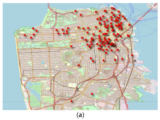
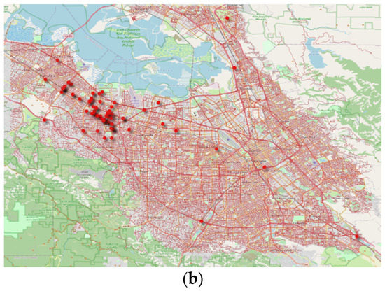
Figure 1. Crash locations superimposed on the street network: (a) San Francisco; (b) San Jose.

3.2. Data Description

A brief description of all the variables used in developing the AV damage severity model is presented in Table 2. Further, details of the data explicitly used during the modelling process are discussed in Section 4.3.1. A few important notes regarding the dataset are mentioned below.

Table 2. Descriptive statistics of variables.

Variable	Type	Definition	Descriptive Statistics
Vehicle number	Categorical	Number of vehicles involved	F(1) = 5%
			F(2) = 92%
			F(3) = 3%
Intersection	Categorical	= 1 if crash location was intersection; = 0 otherwise	F(0) = 37%
			F(1) = 63%
Signalized	Binary	= 1 with signals; = 0 without	F(0) = 51%
			F(1) = 49%
Parking provision	Binary	= 1 with parking provision; = 0 without or no information	F(1) = 56%
			F(0) = 44%
Mode	Binary	= 1 autonomous; = 0 conventional	F(1) = 54%
			F(0) = 46%
Fault	Binary	= 1 AV at fault; = 0 not at fault	F(1) = 12%
			F(0) = 88%
AV status	Binary	= 1 moving; = 0 stopped	F(1) = 57%
			F(0) = 43%
Other party’s vehicle status	Binary	= 1 moving; = 0 stopped	F(1) = 95%
			F(0) = 5%
Vehicle type	Categorical	= 1 two wheels (i.e., bicycle, scooter);	F(1) = 12%
		= 2 sub-compact/compact cars;	F(2) = 41%
		= 3 mid-size cars;	F(3) = 36%
		= 4 trucks/buses/trailers	F(4) = 12%
Collision type	Categorical	= 1 head-on;	F(1) = 6%
		= 2 sideswipe;	F(2) = 21%
		= 3 rear-end;	F(3) = 62%
		= 4 others	F(4) = 11%
Intersection type	Categorical	= 0 straight road	F(0) = 9%
		= 1 Y-intersection	F(1) = 11%
		= 2 T-intersection	F(2) = 15%
		= 3 Cross intersection	F(3) = 59%
		= 4 Complex intersection	F(4) = 5%

• The observed damage severity levels sustained by autonomous vehicles during the examination period have the following distribution: no damage (7.14%); minor damage (71.43%); moderate damage (20.41%); major damage (1.02%).
• The kinetic energy of a crash plays a crucial role in gauging crash severity [33,34]. The relative velocity of vehicles involved in the crash is missing for 176 out of 259 incidents.
• Vehicle type is the representation of vehicle size derived from the vehicle model stated in the reports. “Two wheels” type refers to vehicles with two wheels such as bikes, motorcycles, and scooters. Subcompact and compact cars are slightly smaller than mid-size cars with an inside volume between 2.4 m³ and 3.1 m³ by combining cargo and passenger volume. Mid-size vehicles are identified as possessing an interior volume of between 3.1 m³ and 3.4 m³. The last category is large vehicles, which represents trucks and buses in this study.

4. Data Analysis and Crash Model Formulation

CA DMV data from 14 October 2014 to 15 June 2020 were used for crash analysis and developing crash damage severity model. For disengagement analysis, we utilized CA DMV reports from 2014 to 2019 since disengagement reports were not available for 2020 at the time of this study. Testing was halted for a while due to the COVID-19 pandemic, and hence 2020 data were not considered for disengagement.

4.1. Crashes

The main concern regarding the adoption of AVs has been based on the grounds of safety. In this section, we perform an in-depth analysis, revisit some of the results, and expand on what was concluded in previous studies [4,5].

Figure 2 exhibits the distribution of crash typologies. Table 3 shows the distribution of crash typologies, driving mode, and party at fault. There were just two crash events where the AV was on autonomous mode and found to be at fault, highlighting the dearth of data related to at-fault AV crashes. In 88.42% (229/259) of all cases, the other party was found to be at fault. Within these cases, 52.90% (137/259) of the time the AV was found to be in autonomous mode. Of total crashes, 61.78% (160 out of 259) were rear-ended. Among these 160 rear-end cases, on 103 occasions, AV was on autonomous mode and not at fault. Rear-end crashes were the most prevalent (105 out of 160) of all the crashes when the AV was on autonomous mode. Authors posit that the dissonant and incompatible reaction time of AV and a human driver in a conventional car was the cause of several rear-end crashes. AVs are very efficient in avoiding collision with the leader (none or negligible reaction time involved). However, follower non-AV drivers cannot react efficiently and thus bump into the leader AV, which was postulated by [5]. Consequently, there is a need to revisit roadway design manuals and safety manuals, which still use the reaction time values determined empirically for manually operated vehicles [4]. Additionally, during location examination, 143 out of 259 rear-end crashes occurred at an intersection, and 83 of them were signalized. The cause of multiple rear-end crashes at signalized intersections could be attributed to the AVs’ homogenous translation of amber light time to green and the heterogeneity of this aspect by human drivers [35].

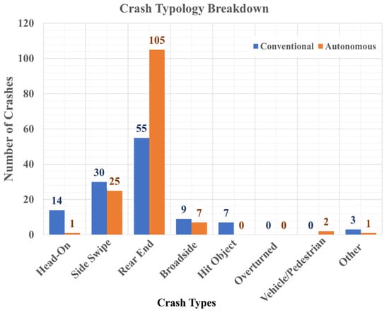
Figure 2. Crash typology distribution.

Table 3. Distribution of crash typologies, driving mode, and at-fault party.

Rear-End Crashes:	Mode		Total
	Conventional	Autonomous
Number of rear-end crashes	47	103	150
Number at fault	8	2	10
Percentage of total rear-end crash with AV at fault	5.333%	1.333%	6.667%
Sideswipe Crashes:	Mode		Total
	Conventional	Autonomous
Number of sideswipe crashes	24	23	47
Number at fault	6	2	8
Percentage of the total sideswipe crash with AV at fault	12.77%	4.26%	17.02%

Sideswipe crashes with AV on autonomous mode constitute half of the sideswipe crashes. Out of 55 sideswipe crashes, the AV was found at fault in only 8 cases. However, in 6 out of these 8 incidents, the AV was not on autonomous mode; thus, the incidents occurred while the driver was manually operating the vehicle. Rear-end collisions (62.55%) and sideswipes (20.46%) make up nearly 83.01% of recorded crashes. There are less than 5.79% (15/259) of crashes categorized as head-on. This is consistent with the previous study [5], which stated that AV technology can prevent all other crash typologies effectively, leaving rear-end collisions with AV as the most crucial failure scenario to be addressed. The Insurance Institute for Highway Safety (IIHS) notes that head-on crashes accounted for 56% of motor vehicle deaths, and 42% of deaths were caused by rear-end and side-impact accidents [36]. Thus, as AV technology can alleviate head-on collisions, it will have a positive effect on road fatality rates, a significant advantage for overall road safety.

4.2. Disengagements

Before presenting the disengagement analysis, it is essential to define some key terms. Dixit et al. (2016) stated that the AV disengagements could be initiated manually by the driver or autonomously. This distinction is crucial from a safety standpoint. Manual disengagements are cautionary in nature; for instance, if a driver feels uncomfortable in a specific situation and/or adopts a proactive approach to prevent a potential autonomous disengagement. On the other hand, automated disengagements represent a design limitation of the car and constitute a potential safety concern for the consumer and the general public. Google Inc. categorizes disengagements into two categories: Failure detection and safety operations. This study assumed that failure detection and safety operation indicate autonomous and manual disengagement, respectively. This ambiguous terminology is one of the limitations of this study; nevertheless, it is a sensible assumption for producing relevant and valuable disengagement trends.

Previous studies stated that the number of crashes observed is highly correlated with the autonomous miles travelled. The cumulative accident trend as a function of cumulative miles can reach a plateau. This plateau will signify that the AV technology training has been effective and is approaching a “crash-free” status with the more miles travelled [5]. Similar conclusions can be derived from the cumulative disengagements trend as a function of cumulative miles [6]. However, this theory can be contended as the road environment evolves with differing infrastructure, technology, and vehicle composition. More importantly, how humans interact with AVs is also changing; this is described in more detail in the following paragraph.

Figure 3 represents the plot of cumulative disengagements with cumulative miles. The blue-coloured plot represents the trend of manual disengagements, and the orange-coloured plot represents automated disengagements. The slope of the automated disengagement curve approaches zero (the curve plateaus) as the number of cumulative autonomous miles increases. Assuming that cumulative autonomous miles serve as a proxy for time/experience, we can infer that automated disengagement events are dropping and approaching zero with time/experience. Since automated disengagements indicate a design limitation and the system performance of the AV, we can infer that the system performance of AV is improving, and the AV “brain” can handle driving tasks, which were intractable before.

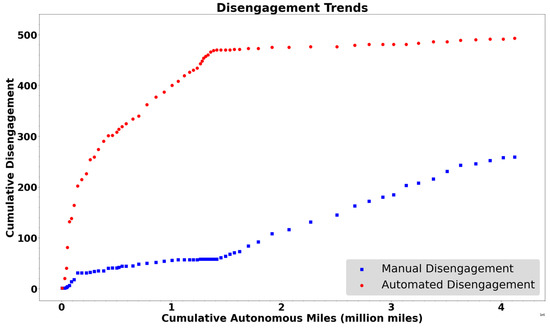
Figure 3. Disengagement trends (automated and manual).

Additionally, the non-decreasing slope of the manual disengagement curve indicates relative consistency in the degree of manual disengagement; in fact, the curve indicates that the rate of disengagement increases slightly as the cumulative autonomous miles increase. “Trust effect” can be defined as a phenomenon where the driver’s reliance on technology increases with increased miles driven, attributed to an increase in driver’s trust in the AV system [4]. Since manual disengagements initiated by the driver are cautionary in nature (manual disengagements can be potential automated disengagements that were avoided by quick and brisk action of safety operation driver), the trend implies no improvement in trust of drivers in AVs, and the “trust effect” may not be present in the light of new data. This implication is based on the conjecture that the set of potential automated disengagements and set of manual disengagements are mutually exclusive ($\mathrm{A}{{\displaystyle \cap }}^{ }\mathrm{M}=\varphi$, where A is the set of potential automated disengagements and M is the set of manual disengagements). Alternatively, the above trends can also be explained on the grounds of drivers increasing acquaintance. The underlying assumption for this implication is that a set of manual disengagements is a proper subset of potential automated disengagements ($\mathrm{M}\subseteq \mathrm{A}$). With more experience (cumulative autonomous miles) with the system, drivers can anticipate the potential intractable situations and decide to exercise caution and hence initiate manual disengagement. As a result, the number of automated disengagements decreases, despite no inordinate improvement in AV technology. Authors propose that in reality, the set of potential automated disengagements and set of manual disengagements are not mutually exclusive $\mathrm{A}{{\displaystyle \cap }}^{ }\mathrm{M}\ne \varphi$. In addition, the set of manual disengagements is not a proper subset of potential automated disengagements, and in reality, the sets are situated somewhere between two extremes. These postulations can be revised in the light of new and improved data since manufacturers are implicitly and not clearly reporting events resulting in ambiguity. A recommendation from this study is that manufacturers should provide camera and sensors data at the time of the critical event for clarity. Furthermore, the research also supports the development of a driver survey that could be issued with current reporting requirements. Ultimately, it is essential for the CA DMV to include the cause of the disengagement, given that the crash occurred after a disengagement. These recommendations were also proposed in the previous study [6]; however, this was based on a different argument. The study categorized disengagements into macro (human factors, system failures, external conditions, and others) and micro categories. The study found that Tesla’s disengagement falls under the “others” category, indicating the necessity of providing a detailed explanation. Further, the study observed that Mercedes-Benz primarily reports human factors-related disengagement and recommends other manufacturers report contributory factors. Lastly, a reporting protocol similar to what is used in the aviation industry is recommended to enhance consistency.

4.3. Models

4.3.1. Methodology and Data Brief

The crash model developed in this study considered a binary dependent variable signifying the crash and 15 independent variables which are also referred to as features. The dependent variable has two categories: 0 stands for crashes with no injury and 1 for crashes with an injury. The authors investigated the data and discovered a few complications. Firstly, all the independent variables are categorical, and the sample size corresponding to each category is small. Additionally, there is a disparity in sample size in each class. The number of samples in classes 0 (no injury) and 1 (injury) are 224 and 35, respectively. This raises the problem of skewed distributions of a binary task known as an imbalance. The total sample size is 259, with 15 explanatory variables (features) after removing rows with empty entries. The independent variables are primarily associated with the AV, other party’s vehicle, traffic conditions, and roadway features stated in the CA DMV crash reports. The Shapiro–Wilk ranking [37] was used to rank features and is presented in Figure 4a. This ranking assisted in selecting the crucial features in the model. The variable names are presented in Appendix A.2.

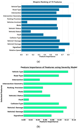
Figure 4. (a) Shapiro ranking of 15 features, (b) feature importance of features using severity model.

To handle the imbalanced data, we used stratification while dividing the data into training and testing sets. The stratification preserves the percentage of samples for each class. Two models were developed: model excluding relative velocity as a feature and model including relative velocity since the sample size is different. Out of 200 instances, only 68 instances were reported with relative velocity. The class balance of respective models is presented in Figure 5a,b. Further, we provided class weights in the models, which adjust weights inversely proportional to class frequencies in the dataset. One of the elementary ways to address the class imbalance is to provide a weight for each class. This provides more emphasis on the minority classes such that the end result is a classifier that can learn equally from all classes [38]. Class weight uses the formulae presented in Equation (1).

$$\frac{n_{sample}}{n_{classes}\times np.bincount\left(y\right) }$$

(1)

where $n_{sample}$ is the number of samples (259), $n_{classes}$ is the number of classes, and $np.bincount\left(y\right)$ counts the number of occurrences of element $y$.

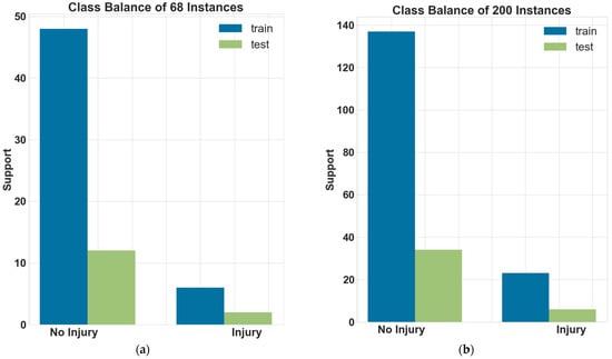
Figure 5. Class balance: (a) overall data; (b) relative velocity feature included.

The model performance is gauged by accuracy, but in the case of class imbalance, accuracy might not be the best representation of the performance of the model. Considering a user preference bias towards the minority class examples, accuracy is not suitable. If the bias is neglected, the impact of the least represented but more important examples is reduced when compared to that of the majority class [39]. Therefore, balanced accuracy is reported, which performs better with imbalanced data. False positive (FP) or type 1 error means there was an injury, but the model reported no injury, and false negative (FN) or type 2 error indicates that there was no injury recorded, but the model predicted an injury. Precision $\frac{TP}{TP+FP}$ and recall $\frac{TP}{TP+FN}$ are both important in model evaluation. Inevitably, higher values in FP can be dangerous and hence deploy more importance to the precision metric ($\frac{TP}{TP+FP}$) rather than recall. Consequently, the authors proposed to use modified F1 score similar to previous studies [40], presented in Equation (2), for evaluating the performance.

$$F_{\beta }=\left(1+{\beta }^2\right)\times \frac{precision\times recall }{{\beta }^2\times precision+recall}$$

(2)

where $F_{\beta }$ is the modified F1 score, and $\beta$ is a parameter; when 0 < β < 1, more emphasis is put on precision, and when β > 1, recall is given priority. Precision is defined as the percentage of results that is relevant, while recall is the percentage of total relevant results retrieved by the algorithm. This research uses a β of 0.5 to put more weighting on precision as it utilizes FP, and as aforementioned, FP is a crucial aspect in assessing model performance. Resampling is another technique widely used to handle imbalanced data. Khattak et al. (2020) resampled the data by oversampling the two minor classes and under-sampling the major category for balancing the dataset. However, they concluded that this dataset did not provide satisfactory results in comparison to the original data. The methodology applied for this study is presented in the flowchart shown in Figure 6. Appendix A.3 presents more information about the methodology.

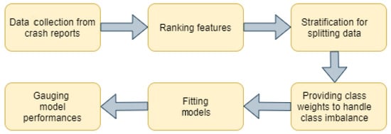
Figure 6. Methodology.

4.3.2. Crash Severity Model

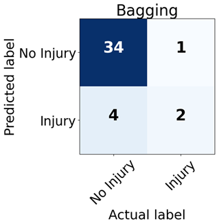
Crash severity models were developed using the DMV data and new extracted variables such as vehicle type. The most conservative model was selected as the final model. The confusion matrix and metric of the best-performing model based on modified F1 are presented in Table 4. The results for the lesser performing models used are provided in the appendix (refer to Appendix A.1). Models were developed using pre-built libraries available [41,42]. Feature importance was evaluated to rank them based on their in-model performance and is presented in Figure 4b. A bagging classifier was applied and used base estimators; in this case, the decision tree was used as a base estimator. Model-independent methods were used for computing feature importance. In the case of decision trees as base estimators, feature importance was computed by taking the average of tree’s feature importance among all trees in bagging estimators. Lastly, the precision–recall curve was used because there was a moderate to large class imbalance [43] and is presented in Appendix A.4.

Table 4. Severity model.

Confusion Matrix	Balanced Accuracy	Precision	Recall	Modified F1 Score
	0.65	0.97	0.89	0.96

Vehicle 1 damage and Vehicle 2 damage rank high in feature importance, presented in Figure 4b, which is unequivocal. It is highly likely that if the vehicles are damaged to a higher degree, the passenger might get injured. The intersection geometry and intersection management (signalization) are essential features exhibited by rank in feature importance. Additionally, 143 out of 259 rear-end crashes occurred at an intersection, and 83 of them were signalized, indicating that signalized intersections are a hotspot for crashes. As mentioned previously, an explanation could be that the percentage of amber light time translated as green by AVs and human drivers is incongruous, resulting in crashes (idealistic behaviour of AVs.). These results highlight the importance of details such as the lantern state at the time of the crash, and signal phasing should be provided within the reporting. Road type is another factor that is ranked highly. It is clear that road infrastructure elements play a crucial role in the severity and require immediate attention from a transport engineering perspective. It is further recommended that these reports also have additional information such as camera images and Lidar cloud points to assess the dynamic location characteristics such as traffic lights, parking occupancy, advertising structure, etc. Rich AV datasets available [44,45,46,47] currently fail to provide data of critical events.

Figure 7a shows the relative speed values for each category of severity. The severity categories used are the same as in the original crash reports, which are different from the developed crash severity model. The graph indicates that higher levels of severity are related to higher relative velocity values. Previous studies also showed that relative velocity is an important explanatory variable for predicting crash severity [34] and can be useful for predicting injury. Relative velocity was used as one of the explanatory variables during model formulation, but it decreased the sample size (83 instances). Out of all the manufacturers, only a few reported the relative velocity. Additionally, collision type is ranked high in feature importance. The authors recommend the CA DMV includes mandatory fields such as relative velocity, time-to-collision, and post-encroachment time to get better insights into the severity of the crashes. The non-parametric distribution was estimated using a Gaussian kernel function calculated using [48] and is presented in Figure 7b. The figure illustrates that the relative velocities during a crash are generally below 15 miles per hour (lower values), indicating less severe accidents. Consequently, another model was developed, including relative velocity as one of the explanatory variables. The training and testing data class balance is provided in Figure 5b. Logistic regression was developed using the features based on feature ranking (Figure 4) and best parameters.

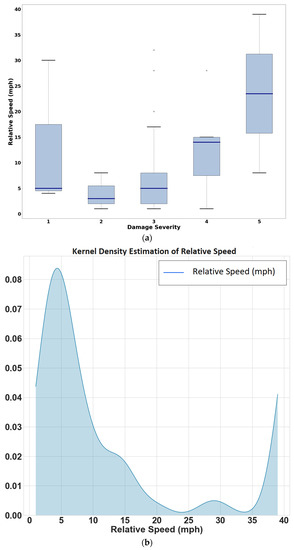
Figure 7. (a) Relative speed and accident severity, (b) probability density function (PDF) of relative velocities of vehicles during a crash.

The solver used for the model was LIBLINEAR, and the penalty was L2 [42]. The explanatory variables used were “Vehicle Type”, “Road Type”, “Intersection”, “Intersection Geometry”, “Parking Provision”, “Mode”, “Vehicle1 Status”, “Vehicle1 Damage”, “Vehicle2 Damage”, “Signalized”, and “Relative Speed”. The model performance was found to be weak with a balanced accuracy of 0.46 and confusion matrix [[11 1], [2 0]]. Further, incrementally trained logistic regression and logistic regression with cross-validation were also developed [42]. Nevertheless, these models also indicated poor model performance. As mentioned in Section 2, the severity can be gauged from three perspectives: transport viewpoint, vehicle damage viewpoint, and medical viewpoint. Relative speed is consistently considered a salient explanatory variable in all the three abovementioned assessment perspectives. Nevertheless, manufacturers are not reporting this critical variable due to optional and voluntary reporting of relative speed. Due to the lack of enough sample size, the model performed poorly when relative velocity was included.

5. Concluding Remarks and Future Work

Since automated disengagement events reduce and approach zero with time/experience, we can infer that the system performance of AV is improving, and the AV “brain” can handle driving tasks, which were intractable before. Additionally, the data reveal that there has been no reduction in manual disengagement events implying no improvement in the trust of humans with regards to AV technology. An alternate explanation for these trends is that with more experience (cumulative autonomous miles) drivers have with the system, they can anticipate the potential intractable situations better. In these scenarios, the driver decides to exercise caution and hence disengages the vehicle. With greater experience, the test drivers are actively shifting between autonomous and manual driving as they can better anticipate scenarios that AVs cannot negotiate.

Consequently, there is a decrease in automated disengagements, yet no inordinate improvement in AV technology. Additionally, increased disengagement frequency could mean that the manufacturer has broadened the conditions/scenarios in which the car is tested [6]. This explains the subsidence in plateauing in the graph of Figure 3. Using similar reasoning, it can be stated that any conclusions on technological improvement based on cumulative disengagements with cumulative miles plots are prone to indiscretion. As a result, the authors recommend averting from this approach to infer the findings of technological advancement and argue that the results in previous studies are premature. Furthermore, the authors also recommend the CA DMV includes mandatory spatial information in their reporting system.

The previous study by Xu et al. (2019) attempted to use the DMV data. The study investigated property damage only (PDO) and non-PDO crashes. They found that roadside parking, crash typology (rear-end or not), and the application of one-way roads were significant. The class imbalance of data was not considered by Xu et al. (2019), which is necessary. Additionally, the authors opine that a clear distinction between road parking provision and actual parked vehicle during the crash should be made. This was a limitation for Xu et al. (2019) and the current study. This reinforces the recommendation of appending image data at the crash locations (critical events). Additionally, further crash data must be collected to avoid any premature results due to limited data points. Consequently, the authors recommend extending this study with new data continuously collected and appended to the database.

Psychological attributes such as the risk attitude of the drivers could play a vital role in the control of AVs but are not available in the reports [49]. These would reveal other significant variables governing the damage severity. Therefore, developing a driver survey and issuing it along with the current reporting mechanism are also recommended. The crash severity field in the CA DMV reports fails to indicate the assessment outlook used to gauge severity level. The authors recommend using a specific assessment tool for potential vehicle crash damage, as stated in this study [50]. Such tools are utilitarian as their aim is to automatically make a decision for autonomous vehicles, which decide in a specific accident scenario, which type of crash is the least detrimental.

The ambiguous terminology of manual and automated disengagements because of implicit data is one of the limitations of this study. Regardless, rational assumptions are made for producing acceptable interpretations. Since the crash data are considered over a prolonged period, the time-varying explanatory variables may change significantly. Neglecting latent within-period variation may result in the loss of crucial explanatory variables. This loss of information using discrete-time intervals can institute error in model estimation because of unobserved heterogeneity [51]. Although this study provides valuable insights into AV crashes, the advancement of this technology may change the currently observed trends [14]. Additionally, using data collected over prolonged periods can also bring temporal instability to the crash severity models. The study can be improved in the future by considering temporal elements. Temporal elements can play a salient role in explaining accident trends [52]. They are typically overlooked which can lead to inaccurate and unreliable results [53]. In the future, the period for data collection can be long (over a decade). Different models can be developed for different periods instead of a single model due to temporal instability [54].

The authors identified that the available data lacked consistency. For example, crash severity levels required further processing; therefore, it is recommended that the DMV standardize data for future use.

Furthermore, improved, explicit, detailed, and increased quantities of data will inevitably produce credible and well-founded interpretations. For instance, if data from more locations (say different countries representing different driver behaviour) are available, the models could incorporate the explanatory variables such as human demographics and safety facilities (namely, medical viewpoint crash studies). This study captured the driver–AV interaction and the AV–conventional vehicle interaction. Due to limited data, it did not account for AV–AV interactions. For further investigation of the severity of AVs’ accidents, more research is required to explore AV–driver, AV–infrastructure, and driver–surrounding environment interactions, which are salient factors responsible for many crashes.

Lastly, the authors also propose that the testing location is a crucial factor that needs to be accounted for. The number of autonomous miles is a proxy for experience for a particular location. Due to the diverse nature of road infrastructure and driver behaviour in different parts of the world, it is not possible to generalize these empirical findings. It is clear from this research and that of Das et al. (2020) that there is a fundamental requirement for more advanced and robust collision narrative reporting to better assess collision likelihoods of autonomous vehicles.

Appendix A.1. Performance Comparison of Different Models

Table A1 presents the performance of different models. Bagging classifier and random forest have similar performances, and the final model is selected based on the best adjusted F1 score.

We attempted to choose the most conservative model. In this study context, false negative (type II error) is the event where there was an actual injury, but the model predicted no injury. The most conservative model should have the minimum number of false negatives. The true positives and false positives are the same in both the bagging classifier and random forest. Therefore, the final model selection was made based on false negatives, and the bagging classifier has fewer false negatives (4 < 5). Furthermore, it has a better adjusted F1 score as well.

Table A1. Performance of different models.

Models	Balanced Accuracy	Confusion Matrix				Evaluation Metric
		TP	FP	FN	TN	FPR	FDR	FOR	Precision	Recall	F1	Adjusted F1 Score
Decision Tree	0.62	32	3	4	2	0.60	0.09	0.67	0.91	0.89	0.45	0.91
Decision Tree with Weights	0.51	30	5	5	1	0.83	0.14	0.83	0.86	0.86	0.43	0.86
Bagging Classfier	0.65	34	1	4	2	0.33	0.03	0.67	0.97	0.89	0.47	0.96
Balanced Bagging Classifier	0.59	24	11	3	3	0.79	0.31	0.50	0.69	0.89	0.39	0.72
Random Forest	0.57	34	1	5	1	0.50	0.03	0.83	0.97	0.87	0.46	0.95
Balanced Random Forest Classifier	0.38	21	14	5	1	0.93	0.40	0.83	0.60	0.81	0.34	0.63
Easy Ensemble Classifier	0.73	16	19	0	6	0.76	0.54	0.00	0.46	1.00	0.31	0.51
RUSboost Classfier	0.73	22	13	1	5	0.72	0.37	0.17	0.63	0.96	0.38	0.67
Extra Trees Classifier	0.62	32	3	4	2	0.60	0.09	0.67	0.91	0.89	0.45	0.91

In the above table, TP = true positive; FP = false positive; FN = false negative; TN = true negative; FPR = false positive rate; FDR = false discovery rate; FOR = false omission rate.

Table A1. Performance of different models.

Models	Balanced Accuracy	Confusion Matrix				Evaluation Metric
		TP	FP	FN	TN	FPR	FDR	FOR	Precision	Recall	F1	Adjusted F1 Score
Decision Tree	0.62	32	3	4	2	0.60	0.09	0.67	0.91	0.89	0.45	0.91
Decision Tree with Weights	0.51	30	5	5	1	0.83	0.14	0.83	0.86	0.86	0.43	0.86
Bagging Classfier	0.65	34	1	4	2	0.33	0.03	0.67	0.97	0.89	0.47	0.96
Balanced Bagging Classifier	0.59	24	11	3	3	0.79	0.31	0.50	0.69	0.89	0.39	0.72
Random Forest	0.57	34	1	5	1	0.50	0.03	0.83	0.97	0.87	0.46	0.95
Balanced Random Forest Classifier	0.38	21	14	5	1	0.93	0.40	0.83	0.60	0.81	0.34	0.63
Easy Ensemble Classifier	0.73	16	19	0	6	0.76	0.54	0.00	0.46	1.00	0.31	0.51
RUSboost Classfier	0.73	22	13	1	5	0.72	0.37	0.17	0.63	0.96	0.38	0.67
Extra Trees Classifier	0.62	32	3	4	2	0.60	0.09	0.67	0.91	0.89	0.45	0.91

In the above table, TP = true positive; FP = false positive; FN = false negative; TN = true negative; FPR = false positive rate; FDR = false discovery rate; FOR = false omission rate.

Appendix A.2. Variables Used in the Modelling

Table A2 lists all the variables used in the modelling exercise. Details are presented in Table 2.

Table A2. Variables used in the modelling.

Vehicle Type	Vehicles Involved	Collision Type
Road Type	Mode	Vehicle1 Damage
Intersection	Vehicle1 Status	Vehicle2 Damage
Intersection Geometry	Vehicle2 Status	Signalized
Parking Provision	Fault	Relative Speed

Table A2. Variables used in the modelling.

Vehicle Type	Vehicles Involved	Collision Type
Road Type	Mode	Vehicle1 Damage
Intersection	Vehicle1 Status	Vehicle2 Damage
Intersection Geometry	Vehicle2 Status	Signalized
Parking Provision	Fault	Relative Speed

Appendix A.3. Methodology

This section provides additional details for Section 4.3.1. Skewed distributions of a binary task known as imbalance were found in the data. Stratification is used to handle the distribution of training and testing datasets and prevents sampling bias. Stratification preserves the percentage of samples for each class, which enables creating a test set with a population that best represents the original data. Sampling bias is an issue that occurs when testing a model. Model performance can be poor as test data are not representative of the whole population. Sampling bias is often observed because specific values of the variable are underrepresented or overrepresented with respect to the true distribution of the variable. Stratification, to prevent sample bias, is achieved by splitting the data into strata. The right number of instances are then sampled from each stratum to guarantee that the test set is representative of the original data. The next step is the training and development of the model. Most learning algorithms are incompetent with imbalanced data (biased class data). The training algorithm can be modified by providing different weights to the majority and minority classes. During the training, more weightage is given to the minority class in the cost function of the algorithm. Hence, it will provide a higher penalty to the minority class, and the algorithm can emphasize decreasing the errors for the minority class. Class weight uses the formulae presented in Equation (1). For our data, 259 is the number of samples ($n_{sample})$ and there are two classes ($n_{classes})$, and $np.bincount\left(y\right)$ counts the number of occurrences of element $y$. Model selection is the next step after extracting the training and testing data.

For this study, the bagging classifier was found to be the best performing model for this data. Bagging [55] is a “bootstrap” [56] ensemble method that generates individuals for its ensemble by training each classifier on a random redistribution of the training set. It fits every base classifier on random subsets of the original dataset and then aggregates their individual predictions (either by voting or by averaging) to form a final prediction. In this study, we used a decision tree as our base estimator. Each classifier’s training set is generated by randomly drawing, with replacement, N examples, where N is the size of the original training set. Each classifier in the ensemble is generated with a different random sampling of the training set. Bagging classifier can reduce overfitting. It is deployed to decrease the variance of a base estimator (e.g., a decision tree) by introducing randomization into its construction procedure and then making an ensemble out of it. Details of the basic setup of the bagging classifier are presented in Table A3.

Table A3. Basic setup parameters of the bagging classifier method.

Parameters	Assignment
Base Estimator	Decision Tree Classifier
n_estimators (the number of base estimators in th ensemble)	20
random_state	0
max_samples, max_features, bootstrap, bootstrap_features, oob_score, warm_start, n_jobs, verbose	Default values as in [42]

Table A3. Basic setup parameters of the bagging classifier method.

Parameters	Assignment
Base Estimator	Decision Tree Classifier
n_estimators (the number of base estimators in th ensemble)	20
random_state	0
max_samples, max_features, bootstrap, bootstrap_features, oob_score, warm_start, n_jobs, verbose	Default values as in [42]

Accuracy might not be the best representation of the performance model in biased class data due to user preference bias towards the minority class examples [57]. Balanced accuracy is a metric that one can use when evaluating the classifier’s performance, especially when the classes are imbalanced. Sensitivity, which is the true positive rate (also known as recall), and specificity, which is the true negative rate (also known as false positive rate), are used to define balanced accuracy. Balanced accuracy is simply the arithmetic mean of the two as presented in Equation (A1).

$$\mathrm{Balanced} \mathrm{accuracy}=\frac{\mathrm{Sensitivity}+\mathrm{Specificity}}{2}$$

(A1)

Along with balanced accuracy, a modified F1 score is also used to evaluate the model’s performance. FN indicates that there was no injury recorded, but the model predicted an injury, and FP means there was an injury, but the model reported no injury. Higher values in FP can be dangerous and hence deploy more importance to the precision instead of recall. Consequently, a modified F1 score, presented in Equation (2), is used to assess the model performance.

Appendix A.4. Precision–Recall Curve

Figure A1 presents the precision–recall curve for the bagging classifier.

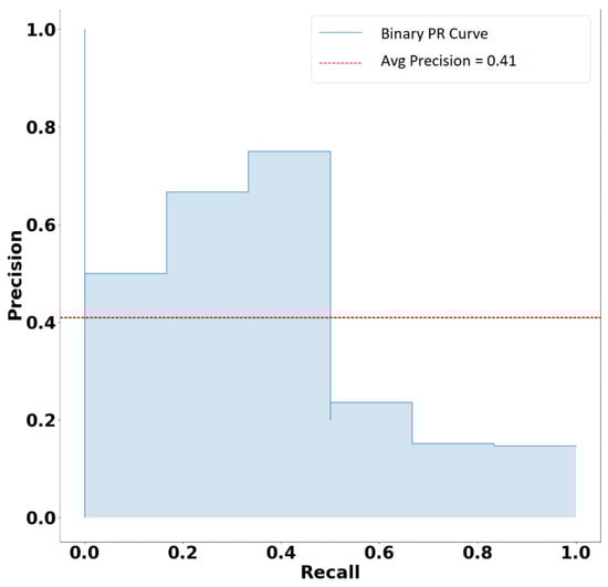
Figure A1. Precision–recall curve for bagging classifier.

References

- Taeihagh, A.; Lim, H.S.M. Governing Autonomous Vehicles: Emerging Responses for Safety, Liability, Privacy, Cybersecurity, and Industry Risks. Transp. Rev. 2019, 39, 103–128. [Google Scholar] [CrossRef] [Green Version]
- Papadoulis, A.; Quddus, M.; Imprialou, M. Evaluating the Safety Impact of Connected and Autonomous Vehicles on Motorways. Accid. Anal. Prev. 2019, 124, 12–22. [Google Scholar] [CrossRef] [Green Version]
- Sinha, A.; Chand, S.; Wijayaratna, K.P.; Virdi, N.; Dixit, V. Comprehensive Safety Assessment in Mixed Fleets with Connected and Automated Vehicles: A Crash Severity and Rate Evaluation of Conventional Vehicles. Accid. Anal. Prev. 2020, 142, 105567. [Google Scholar] [CrossRef]
- Dixit, V.V.; Chand, S.; Nair, D.J. Autonomous Vehicles: Disengagements, Accidents and Reaction Times. PLoS ONE 2016, 11, e0168054. [Google Scholar] [CrossRef] [Green Version]
- Favarò, F.M.; Nader, N.; Eurich, S.O.; Tripp, M.; Varadaraju, N. Examining Accident Reports Involving Autonomous Vehicles in California. PLoS ONE 2017, 12, e0184952. [Google Scholar] [CrossRef]
- Favarò, F.; Eurich, S.; Nader, N. Autonomous Vehicles’ Disengagements: Trends, Triggers, and Regulatory Limitations. Accid. Anal. Prev. 2018, 110, 136–148. [Google Scholar] [CrossRef] [PubMed]
- Favarò, F.M.; Eurich, S.O.; Rizvi, S.S. “Human” Problems in Semi-Autonomous Vehicles: Understanding Drivers’ Reactions to Off-Nominal Scenarios. Int. J. Hum. Comput. Interact. 2019, 35, 956–971. [Google Scholar] [CrossRef]
- Banerjee, S.S.; Jha, S.; Cyriac, J.; Kalbarczyk, Z.T.; Iyer, R.K. Hands Off the Wheel in Autonomous Vehicles?: A Systems Perspective on over a Million Miles of Field Data. In Proceedings of the 48th Annual IEEE/IFIP International Conference on Dependable Systems and Networks (DSN), Luxembourg, 25–28 June 2018; pp. 586–597. [Google Scholar]
- Khattak, Z.H.; Fontaine, M.D.; Smith, B.L. Exploratory Investigation of Disengagements and Crashes in Autonomous Vehicles under Mixed Traffic: An Endogenous Switching Regime Framework. IEEE Trans. Intell. Transp. Syst. 2020, 1–11. [Google Scholar] [CrossRef]
- Boggs, A.M.; Wali, B.; Khattak, A.J. Exploratory Analysis of Automated Vehicle Crashes in California: A Text Analytics & Hierarchical Bayesian Heterogeneity-Based Approach. Accid. Anal. Prev. 2020, 135, 105354. [Google Scholar] [CrossRef] [PubMed]
- Wang, J.; Zhang, L.; Huang, Y.; Zhao, J. Safety of Autonomous Vehicles. J. Adv. Transp. 2020, 2020, e8867757. [Google Scholar] [CrossRef]
- Das, S.; Dutta, A.; Tsapakis, I. Automated Vehicle Collisions in California: Applying Bayesian Latent Class Model. IATSS Res. 2020, 44, 300–308. [Google Scholar] [CrossRef]
- Xu, C.; Ding, Z.; Wang, C.; Li, Z. Statistical Analysis of the Patterns and Characteristics of Connected and Autonomous Vehicle Involved Crashes. J. Saf. Res. 2019, 71, 41–47. [Google Scholar] [CrossRef]
- Khattak, Z.H.; Fontaine, M.D.; Smith, B.L. An Exploratory Investigation of Disengagements and Crashes in Autonomous Vehicles. In Proceedings of the Transportation Research Board 98th Annual Meeting, Washington, DC, USA, 13–17 January 2019. [Google Scholar]
- Sobhani, A.; Young, W.; Logan, D.; Bahrololoom, S. A Kinetic Energy Model of Two-Vehicle Crash Injury Severity. Accid. Anal. Prev. 2011, 43, 741–754. [Google Scholar] [CrossRef]
- Zeng, Q.; Hao, W.; Lee, J.; Chen, F. Investigating the Impacts of Real-Time Weather Conditions on Freeway Crash Severity: A Bayesian Spatial Analysis. Int. J. Environ. Res. Public Health 2020, 17, 2768. [Google Scholar] [CrossRef]
- Cheng, W.; Gill, G.S.; Sakrani, T.; Dasu, M.; Zhou, J. Predicting Motorcycle Crash Injury Severity Using Weather Data and Alternative Bayesian Multivariate Crash Frequency Models. Accid. Anal. Prev. 2017, 108, 172–180. [Google Scholar] [CrossRef] [PubMed]
- Holdridge, J.M.; Shankar, V.N.; Ulfarsson, G.F. The Crash Severity Impacts of Fixed Roadside Objects. J. Saf. Res. 2005, 36, 139–147. [Google Scholar] [CrossRef]
- Quddus, M.A.; Wang, C.; Ison, S.G. Road Traffic Congestion and Crash Severity: Econometric Analysis Using Ordered Response Models. J. Transp. Eng. 2009, 136, 424–435. [Google Scholar] [CrossRef]
- Olia, A.; Razavi, S.; Abdulhai, B.; Abdelgawad, H. Traffic Capacity Implications of Automated Vehicles Mixed with Regular Vehicles. J. Intell. Transp. Syst. 2018, 22, 244–262. [Google Scholar] [CrossRef]
- Virdi, N.; Grzybowska, H.; Waller, S.T.; Dixit, V. A Safety Assessment of Mixed Fleets with Connected and Autonomous Vehicles Using the Surrogate Safety Assessment Module. Accid. Anal. Prev. 2019, 131, 95–111. [Google Scholar] [CrossRef]
- Buzeman, D.G.; Viano, D.C.; Lövsund, P. Injury Probability and Risk in Frontal Crashes: Effects of Sorting Techniques on Priorities for Offset Testing. Accid. Anal. Prev. 1998, 30, 583–595. [Google Scholar] [CrossRef]
- Rana, T.A.; Sikder, S.; Pinjari, A.R. Copula-Based Method for Addressing Endogeneity in Models of Severity of Traffic Crash Injuries: Application to Two-Vehicle Crashes. Transp. Res. Rec. 2010, 2147, 75–87. [Google Scholar] [CrossRef]
- Farmer, C.M.; Braver, E.R.; Mitter, E.L. Two-Vehicle Side Impact Crashes: The Relationship of Vehicle and Crash Characteristics to Injury Severity. Accid. Anal. Prev. 1997, 29, 399–406. [Google Scholar] [CrossRef]
- Huelke, D.F.; Compton, C.P. The Effects of Seat Belts on Injury Severity of Front and Rear Seat Occupants in the Same Frontal Crash. Accid. Anal. Prev. 1995, 27, 835–838. [Google Scholar] [CrossRef]
- Bédard, M.; Guyatt, G.H.; Stones, M.J.; Hirdes, J.P. The Independent Contribution of Driver, Crash, and Vehicle Characteristics to Driver Fatalities. Accid. Anal. Prev. 2002, 34, 717–727. [Google Scholar] [CrossRef]
- Carbaugh, J.; Godbole, D.N.; Sengupta, R. Safety and Capacity Analysis of Automated and Manual Highway Systems. Transp. Res. Part C Emerg. Technol. 1998, 6, 69–99. [Google Scholar] [CrossRef] [Green Version]
- Langley, J.; Marshall, S.W. The Severity of Road Traffic Crashes Resulting in Hospitalisation in New Zealand. Accid. Anal. Prev. 1994, 26, 549–554. [Google Scholar] [CrossRef]
- Conroy, C.; Tominaga, G.T.; Erwin, S.; Pacyna, S.; Velky, T.; Kennedy, F.; Sise, M.; Coimbra, R. The Influence of Vehicle Damage on Injury Severity of Drivers in Head-on Motor Vehicle Crashes. Accid. Anal. Prev. 2008, 40, 1589–1594. [Google Scholar] [CrossRef]
- Lee, J.; Conroy, C.; Coimbra, R.; Tominaga, G.T.; Hoyt, D.B. Injury Patterns in Frontal Crashes: The Association between Knee–Thigh–Hip (KTH) and Serious Intra-Abdominal Injury. Accid. Anal. Prev. 2010, 42, 50–55. [Google Scholar] [CrossRef]
- Bainbridge, L. Ironies of Automation. In Analysis, Design and Evaluation of Man–Machine Systems; Johannsen, G., Rijnsdorp, J.E., Eds.; Pergamon: Oxford, UK, 1983; pp. 129–135. ISBN 978-0-08-029348-6. [Google Scholar]
- Wiener, B.E.L.; Curry, R.E. Flight-Deck Automation: Promises and Problems. Ergonomics 1980, 23, 995–1011. [Google Scholar] [CrossRef]
- Corben, B.; Senserrick, T.; Cameron, M.; Rechnitzer, G. Development of the Visionary Research Model: Application to the Car/Pedestrian Conflict; Monash University Accident Research Centre: Melbourne, Australia, 2004. [Google Scholar]
- Elvik, R. To What Extent Can Theory Account for the Findings of Road Safety Evaluation Studies? Accid. Anal. Prev. 2004, 36, 841–849. [Google Scholar] [CrossRef]
- Papaioannou, P. Driver Behaviour, Dilemma Zone and Safety Effects at Urban Signalised Intersections in Greece. Accid. Anal. Prev. 2007, 39, 147–158. [Google Scholar] [CrossRef]
- The Insurance Institute for Highway Safety (IIHS). Fatality Facts 2019: Passenger Vehicle Occupants. Available online: https://www.iihs.org/topics/fatality-statistics/detail/passenger-vehicle-occupants (accessed on 25 June 2021).
- Shapiro, S.S.; Wilk, M.B. An Analysis of Variance Test for Normality (Complete Samples). Biometrika 1965, 52, 591–611. [Google Scholar] [CrossRef]
- Jordan, J. Learning from Imbalanced Data. Available online: https://www.jeremyjordan.me/imbalanced-data/ (accessed on 25 June 2021).
- Branco, P.; Torgo, L.; Ribeiro, R.P. A Survey of Predictive Modeling on Imbalanced Domains. ACM Comput. Surv. 2016, 49, 1–50. [Google Scholar] [CrossRef]
- Li, Z.; Chen, W.; Pei, D. Robust and Unsupervised KPI Anomaly Detection Based on Conditional Variational Autoencoder. In Proceedings of the 2018 IEEE 37th International Performance Computing and Communications Conference (IPCCC), Orlando, FL, USA, 17–19 November 2018; pp. 1–9. [Google Scholar]
- Lemaître, G.; Nogueira, F.; Aridas, C.K. Imbalanced-Learn: A Python Toolbox to Tackle the Curse of Imbalanced Datasets in Machine Learning. J. Mach. Learn. Res. 2017, 18, 559–563. [Google Scholar]
- Pedregosa, F.; Varoquaux, G.; Gramfort, A.; Michel, V.; Thirion, B.; Grisel, O.; Blondel, M.; Prettenhofer, P.; Weiss, R.; Dubourg, V.; et al. Scikit-Learn: Machine Learning in Python. J. Mach. Learn. Res. 2011, 12, 2825–2830. [Google Scholar]
- Saito, T.; Rehmsmeier, M. The Precision-Recall Plot Is More Informative than the ROC Plot When Evaluating Binary Classifiers on Imbalanced Datasets. PLoS ONE 2015, 10, e0118432. [Google Scholar] [CrossRef] [PubMed] [Green Version]
- Caesar, H.; Bankiti, V.; Lang, A.H.; Vora, S.; Liong, V.E.; Xu, Q.; Krishnan, A.; Pan, Y.; Baldan, G.; Beijbom, O. NuScenes: A Multimodal Dataset for Autonomous Driving. In Proceedings of the IEEE/CVF Conference on Computer Vision and Pattern Recognition, Seattle, WA, USA, 13–19 June 2020; pp. 11621–11631. [Google Scholar]
- Maddern, W.; Pascoe, G.; Linegar, C.; Newman, P. 1 Year, 1000 Km: The Oxford RobotCar Dataset. Int. J. Robot. Res. 2017, 36, 3–15. [Google Scholar] [CrossRef]
- Huang, X.; Cheng, X.; Geng, Q.; Cao, B.; Zhou, D.; Wang, P.; Lin, Y.; Yang, R. The ApolloScape Dataset for Autonomous Driving. In Proceedings of the IEEE Computer Society Conference on Computer Vision and Pattern Recognition Workshops (CVPRW), Salt Lake City, UT, USA, 18–22 June 2018; pp. 954–960. [Google Scholar]
- Sun, P.; Kretzschmar, H.; Dotiwalla, X.; Chouard, A.; Patnaik, V.; Tsui, P.; Guo, J.; Zhou, Y.; Chai, Y.; Caine, B. Scalability in Perception for Autonomous Driving: Waymo Open Dataset. In Proceedings of the IEEE/CVF Conference on Computer Vision and Pattern Recognition, Seattle, WA, USA, 13–19 June 2020; pp. 2446–2454. [Google Scholar]
- Terrell, G.R.; Scott, D.W. Variable Kernel Density Estimation. Ann. Stat. 1992, 20, 1236–1265. [Google Scholar] [CrossRef]
- Dixit, V.; Xiong, Z.; Jian, S.; Saxena, N. Risk of Automated Driving: Implications on Safety Acceptability and Productivity. Accid. Anal. Prev. 2019, 125, 257–266. [Google Scholar] [CrossRef]
- Wiseman, Y.; Grinberg, I. Circumspectly Crash of Autonomous Vehicles. In Proceedings of the 2016 IEEE International Conference on Electro Information Technology (EIT), Grand Forks, ND, USA, 19–21 May 2016; pp. 0387–0392. [Google Scholar]
- Washington, S.P.; Karlaftis, M.G.; Mannering, F. Statistical and Econometric Methods for Transportation Data Analysis; CRC Press: Boca Raton, FL, USA, 2010. [Google Scholar]
- Mannering, F. Temporal Instability and the Analysis of Highway Accident Data. Anal. Methods Accid. Res. 2018, 17, 1–13. [Google Scholar] [CrossRef]
- Al-Bdairi, N.S.S.; Behnood, A.; Hernandez, S. Temporal Stability of Driver Injury Severities in Animal-Vehicle Collisions: A Random Parameters with Heterogeneity in Means (and Variances) Approach. Anal. Methods Accid. Res. 2020, 26, 100120. [Google Scholar] [CrossRef]
- Theofilatos, A.; Antoniou, C.; Yannis, G. Exploring Injury Severity of Children and Adolescents Involved in Traffic Crashes in Greece. J. Traffic Transp. Eng. 2020. [Google Scholar] [CrossRef]
- Breiman, L. Bagging Predictors. Mach. Learn. 1996, 24, 123–140. [Google Scholar] [CrossRef] [Green Version]
- Efron, B.; Tibshirani, R.J. An Introduction to the Bootstrap; CRC Press: Boca Raton, FL, USA, 1994; ISBN 978-0-412-04231-7. [Google Scholar]
- Branco, P.; Torgo, L.; Ribeiro, R. A Survey of Predictive Modelling under Imbalanced Distributions. arXiv 2015, arXiv:1505.01658. [Google Scholar]
Publisher’s Note: MDPI stays neutral with regard to jurisdictional claims in published maps and institutional affiliations. |
© 2021 by the authors. Licensee MDPI, Basel, Switzerland. This article is an open access article distributed under the terms and conditions of the Creative Commons Attribution (CC BY) license (https://creativecommons.org/licenses/by/4.0/).