Abstract
This study investigates the impact of income inequality on household carbon emissions in China using nationwide micro panel data. The effect is positive—households in counties with greater income inequality emit more—and remarkably robust to a battery of robustness checks. We also explore the roles that consumption patterns, time preference, and mental health play in the relationship between income inequality and household carbon emissions. The findings suggest that the change in consumption patterns caused by income inequality may be an important reason for the positive effect of inequality on household carbon emissions and that a lower time preference for consumption and improved mental health can mitigate the positive effect of income inequality on household carbon emissions. Furthermore, substantial differences are found among households at different income levels and households with heads of different ages. The findings of this study provide important insights for policy makers to reduce both inequality and emissions.
1. Introduction
Global warming caused by greenhouse gases (GHGs), a catastrophic threat to human survival and development, has incited worldwide concern [1]. In the last decade from 2009 to 2018, total GHG emissions grew by 1.5 percent per year without land-use change (LUC), and the top four emitters (China, EU28, India and the United States of America) contribute over 55 percent of the total GHG emissions excluding LUC [2]. Carbon dioxide (CO2) is a leading source of GHGs [3]. The global average annual concentration of carbon dioxide in the atmosphere averaged 407.4 ppm in 2018; however, the pre-industrial levels only ranged between 180 and 280 ppm (International Energy Agency, IEA).
In the past 40 years, the world has witnessed the rapid development of China’s economy as well as the increase of carbon emissions. According to statistics from the Oak Ridge National Laboratory Carbon Dioxide Information Analysis Center (CDIAC), China became the world’s largest carbon emitter in 2008, with carbon emissions increased from 2.089 billion metric tons in 1990 to 9.258 billion metric tons in 2017, accounting for approximately 28.2% of the world’s total emissions [4]. This fact has brought China tremendous international pressures for emission reduction. Therefore, to cope with the challenges of climate change and achieve sustainable development, the Chinese government announced its intention to reduce emissions per unit of gross domestic product to 60%–65% from the 2005 levels and to reach peak GHG emissions by 2030 in the Paris Agreement [5,6]. To accomplish this ambitious goal, China has to make a combination of various efforts, and household emission reduction will contribute significantly. In fact, the household sector should be responsible for a major part of the carbon emissions of an economy [7]. The household sector accounts for more than 80% of carbon emissions in the United States [8] and exceeds 70% in the United Kingdom and India [9,10]. Liu et al. (2011) found that in China, the share of emissions from household sector was approximately 40% of the total [11], and Fan et al. (2013) found that the annual growth rate of household carbon emissions in China was 8.7% [12]. Although the industrial sector remains the key source of carbon emissions, as a demander of industrial products, the household sector indirectly promotes CO2 emissions [13,14], and in China, the residential sector has become the second largest CO2 emissions source [15]. This fact emphasizes the importance of placing greater attention on household carbon emissions.
In addition to environmental degradation, the increasing income inequality, as a by-product of economic growth, is also an important socio-economic issue [16,17]. Income inequality may cause substantial social and economic problems, such as poorer mental health [18,19], higher status anxiety [20], and a higher level of general violence [21]. Furthermore, income inequality will create highly indebted, low-income households, which eventually results in a fragile economy [22]. China’s economy has made remarkable achievements since its reform and opening up, but the fruits of economic growth are not shared equally among the population [23]. The Gini coefficient of income distribution in China increased by 55% between 1974 and 2010 [24], and in 2017, it reached 0.467 (China Yearbook of Household Survey), exceeding the warning level of 0.40 set by the United Nations. A series of fiscal and tax policies have been adopted to regulate income distribution. One question deserving attention is whether under the dual pressures of environment and inequality, the policy goal of narrowing the income gap consistent with the carbon reduction target. In particular, does income inequality itself lead to the increase of carbon emissions [25]?
Different from previous studies, this paper focuses on the effect of income inequality on carbon emissions of households at similar income levels; that is to say, we explore whether households at similar income levels emit differently when facing different levels of income inequality. More specifically, we use three waves of data at the household level, from the China Family Panel Survey (CFPS, downloadable at http://www.isss.pku.edu.cn/cfps/), to estimate the influence of income inequality on household carbon emissions and to examine consumption patterns, mental health and time preference for consumption as important channels through which income inequality influences household emissions.
The present paper may contribute to the literature in three ways. First, we test the relationship between income inequality and household carbon emissions in China; here, we diverge from a large body of the existing literature on the differences of emissions among households at different income levels to focus on the emissions of households at similar income levels when facing different levels of income inequality. Although there is a general perception that households at different income levels emit differently, it is unclear how households with similar income act when facing different income inequality levels. Second, we explore the mechanisms by which income inequality affects household CO2 emissions. Subjective factors such as mental health and time preference for consumption, in addition to consumption patterns, allow us to offer some new insights into this topic. Third, our findings suggest that with the increase of the age of household heads and the increase of households’ per capita income, the positive effect of income inequality on household carbon emissions gradually decreases. This result suggests a new approach for the government to formulate more precise income distribution and emission reduction policies.
2. Literature Review
Boyce (1994) performed the pioneering work of incorporating inequality into environmental degradation and argued that greater inequalities in power and wealth led to worse environmental quality [26]. Boyce presented a political-economic explanation that, on the one hand, the wealthy preferred weaker environmental protection policies because they reaped disproportionate gains from pollution, while on the other hand, inequality increased the preference for current resource consumption of both the poor and the rich. However, this argument holds only in the assumption that the rich prefer more pollution than the poor [27,28]. Ravallion et al. (2000), Heil and Selden (2001), and Borghesi (2006) explained the relationship between income inequality and carbon emissions from the perspective of “marginal propensity to emit” (MPE) [29,30,31]; however, they did not obtain accordant conclusions. In line with Boyce’s point of view, studies relying on individual economic behavior suggest that increasing inequality in income will increase CO2 emissions. Not only the wealthy but also the poor will engage in expensive and conspicuous consumption to maintain or obtain a higher social status, which Schor (1998) and Veblen (2009) described as the “Veblen effect” [32,33].
There are also many empirical studies, but unfortunately, no consensus on the relationship between income inequality and carbon emissions has been reached. Golley and Meng (2012), Baek and Gweisah (2013), Jorgenson (2015), Kasuga and Takaya (2017), Liu et al. (2019), and Uzar and Eyuboglu (2019) came to the conclusion that higher CO2 emissions were positively associated with increasing income inequality [34,35,36,37,38,39]. In contrast, Heerink et al. (2001), Coondoo and Dinda (2008), Baloch et al. (2017), Hübler (2017), and Sager (2019) held that inequality affected carbon emissions in the opposite direction [28,40,41,42,43]. Using an unbalanced panel data set from 158 countries, Grunewald et al. (2017) found that the impact of income inequality on carbon emissions varied with economic development levels [44]. For low- and middle-income economies, higher levels of income inequality helped reduce emissions, while in upper middle-income and high-income economies, higher levels of income inequality increased emissions. Jorgenson et al. (2017) studied the influence of income inequality, measured with the income share of the top 10% and the Gini coefficient, on state-level CO2 emissions of the United States [25]. They found a positive relationship between inequality and carbon emissions, but the relationship was only significant when income inequality was measured with the income share of the top 10%. Liu et al. (2019), for the first time, took the short- and long-term impacts of income inequality on CO2 into consideration [38]. They suggested that higher income inequality increased carbon emissions in the short term, but in the long term, it promoted carbon reduction. There are even studies finding no linkage between income inequality and environmental quality [45,46].
Some studies found that income anticipations could affect mental health and that income inequality generally damaged subjective well-being and led to psychological problems [18,47,48,49,50,51]. Further, Velek and Steg (2007) proposed that psychological factors were important in promoting sustainable consumption of natural resources [52]. Kaida and Kaida (2016) found that pro-environmental behavior was positively associated with present subjective well-being [53]. Koenig-Lewis et al. (2014) tested 312 Norwegian consumers on their evaluation of a beverage container incorporating organic material [54]. They suggested that emotions and rationality drove pro-environmental purchasing behavior, and positive emotion was a significant predictor of green product purchases. Bissing-Olson et al. (2016) examined the dynamic interplay between everyday emotions and pro-environmental behavior over time, and their findings showed that whether individuals felt pride or guilt had an impact on the related pro-environmental behaviors during the course of their day [55]. Ibanez et al. (2017) reported that awe fostered solemnity and heightened analytical ability, which in turn affected individuals’ pro-environmental behavior [56]. A recent study by Li et al. (2019) using the China Household Finance Survey (CHFS) also found that feeling happy caused a decrease in energy consumption and thus reduced household carbon emissions [57].
Based on these discussions, it is clear that most of the existing literature investigates the effect of income inequality on carbon emissions focused on the national level, state level, or city level; however, few studies concern about the micro behavior body: the households. Based on the United States Consumer Expenditure Survey (CEX) from 1996 to 2009, Sager (2019) estimated the Environmental Engel curves (EECs) and examined the effects of different factors on the evolution of carbon emissions over time [43]. He found that income, age structure, education, family size, race, and region were relevant, and among these factors, income played a major role. Using the data from China’s Urban Household Income and Expenditure Survey (UHIES) in 2005, Golley and Meng (2012) investigated variations in household CO2 emissions among households at different income levels [34]. They demonstrated that rich households emitted more than poor households and that marginal propensity to emit (MPE) slightly increased with income over the relevant income range. Therefore, they concluded that the redistribution of income from the rich to the poor could reduce aggregate household emissions. More importantly, studies rarely consider the differences in carbon emissions among households at similar income levels, and few studies focus on the relationship between income inequality and household carbon emissions from the perspective of psychology.
3. Data Source and Empirical Methodology
Using the consumption lifestyle approach (CLA), we first calculate household carbon emissions by consumption category, which is the dependent variable of this paper but cannot be obtained directly from the CFPS. Then we estimate the Gini coefficient of each county as the proxy variable of income inequality. In the empirical section, we employ fixed-effects estimation to reveal the causal relationship between income inequality and household carbon emissions.
3.1. Data Source
This study adopts panel data from China Family Panel Survey (CFPS) administered by Institute of Social Science Survey, Peking University. The CFPS is a nationally representative survey of Chinese communities, families, and individuals. This dataset provides a high-quality comprehensive survey of household income, expenditure, subjective attitudes, and other demographic characteristics. The CFPS was launched in 2010, commenced with a total of 14,960 households from 635 communities, including 33,600 adults and 8990 youths, located in 25 provinces (excluding Tibet, Xinjiang, Inner Mongolia, Hainan, Ningxia, Qing Hai, Hong Kong, Macao, and Taiwan). Because there are lots of defaults in subjective attitude, which is important for mechanism analysis, in the fourth round of the CFPS in 2016, we use the first three rounds of the survey, conducted in 2010, 2012, and 2014, respectively.
3.1.1. Household Carbon Emissions
According to Wei et al. (2007), household carbon emissions include indirect emissions and direct emissions [58]. The indirect carbon emissions are from the following seven consumption categories: (1) food, (2) clothing, (3) household facilities, articles, and services, (4) medicine and medical services, (5) transportation and communication services, (6) education, cultural and recreation services, and (7) miscellaneous commodities and services. The direct carbon emissions are from residential use of electricity, fuel, and other utilities. Following the approach of Li et al. (2019), we calculate household carbon emissions by multiplying the monetary expenditure in each expenditure category by the respective emissions conversion coefficient [57]:
where is carbon emissions of the household caused by category, is the vector of direct emissions intensity in each production sector, and is the domestic Leontief inverse matrix, is the spending in the category by the household, is total carbon emissions of the household. Because China reports the input-output table every five years and the most recent report that is available to us is from 2012, we calculate the carbon intensity coefficients for each consumption category based on the China Input-Output Table in 2012 and sectoral carbon emissions data from the China Emission Accounts and Datasets (downloadable at: http://www.stats.gov.cn/ztjc/tjzdgg/trccxh/zlxz/trccb/201701/t201701131453448.html) in 2012 over the three years. The expenditures and income values for 2012 and 2014 are adjusted to constant 2010 prices according to the CPI indices published by the National Bureau of Statistics (NBS). Following Su and Ang (2015) and Li et al. (2019), we use the non-competitive imports assumption to account for the embodied emissions from domestic production [57,59].
Because expenditure on miscellaneous commodities and services is generally very small in number and there is no detailed expenditure information on miscellaneous commodities and services in the CFPS, this paper does not consider the emissions of this category. Figure 1 plots a histogram of the average household carbon emissions by consumption category in 2010, 2012, and 2014, respectively. We find that the residential use, food, education, culture and recreation services are the first three categories in inducing carbon emissions, and the residential use produces most of the total emissions with a proportion of 53.88% in 2010, 53.93% in 2012, and 77.68% in 2014. A great deal of literature documents that different consumption patterns of households in different income levels cause a positive/negative impact of income equality on household carbon emissions [60]. Therefore, we further aggregate the households in the CFPS into five groups according to the principle of classification of the NBS and calculate the carbon emissions of different income groups by category. As shown in Figure 2, carbon emissions generated by household facilities, articles and services, transportation and communication services, and residential use are more in richer households, especially in 2010 and 2012, and these three categories are considered to be high carbon-intensive mix [61]. In 2014, the carbon emissions generated by residential use increased a lot in all income groups, compared with the previous two years. We can also clearly see that poorer households spend more on medicine and medical services. Taking year 2010 as an example, the proportion of carbon emissions caused by medicine and medical services of the income groups from the 1st to the 5th are about 16.20%, 12.79%, 8.07%, 8.07%, 5.29%, respectively.
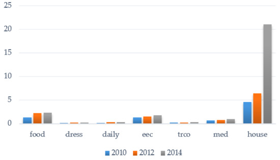
Figure 1.
Household carbon emissions by consumption category in China: Y-axis is the average household carbon emissions of each consumption category. X-axis is consumption categories, where “food” refers to expenditure on food, “dress” refers to expenditure on clothing, “daily” refers to expenditure on household facilities, articles, and services, “eec” refers to expenditure on education, cultural and recreation services, “trco” refers to expenditure on transportation and communication services, “med” refers to expenditure on medicine and medical services, “house” refers to expenditure on residential use.
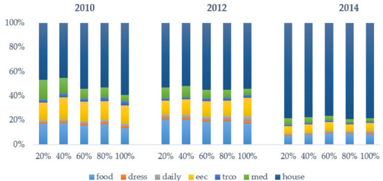
Figure 2.
Carbon emissions of different income groups by consumption category: Y-axis is the proportion of average household carbon emissions of each consumption category. X-axis is households in different income groups.
3.1.2. Income Inequality
Following Liu et al. (2019), we apply the Gini coefficient to proxy the income inequality within a given county [62]. The specific formula is as follows:
where denotes the county-level Gini coefficient; is the number of households; refers to the average per capita income of all households. and represent the per capita income of household and household , respectively. The values of estimated Gini coefficients can range from zero (perfect equality) to 1 (perfect inequality).
Figure 3 shows the income inequality distribution of China based on the estimated sample of CFPS in 2010, 2012, and 2014. There are many counties with the Gini coefficient exceeding the warning value of 0.4 (73.5% in 2010, 76.1% in 2012, 71.6% in 2014), which indicates that the income inequality is at a high level in China. This is consistent with the results published by the NBS: the national Gini coefficients in 2010, 2012, and 2014 are 0.481, 0.474, and 0.469, respectively.
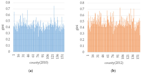
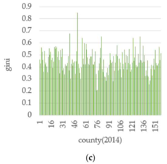
Figure 3.
County-level income inequality based on households’ per capita income: Y-axis is the Gini coefficients. X-axis is county numbers. (a) is the Gini coefficients at county-level of 2010, (b) is the Gini coefficients at county-level of 2012, and (c) is the Gini coefficients at county-level of 2014.
3.1.3. Descriptive Statistics
In all empirical tests, we control the household characteristics, demographic characteristics of the head of the household, and social and economic factors. Table 1 reports the definitions and descriptive statistics of the variables. The average carbon emissions of Chinese households are 6.905, 10.096, 24.142 tons in 2010, 2012, and 2014, respectively, which reveals that household carbon emissions are increasing during the investigating period. Meanwhile, we find that household carbon emissions are also unequal because there is a great value of Standard Deviation especially in 2014. The average Gini coefficients are 0.437, 0.495, and 0.453 in 2010, 2012, and 2014, respectively.

Table 1.
Variable descriptions and descriptive statistics.
We control the demographic characteristics of the head of each household, including age [63], gender [64,65], marital status, hukou (hukou is a unique household registration system in China, and under this system, all people are divided into residents with urban hukou and residents with rural hukou; generally, people with different hukou enjoy different welfare benefits), policy [57], years of education [66,67], and self-reported health.
We use the proportion of members of a household who are working, child dependency ratio, elderly dependency ratio, family size, car ownership, dwelling size, household per capita income, and household net wealth to control the household characteristics, and the distance to county center, residence location (urban or rural), economic status, and building density to control the community characteristics. The age composition of a household has an impact on energy use and carbon emissions [34,68]. Family size is an important factor in household carbon footprints [69]. Meier and Rehdanz (2010) found that heating expenditure increased with household size [70]. Similarly, households with at least one car and a larger dwelling size will produce more emissions because they need more energy [57]. Many studies show that income is the predominant determinant explaining in the increase of household carbon emissions, such as Dong and Zhao (2017), Ottelin et al. (2018), and Qu et al. (2019) [15,71,72]. Compared with rural households, urban households consume more processed products, and more complicated processing program may cause more carbon emissions. Household carbon emissions relate to spatial development, and building density is a non-negligible factor [73,74].
3.2. The Econometric Model
This study relies on a panel regression model, which we used to analyze the relationship between income inequality and household CO2 emissions. We construct a model of household CO2 emissions as follows:
where , and denote the household, county, and year, respectively; represents CO2 emissions of the household; is the income inequality measured by Gini coefficient at the county level; is a vector of control variables that includes the demographic characteristics of the heads of households, household characteristics, and community characteristics.
4. Empirical Results
This section presents the regression results. We first report the baseline results to show how income inequality on the county-level affects household carbon emissions. We use a fixed-effects method to test Model (4), and use Lewbel (2012) two-stage least squares method to solve the endogenous problem [75]. We make a series of robustness tests. Then, the interaction terms are introduced into the basic model to reveal the underlying mechanisms. Finally, we examine the heterogeneity of income inequality affecting household carbon emissions.
4.1. Baseline Results
Columns (1), (2), (3) and (4) of Table 2 reports the estimation results with respect to different control variables according to Model (4). There is only the core explanatory variable, the Gini coefficient, in Column (1). Column (2) includes the controlling variables of the demographic characteristics of the household head, and in Column (3), we further add the household characteristics. In Column (4), the Gini coefficient is included along with all of the controlling variables.
Table 2.
Baseline Regression results of the effect of income inequality on household CO2 emissions in China.
As seen, the results paint a consistent picture. The coefficients on income inequality are significant and positive in all of the columns, (1), (2), (3) and (4), implying that household carbon emissions increase with income inequality at the county level, which is in accordance with Liu et al. (2019) and Uzar and Eyuboglu (2019) [39,62]. Specifically, a one-standard-deviation increase in the Gini coefficient will increase household carbon emissions by 6%. This result demonstrates that income inequality in a region have a strong negative impact on pro-environmental behavior. Indeed, improving income inequality improves the social stability, and this additional value is crucial for general sustainable development in China.
The results of other control variables are generally consistent with our expectations. For example, women are more environmentally friendly than men [76,77]. A larger household emits more because it consumes more energy [70], and households with at least one car produce more emissions than households without a car, as the former consume more fuel for driving [57]. Households at a higher income level have a stronger purchasing power, which leads to an increase in demand for home comforts and, in turn, induces more CO2 emissions [78,79]. Households located in urban areas produce more carbon emissions [57].
A common view is that older people tend to generate more CO2 emissions [34,68]; however, we find otherwise. The older generations have experienced difficult times, and this experience forms in them a frugal consumption habit. Few studies have investigated the role of health in carbon emissions. Given that health care contributes abundant total emissions, this paper takes the health status of the heads of households into consideration. We find that a household with a healthy head emits less than one with an unhealthy head.
Although we use a fixed-effects model to control for missing variables that do not change with time at the household level, there are still some unobservable factors affecting both households’ consumption style and income inequality. There also may be reverse causality between household carbon emissions and income inequality. For instance, Topcu and Tugcu (2020) found that an increase in renewable energy consumption led to a decrease in income inequality [80]. Therefore, to avoid the regression bias caused by the endogenous problems, this paper develops an instrumental variable strategy. Given that there is no appropriate external instrument we can find from CFPS, following Zhang et al. (2020), we adopt the Lewbel (2012) two-stage least square approach, which exploits heteroscedasticity for identification [60,75]. In the first stage, we run regressions of on a vector of exogenous variables , which can be a subset of the vector of control variables in Model (4), and then retrieve the vector of residuals . We construct the instruments , where is the mean of . In the second stage, we estimate Model (4) by IV with as the instruments. The results are listed in Column (5) of Table 2. The p-value of the test for heteroscedasticity is 0.000, satisfying the heteroscedasticity requirement. The coefficient on is 1.381 and is statistically significant at the 5% level, which, compared to that from the fixed-effects model in Column (4), increases by 81%. This result indicates that endogeneity generates a downward bias in the fixed-effect estimate.
However, we caution that the Gini coefficient is argued to have certain weaknesses [82]. Cobham et al. (2013) point out that the Gini coefficient is not very sensitive to the change in high or low income, thus, it cannot clearly explain the reason for inequality [83]. We use the income share of the top 10% () and Palma ratio () as the proxy of income inequality to test its impact on household carbon emissions again. Liu et al. (2019) used the income share of the top 10% to study whether inequality facilitates carbon reduction in the United States [38]. Palma (2011) found that the income ratio of the richest 10% and the poorest 40% highly determined the inequality degree, thus, in this paper Palma ratio refers to the ratio of income of the top 10% to income of the bottom 40% [84]. Columns (1) and (2) of Table 3 present the results with the income share of the top 10% and Palma ratio, respectively. We find that there is still significantly positive effect of income inequality on household carbon emissions.
Table 3.
Robustness Checks.
Another potential concern is that the outlier of per capita income may affect our calculation of the Gini coefficient, in which case our Gini coefficient cannot accurately reflect the degree of regional inequality. To control for this possibility, we recalculate the Gini coefficient based on per capita income treated by Winsor method. The results are listed in Column (3) of Table 3. We confirm the baseline regression results by finding a very significantly positive effect of income inequality on household carbon emissions.
We also examine the impact of income inequality on household per capita carbon emissions. As Column (4) in Table 3 shows, there is still positive and significant effect of income inequality on household carbon emissions. What is different from the basic regression results is that the coefficient on family size is significantly negative, which implies that per capita carbon emissions decrease with the expansion of household size [85].
4.2. Roles of Consumption Patterns, Time Preference for Consumption, and Mental Health
The differences in the scale and patterns of consumption lead to an unequal distribution of households’ carbon footprints among the rich and the poor in China [86]. Will income inequality increase household carbon emissions by stimulating household consumption? Column (1) of Table 4 shows that there is no significant effect of income inequality on household consumption scale. Then, we test the role of consumption patterns. According to Charles et al. (2009), Kaus (2013) and Zhou et al. (2018), we define consumption on clothing, transportation and communication, and residence as conspicuous consumption [87,88,89]. We use the proportion of conspicuous consumption expenditure of total expenditure to measure a household’s consumption patterns, and a larger proportion means an extravagant consumption pattern. From Column (2) of Table 4, we find that the coefficient on is positive, while that on the interaction term is negative, and both are significant at the 1% level. This result indicates that household CO2 emissions increase with conspicuous consumption, but higher levels of conspicuous consumption may reduce households’ perception of income inequality, and thus reduce carbon emissions caused by inequality. This effect may occur because there is little room for households at a high level of conspicuous consumption to change to a more extravagant consumption pattern, whereas those at a low level of conspicuous consumption will engage more in conspicuous consumption to maintain or obtain a higher social status when facing higher levels of income inequality. This result confirms the “Veblen effect” [32,33].
Table 4.
Regression results with interaction terms.
We also investigate whether time preference for consumption and mental health can affect the relationship between income inequality and household carbon emissions. We use the share of education and training expenditure in household total expenditure () as the proxy variable of time preference, and a larger share indicates a lower degree of time preference. For mental health, there were six questions on the state of an individual’s mental health in the CFPS of 2010 and 2014. In 2012, there were twenty questions; thus, we extract six questions to match the data to those from 2010 and 2014. These questions comprise the K6 scale developed by Kessler et al. (2002) [90]. The six questions in the K6 instrument ask the following: During the past month, about how often did you feel (1) so depressed that nothing could cheer you up? (2) nervous? (3) restless or fidgety, or you could not keep calm? (4) hopeless? (5) that everything was difficult? (6) life is worthless? There are five options for respondents to choose from: Never (five points), once a month (four points), two or three times a month (three points), two or three times a week (two points), and almost every day (one point). We use the mean score of the six questions as a proxy for mental health of the head of the household.
Column (3) of Table 4 shows that the coefficient on is positive and that on the interaction term is negative, and both are significant at the 1% level. This result implies that more household emissions are associated with a greater proportion of expenditure on education and training. Investing more in education and training (future) may increase the households’ tolerance degree to current income inequality because they pay more attention to future gains, thus alleviating the effect of income inequality on household carbon emissions. Column (4) of Table 4 shows that the coefficients on both and the interaction term are negative, but only the interaction term is significant. This result indicates that income inequality may damage mental health, and thus cause more carbon emissions. A mentally healthier household head is not susceptible to income inequality.
4.3. The Heterogeneity
Given that households may perceive and respond differently to income inequality, we investigate the impact of income inequality on household carbon emissions among households in rural/urban areas, households at different income levels, and households with heads of different ages. Table 5 presents the results, and Column (1) shows that the coefficient on the interaction term is negative but not significant. This implies that household carbon emissions in both urban households and rural households may increase by the same margin when facing the same inequality level.
Table 5.
Regression results of the heterogeneity.
As illustrated in Column (2) of Table 5, the coefficient on the interaction term is negative and significant at the 10% level. Figure 4 shows the visual results. We find that as income increases, the positive impact of inequality on household carbon emissions decreases, while this only works if the log of per capita income is less than 11. This result means that households at a relatively lower income level are more affected by inequality, while the highest income class may be not even affected by inequality at all.
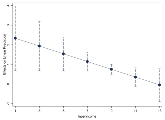
Figure 4.
Difference of the effect of income inequality on hosuehold carbon emissions among households at different per capita income levels: Y-axis is marginal effect coefficient on income inequality, and X-axis is the different levels of household per capita income. The marginal effect coefficients are significant at the 1% level when less than 11, otherwise not significant. The solid line connects the estimation coefficients of income inequality, and the dotted line connects the 95% confidence interval of the estimation coefficients of the key explanatory variable.
As Column (3) of Table 5 shows, the coefficient on the interaction term is negative and significant at the 10% level. We can see clear evidence from the visual results of Figure 5 that a household with an elderly head is less affected by income inequality. This is consistent with our intuition. Elderly people may earn more and have a more peaceful mind; however, the younger ones are easily affected by income inequality, thus spending more on conspicuous consumption to keep up with the Joneses.
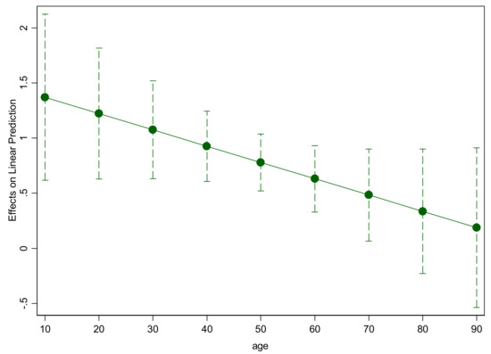
Figure 5.
Difference of the effect of income inequality on hosuehold carbon emissions acmong households with heads of different ages: Y-axis is marginal effect coefficient on income inequality, and X-axis is different ages of the heads of households. The marginal effect coefficients are significant at the 5% level when the heads of households are belows 80, otherwise not significant. The solid line connects the estimation coefficients of income inequality, and the dotted line connects the 95% confidence interval of the estimation coefficients of the key explanatory variable.
5. Conclusions and Policy Implications
In recent years, an increasing number of scholars are paying attention to the relationship between income inequality and climate change. However, there is limited research focusing on the carbon consumption of micro body: households. The current article estimates the effect of income inequality on household carbon emissions in China based on a nationwide CFPS dataset from the period 2010–2014. Lewbel’s (2012) approach is used to deal with the endogenous problem. This paper studies the role of consumption patterns, time preference for consumption and mental health in the relationship. Furthermore, this paper explores the heterogeneity effect of inequality on household carbon emissions among households at different income levels and households with heads of different ages.
The results show that household carbon emissions increase with income inequality. The positive effect of income inequality is greater in households with a younger head. As income increases, the contribution of inequality to household carbon emissions decreases, but the highest class is not even affected. We find that the change in consumption patterns caused by income inequality may be an important reason for this result, and a lower time preference and improved mental health can mitigate the positive effect of income inequality on household carbon emissions.
These results have important implications. Firstly, this paper verifies that income inequality has a positive impact on household carbon emissions in China. Currently, there is a great income gap among citizens, so the government must deepen reforms of the income distribution system and improve the living conditions of low-income households. Secondly, we demonstrate that consumption patterns, time preference for consumption, and mental health can affect the positive impacts of income inequality on household carbon emissions. Reducing income inequality may help improve environmental quality and create a win–win situation, but it cannot be achieved overnight. Therefore, the government can guide consumers to resist consumption competition through the Internet and other media and help consumers to establish an appropriate and green concept of consumption. Furthermore, corresponding policies should be issued to encourage the consumer to invest in the future rather than in current consumption, especially in areas with a high degree of income inequality. A mechanism for social psychological counseling should be established to improve consumers’ mental health, for example, by establishing and subsidizing community counseling centers. Thirdly, concerning the differences in the effect of income inequality on carbon emissions among households at different income levels and households with heads of different ages, it is necessary to adopt different approaches to reduce the carbon emissions of heterogeneous households. For instance, the government should pay more attention to improving the income situation of low-income people, especially the younger low-income people, and to promoting green consumption behaviors in a more acceptable way for young people.
Owing to the limitation of data, we assume that there is the same carbon intensity in 2010, 2012, and 2014 in the empirical analysis. However, in fact, in the global energy conservation environment, the production sector has made a great contribution to emission reduction through decreasing carbon intensity. In the future research, we should take the change of carbon intensity into consideration. Moreover, using energy-saving products is an important way to reduce household carbon emissions, thus, it is worth exploring the effect of income inequality on households’ choice of green home appliances.
Author Contributions
The study conception and design, Y.L. and M.Z.; Data collection and analysis, M.Z. and R.L.; Writing—r original draft, M.Z.; Writing—review & editing, Y.L. and M.Z. All authors have read and agreed to the published version of the manuscript.
Funding
This work was funded by the surface of National Natural Science Foundation of China [grant number 71773011]; the National “Four Batches” Talents of China [grant number 47]; and the Key Project and Social science Research by the ministry of education [grant number13JZD023]; the Research Fund Project of School of Public Affairs, Chongqing University [grant number 2019GGXY001].
Conflicts of Interest
The authors declare no conflicts of interest.
References
- IPCC. Global Warming of 1.5 °C. An IPCC Special Report on the Impacts of Global Warming of 1.5 °C above Pre-Industrial Levels and Related Global Greenhouse Gas Emission Pathways. In The Context of Strengthening the Global Response to the Threat of Climate Change, Sustainable Development, and Efforts to Eradicate Poverty; IPCC: Geneva, Switzerland, 2018; in press. [Google Scholar]
- UNEP (United Nations Environment Program). The Emissions Gap Report 2019; United Nations Environment Programme (UNEP): Nairobi, Kenya, 2019. [Google Scholar]
- World Bank. Growth and CO2 Emissions: How Do Different Countries Fare; Environment Department: Washington, DC, USA, 2007.
- Hao, Y.; Chen, H.; Zhang, Q. Will income inequality affect environmental quality? Analysis based on China’s provincial panel data. Ecol. Indic. 2016, 67, 533–542. [Google Scholar] [CrossRef]
- Guo, D.; Chen, H.; Long, R.; Ni, Y. An integrated measurement of household carbon emissions from a trading-oriented perspective: A case study of urban families in Xuzhou, China. J. Clean. Prod. 2018, 188, 613–624. [Google Scholar] [CrossRef]
- Ji, Q.; Zhang, D. China’s crude oil futures: Introduction and some stylized facts. Financ. Res. Lett. 2019, 28, 376–380. [Google Scholar] [CrossRef]
- Xu, K.; Han, Y.; Lv, F. Household carbon inequality in urban China, its sources and determinants. Ecol. Econ. 2016, 128, 77–86. [Google Scholar] [CrossRef]
- Bin, S.; Dowlatabadi, H. Consumer lifestyle approach to US energy use and the related CO2 emissions. Energy Policy 2005, 33, 197–208. [Google Scholar] [CrossRef]
- Baiocchi, G.; Minx, J.; Hubacek, K. The impact of social factors and consumer behavior on carbon dioxide emissions in the United Kindom. J. Ind. Ecol. 2010, 14, 50–72. [Google Scholar] [CrossRef]
- Pachauri, S.; Spreng, D. Direct and indirect energy requirements of households in India. Energy Policy 2002, 30, 511–523. [Google Scholar] [CrossRef]
- Liu, L.; Wu, G.; Wang, J.; Wei, Y. China’s carbon emissions from urban and rural households during 1992–2007. J. Clean. Prod. 2011, 19, 1754–1762. [Google Scholar] [CrossRef]
- Fan, J.; Liao, H.; Liang, Q.; Tatano, H.; Liu, C.; Wei, Y. Residential carbon emission evolutions in urban-rural divided China: An end-use and behavior analysis. Appl. Energy 2013, 101, 323–332. [Google Scholar] [CrossRef]
- Hertwich, E.G.; Peters, G.P. Carbon footprint of nations: A global, trade-linked analysis. Environ. Sci. Technol. 2009, 43, 6414–6420. [Google Scholar] [CrossRef]
- Wu, S.; Lei, Y.; Li, S. CO2 emissions from household consumption at the provincial level and interprovincial transfer in China. J. Clean. Prod. 2019, 210, 93–104. [Google Scholar] [CrossRef]
- Dong, Y.; Zhao, T. Difference analysis of the relationship between household per capita income, per capita expenditure and per capita CO2 emissions in China: 1997–2014. Atmos. Pollut. Res. 2017, 8, 310–319. [Google Scholar] [CrossRef]
- Stiglitz, J.T. The Price of Inequality: How Today’s Divided Society Endangers Our Future; WW Norton & Company: New York, NY, USA, 2012. [Google Scholar]
- Piketty, T. Capital in the Twenty-First Century; Harvard University Press: Cambridge, MA, USA, 2014. [Google Scholar]
- Ribeiro, W.S.; Bauer, A.; Andrade, M.C.; York-Smith, M.; Pan, P.M.; Pingani, L.; Knapp, M.; Coutinho, E.S.; Evans-Lacko, S. Income inequality and mental illness-related morbidity and resilience: A systematic review and meta-analysis. Lancet Psychiatry 2017, 4, 554–562. [Google Scholar] [CrossRef]
- Burns, J.K.; Tomita, A.; Kapadia, A.S. Income inequality and schizophrenia: Increased schizophrenia incidence in countries with high levels of income inequality. Int. J. Soc. Psychiatry 2014, 60, 185–196. [Google Scholar] [CrossRef]
- Layte, R.; Whelan, C. GINI DP 78: Who Feels Inferior? A Test of the Status Anxiety Hypothesis of Social Inequalities in Health; AIAS, Amsterdam Institute for Advanced Labour Studies: Amsterdam, The Netherlands, 2013. [Google Scholar]
- Vanderende, K.E.; Young, I.K.M.; Dynes, M.M.; Sibley, L.M. Community-level correlates of intimate partner violence against women globally: A systematic review. Soc. Sci. Med. 2012, 75, 1143–1155. [Google Scholar] [CrossRef]
- Kumhof, M.; Rancière, R.; Winant, P. Inequality, Leverage, and Crises. Am. Econ. Rev. 2015, 105, 1217–1245. [Google Scholar] [CrossRef]
- Wolde-Rufael, Y.; Idowu, S. Income distribution and CO2 emission: A comparative analysis for China and India. Renew Sustain Energy Rev. 2017, 4, 1336–1345. [Google Scholar] [CrossRef]
- Solt, F. Standardizing the world income inequality database. Soc. Sci. Q. 2009, 90, 231–242. [Google Scholar] [CrossRef]
- Jorgenson, A.; Schor, J.; Huang, X.R. Income inequality and carbon emissions in the United States: A State-level Analysis, 1997–2012. Ecol. Econ. 2017, 134, 40–48. [Google Scholar] [CrossRef]
- Boyce, J.K. Inequality as a cause of environmental degradation. Ecol. Econ. 1994, 3, 169–178. [Google Scholar] [CrossRef]
- Scruggs, L.A. Political and economic inequality and the environment. Ecol. Econ. 1998, 26, 259–275. [Google Scholar] [CrossRef]
- Heerink, N.; Mulatu, A.; Bulte, E. Income inequality and the environment: Aggregation bias in environmental Kuznets curves. Ecol. Econ. 2001, 3, 359–367. [Google Scholar] [CrossRef]
- Ravallion, M.; Heil, M.; Jalan, J. CO2 emissions and income inequality. Oxf. Econ. Pap. 2000, 4, 651–669. [Google Scholar] [CrossRef]
- Heil, M.; Selden, T. CO2 emissions and economic development: Future trajectories based on historical experience. Environ. Dev. Econ. 2001, 1, 63–83. [Google Scholar] [CrossRef]
- Borghesi, S. Income inequality and the environmental Kuznets curve. In Environment, Inequality Collective Action; Routledge: London, UK, 2006. [Google Scholar]
- Schor, J. The Overspent American: When Buying Becomes You; Basic books: New York, NY, USA, 1998. [Google Scholar]
- Veblen, T. The Theory of the Leisure Class; Oxford University Press: Oxford, UK, 2009. [Google Scholar]
- Golley, J.; Meng, X. Income inequality and carbon dioxide emissions: The case of Chinese urban households. Energy Econ. 2012, 34, 1864–1872. [Google Scholar] [CrossRef]
- Baek, J.; Gweisah, G. Does income inequality harm the environment? Empirical evidence from the United States. Energy Policy 2013, 62, 1434–1437. [Google Scholar] [CrossRef]
- Jorgenson, A. Inequality and the carbon intensity of human well-being. J. Environ. Stud. Sci. 2015, 3, 277–282. [Google Scholar] [CrossRef]
- Kasuga, H.; Takaya, M. Does inequality affect environmental quality? Evidence from major Japanese cities. J. Clean. Prod. 2017, 142, 3689–3701. [Google Scholar] [CrossRef]
- Liu, C.; Jiang, Y.; Xie, R. Does income inequality facilitate carbon emission reduction in the US? J. Clean. Prod. 2019, 217, 380–387. [Google Scholar] [CrossRef]
- Uzar, U.; Eyuboglu, K. The nexus between income inequality and CO2 emissions in Turkey. J. Clean. Prod. 2019, 227, 149–157. [Google Scholar] [CrossRef]
- Coondoo, D.; Dinda, S. Carbon dioxide emission and income: A temporal analysis of cross-country distributional patterns. Ecol. Econ. 2008, 65, 375–385. [Google Scholar] [CrossRef]
- Baloch, A.; Shah, S.Z.; Noor, Z.M.; Magsi, H.B. The nexus between income inequality, economic growth and environmental degradation in Pakistan. Geo J. 2018, 83, 207–222. [Google Scholar] [CrossRef]
- Hübler, M. The inequality-emissions nexus in the context of trade and development: A quantile regression approach. Ecol. Econ. 2017, 134, 174–185. [Google Scholar] [CrossRef]
- Sager, L. Income inequality and carbon consumption: Evidence from environmental Engel curves. Energy Econ. 2019, 84, 104507. [Google Scholar] [CrossRef]
- Grunewald, N.; Klasen, S.; Martínez-Zarzoso, I.; Muris, C. The Trade-off between income inequality and carbon dioxide emissions. Ecol. Econ. 2017, 142, 249–256. [Google Scholar] [CrossRef]
- Clément, M.; Meunié, A. Inégalités, développement et qualité de l’environnement: Mécanismes et application empirique. Mondes En Développement 2010, 151, 67–82. [Google Scholar] [CrossRef]
- Policardo, L. Is democracy good for the environment? Quasi-experimental evidence from regime transitions. Environ. Resour. Econ. 2016, 2, 275–300. [Google Scholar] [CrossRef]
- Waston, B.; Osberg, L. Can positive income anticipations reverse the mental health impacts of negative income anxieties. Econ. Hum. Biol. 2019, 35, 107–122. [Google Scholar]
- Vilhjalmsdottir, A.; Gardarsdottir, R.B.; Bernburg, J.G.; Sigfusdottir, I.D. Neighborhood income inequality, social capital and emotional distress among adolescents: A population-based study. J. Adolesc. 2016, 51, 92–102. [Google Scholar] [CrossRef]
- Layte, R. The association between income inequality and mental health: Testing status anxiety, social capital, and neo-materialist explanations. Eur. Sociol. Rev. 2011, 28, 498–511. [Google Scholar] [CrossRef]
- Chiavegatto Filho, A.D.; Kawachi, I.; Wang, Y.P.; Viana, M.C.; Andrade, L.H. Does income inequality get under the skin? A multilevel analysis of depression, anxiety and mental disorders in Sao Paulo, Brazil. J. Epidemiol. Community Health 2013, 67, 966–972. [Google Scholar] [CrossRef]
- Oishi, S.; Kesebir, S. Income inequality explains shy economic growth does not always translate to an increase in happiness. Psychol. Couns. 2015, 26, 1630–1638. [Google Scholar]
- Velek, C.; Steg, L. Human behavior and environmental sustainability: Problems, driving forces, and research topics. J. Soc. Issues 2007, 63, 1–19. [Google Scholar] [CrossRef]
- Kaida, N.; Kaida, K. Pro-environmental behavior correlates with present and future subjective well-being. Environ. Dev. Sustain. 2016, 18, 111–127. [Google Scholar] [CrossRef]
- Koenig-Lewis, N.; Palmer, A.; Dermody, J.; Urbye, A. Consumers’ evaluations of ecological packaging-rational and emotional approaches. J. Environ. Psychol. 2014, 37, 94–105. [Google Scholar] [CrossRef]
- Bissing-Olson, M.J.; Iyer, A.; Fielding, K.S.; Zacher, H. Relationships between daily affect and pro-environmental behavior at work: The moderating role of pro-environmental attitude. J. Organ. Behav. 2013, 34, 151–171. [Google Scholar] [CrossRef]
- Ibanez, L.; Moureau, N.; Roussel, S. How do incidental emotions impact pro-environmental behavior? Evidence from the dictator game. J. Behav. Exp. Econ. 2017, 66, 150–155. [Google Scholar] [CrossRef]
- Li, J.; Zhang, D.; Su, B. The impact of social awareness and lifestyles on household carbon emissions in China. Ecol. Econ. 2019, 160, 145–155. [Google Scholar] [CrossRef]
- Wei, Y.; Liu, L.; Fan, Y.; Wu, G. The impact of lifestyle on energy use and CO2 emission: An empirical analysis of China’s residents. Energy Policy 2007, 35, 247–257. [Google Scholar] [CrossRef]
- Su, B.; Ang, B.W. Multiplicative decomposition of aggregate carbon intensity change using input-output analysis. Appl. Energy 2015, 154, 13–20. [Google Scholar] [CrossRef]
- Zhang, Q.; Churchill, S.A. Income inequality and subjective wellbeing: Panel data evidence from China. China Econ. Rev. 2020, 60, 101392. [Google Scholar] [CrossRef]
- Zhang, W.; Shi, P.; Wang, K.; Xue, J.; Song, G.; Sun, P. Intertemporal lifestyle changes and carbon emissions: Evidence from a China household survey. Energy Econ. 2020, 86, 104655. [Google Scholar] [CrossRef]
- Liu, Q.; Wang, S.; Zhang, W.; Li, J.; Kong, Y. Examining the effects of income inequality on CO2 emissions: Evidence from non-spatial and spatial perspectives. Appl. Energy 2019, 236, 163–171. [Google Scholar] [CrossRef]
- Andersson, D.; Nässén, J.; Larsson, J.; Holmber, J. Greenhouse gas emissions and subjective well-being: An analysis of Swedish households. Ecol. Econ. 2014, 102, 75–82. [Google Scholar] [CrossRef]
- Streimikiene, D.; Volochovic, A. The impact of household behavioral changes on GHG emission reduction in Lithuania. Renew. Sustain. Energy Rev. 2011, 15, 4118–4124. [Google Scholar] [CrossRef]
- Büchs, M.; Schnepf, S.V. Who emits most? Associations between socio-economic facts and UK households’ home energy, transport, indirect and total CO2 emissions. Ecol. Econ. 2013, 90, 114–123. [Google Scholar] [CrossRef]
- Dai, H.; Masui, T.; Matsuoka, Y.; Fujimori, S. The impacts of China’s household consumption expenditure patterns on energy demand and carbon emissions towards 2050. Energy Policy 2012, 50, 736–750. [Google Scholar] [CrossRef]
- Lee, S.; Lee, B. The influence of urban form on GHG emissions in the US household sector. Energy Policy 2014, 68, 534–549. [Google Scholar] [CrossRef]
- Chancel, L. Are younger generations higher carbon emitters than their elders? Inequalities, generations and CO2 emissions in France and in the USA. Ecol. Econ. 2014, 100, 195–207. [Google Scholar] [CrossRef]
- Jones, C.; Kammen, D.M. Spatial distribution of U.S. Household carbon footprints reveals suburbanization undermines greenhouse gas benefits of urban population density. Environ. Sci. Technol. 2014, 48, 895–902. [Google Scholar] [CrossRef]
- Meier, H.; Rehdanz, K. Determinants of residential space heating expenditures in Great Britain. Energy Econ. 2010, 32, 949–959. [Google Scholar] [CrossRef]
- Ottelin, J.; Heinonen, J.; Junnila, S. Carbon footprint trends of metropolitan residents in Finland: How strong mitigation policies affect different urban zones. J. Clean. Prod. 2018, 170, 1523–1535. [Google Scholar] [CrossRef]
- Qu, J.; Liu, L.; Zeng, J.; Zhang, Z.; Wang, J.; Pei, H.; Dong, L.; Liao, Q.; Maraseni, T. The impact of income on household CO2 emissions in China based on a large sample survey. Sci. Bull. 2019, 64, 351–353. [Google Scholar] [CrossRef]
- Ewing, R.; Rong, F. The impact of urban form on us residential energy use. Hous. Policy Debate 2008, 19, 1–30. [Google Scholar] [CrossRef]
- Qin, B.; Han, S. Planning parameters and household carbon emission: Evidence from high-and low-carbon neighborhoods in Beijing. Habitat Int. 2013, 37, 52–60. [Google Scholar] [CrossRef]
- Lewbel, A. Using heteroscedasticity to identify and estimate mismeasured and endogenous regressor models. J. Bus. Econ. Stat. 2012, 30, 67–80. [Google Scholar] [CrossRef]
- Casaló, L.V.; Escario, J.J. Heterogeneity in the association between environmental attitudes and pro-environmental behavior: A multilevel regression approach. J. Clean. Prod. 2018, 175, 155–163. [Google Scholar] [CrossRef]
- Li, J.; Zhang, J.; Zhang, D.; Ji, Q. Does gender inequality affect household green consumption behavior in China? Energy Policy. 2019, 135, 111071. [Google Scholar] [CrossRef]
- Miao, L. Examining the impact factors of urban residential energy consumption and CO2 emissions in China-Evidence from city-level data. Ecol. Indic. 2017, 73, 29–37. [Google Scholar] [CrossRef]
- Bai, Y.; Deng, X.; Gibson, J.; Zhao, Z.; Hu, H. How does urbanization affect residential CO2 emissions? An analysis on urban agglomerations of China. J. Clean. Prod. 2019, 209, 876–885. [Google Scholar] [CrossRef]
- Topcu, M.; Tugcu, C.T. The impact of renewable energy consumption on income inequality: Evidence from developed countries. Renew. Energy 2020, 151, 1134–1140. [Google Scholar] [CrossRef]
- Kleibergen, G.; Paap, R. Generalized reduced rank tests using the singular value decomposition. J. Econom. 2006, 133, 97–126. [Google Scholar] [CrossRef]
- De Maio, F.G. Income inequality measures. J. Epidemiol. Community Health 2007, 61, 849–852. [Google Scholar] [CrossRef] [PubMed]
- Cobham, A.; Sumner, A.; Cornia, A.; Dercon, S.; Engberg-pedersen, L.; Evans, M.; Lea, N.; Lustig, N.; Manning, R.; Milanovic, B.; et al. Putting the Gini Back in the Bottle? ‘The Palma’ As a Policy-Relevant Measure of Inequality; King’s College WP-5: London, UK, 2013. [Google Scholar]
- Palma, J.G. Homogeneous middles vs. Heterogeneous tails, and the end of the ‘inverted-U’: it’s all about the share of the rich. Dev. Chang. 2011, 42, 87–153. [Google Scholar] [CrossRef]
- Lyons, S.; Pentecost, A.; Tol, R.S.J. Socioeconomic distribution of emissions and resource use in Ireland. J. Environ. Manag. 2012, 112, 186–198. [Google Scholar] [CrossRef] [PubMed]
- Wiedenhofer, D.; Guan, D.; Liu, Z.; Meng, J.; Zhang, N.; Wei, Y.M. Unequal household carbon footprints in China. Nat. Clim. Chang. 2016, 7, 75–80. [Google Scholar] [CrossRef]
- Charles, K.K.; Hurst, E.; Roussanov, N. Conspicuous consumption and race. Q. J. Econ. 2009, 124, 425–467. [Google Scholar] [CrossRef]
- Kaus, W. Conspicuous consumption and “race”: Evidence from South Africa. J. Dev. Econ. 2013, 100, 63–73. [Google Scholar] [CrossRef]
- Zhou, G.; Fan, G.; Ma, G. The impact of income inequality on the visible expenditure of China’s households. Financ. Trade Econ. 2018, 39, 21–35. [Google Scholar]
- Kessler, R.C.; Andrews, G.; Colpe, L.J.; Hiripi, E.; Mroczek, D.K.; Normand, S.L.; Walters, E.E.; Zaslavsky, A.M. Short screening scales to monitor population prevalences and trends in non-specific psychological distress. Psychol. Med. 2002, 6, 959–976. [Google Scholar]
© 2020 by the authors. Licensee MDPI, Basel, Switzerland. This article is an open access article distributed under the terms and conditions of the Creative Commons Attribution (CC BY) license (http://creativecommons.org/licenses/by/4.0/).